Theoretical relationship between stomatal resistance and surface
temperatures in sparse vegetation
J.P. Lhomme
∗,1, B. Monteny
Centre d’Ecologie Fonctionnelle et Evolutive, CNRS, 1919 route de Mende, 34293 Montpellier Cedex 5, France
Received November 1999; received in revised form 5 April 2000; accepted 12 April 2000
Abstract
The relationship between stomatal resistance and foliage temperature in sparse vegetation has been the subject of previous papers [Smith, R.C.G., Barrs, H.D., Fischer, R.A., 1988. Agric. Forest. Meteorol. 42, 183–198; Shuttleworth, W.J., Gurney, R.J., 1990. Q. J. R. Meteorol. Soc. 116, 497–519], in which the modeling is based upon the one-dimensional two-layer approach of Shuttleworth and Wallace [Shuttleworth, W.J., Wallace, J.S., 1985. Q. J. R. Meteorol. Soc. 111, 839–855]. In both studies, however, a major assumption exists concerning the contribution of the substrate to the evaporation process. Using the same approach as these previous studies, an extended and upgraded model is presented in the sense that it relates stomatal resistance to foliage and substrate temperatures (TfandTs) without any assumption on substrate contribution. A comparison of
stomatal resistances estimated from component temperatures (TfandTs) with values measured on fallow savannah during the
HAPEX–Sahel experiment confirms the good performance of the model. Numerical simulations show the general behavior of the relationship between stomatal resistance and foliage temperature in several scenarios involving various weather conditions and canopy characteristics. The sensitivity of the calculated stomatal resistance to input variables and model parameters is investigated. It is shown that the calculation of stomatal resistance exhibits a significant sensitivity to foliage temperature and a much lesser one to substrate temperature. Uncertainties in leaf area index have a relatively weak impact on the calculated stomatal resistance. The sensitivity of stomatal resistance to the two main coefficients involved in the partitioning of available energy has also been investigated. © 2000 Elsevier Science B.V. All rights reserved.
Keywords:Sparse vegetation; Stomatal resistance; Two-layer model; Radiometric surface temperature; Foliage and substrate temperature
1. Introduction
In the assessment of vegetation water status the measurement of foliage temperature by infrared thermometry can be very helpful as a stress indicator. Its use stems from the fact that when the stomatal closure resulting from a water stress occurs, the
tran-∗Corresponding author. Fax:+33-4-67-4121-38.
E-mail address:[email protected] (J.P. Lhomme)
1Permanent address: IRD (previously ORSTOM), 213 rue La
Fayette, 75010 Paris, France.
spiration rate reduces and foliage temperature rises due to a decrease in energy dissipation. The idea of using plant foliage temperatures as a stress indicator has been popularized in the early 1980s by Idso and Jackson (Idso et al., 1981; Jackson et al., 1981) in the form of the crop water stress index (CWSI). This index, based upon the difference between the actual canopy temperature and that of an unstressed base-line, has led to important agricultural applications such as irrigation scheduling and crop yield predic-tion. When vegetation is sparse and when temperature measurements are made from hand-held, airborne or
satellite-based infrared sensors, foliage temperature is often difficult to separate from the soil component, which makes the CWSI poorly reliable. To overcome this difficulty, Moran et al. (1994) developed the veg-etation index-temperature (VIT) trapezoid method, based on a combination of spectral vegetation indices and composite surface temperature measurements. Jones (1999) modified the calculation of the CWSI by replacing theoretical estimates of the upper bound and baseline temperatures by measured temperatures of appropriate reference surfaces.
Concurrently, attempts have been made to
directly determine canopy resistance from the surface temperature of the foliage, as measured by infrared thermometry, in conjunction with standard meteoro-logical measurements above the canopy. When there is complete canopy cover, the single-layer approach underlying the Penman–Monteith equation (Monteith, 1965) provides an adequate basis for this determina-tion (Jackson et al., 1981; Hatfield, 1985). For sparse vegetation, the problem is not so straightforward. Smith et al. (1988) developed and tested a two-layer approach based on the Shuttleworth–Wallace model (1985) to calculate the mean stomatal resistance of a sparse crop from infrared measurements of foliage temperature. However, a major drawback of their approach is that the theoretical expression of foliage resistance is a function of soil evaporation that is a pri-ori unknown. Their assumption of using equilibrium evaporation as an estimate of soil evaporation limits the applicability of their method because evidently it does not hold when soil dries out. In a similar man-ner, Shuttleworth and Gurney (1990) investigated the performance of the Shuttleworth–Wallace model to calculate the canopy resistance from measurements of foliage temperature. But the exacting assumption ap-pearing in Smith et al. (1988) still exists in the form of a fixed and arbitrary value of soil surface resistance. They recognize (quote) that: “In practical applica-tions a better specification of substrate interaction is identified as the primary problem in using this theory in very sparse canopies”, adding that “a measurement of substrate temperature used in conjunction with [basic equations] represents an attractive and simple alternative” (Shuttleworth and Gurney, 1990, p. 517). The present study follows the lines drawn by these previous papers in the sense that it aims at present-ing and evaluatpresent-ing the theoretical basis needed to infer
stomatal resistance in sparse vegetation from measure-ments of radiometric surface temperature. It is shown that stomatal resistance can be calculated in a more re-liable manner than in the previous models, i.e. without major assumption concerning the substrate interaction, when foliage and substrate temperatures are simul-taneously used in the calculation. Consequently, the model presented constitutes an upgrading of the pre-vious models of Smith et al. (1988) and Shuttleworth and Gurney (1990). The paper is divided into two main sections. The first section infers the theoretical expres-sion relating stomatal resistance to foliage and sub-strate temperatures. The second section presents the practical implementation of the model with an experi-mental validation, numerical simulations and a sensi-tivity analysis.
2. Theoretical development
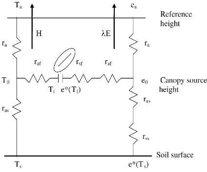
The basic equations used are those of the one-dimensional two-layer model originally devised by Shuttleworth and Wallace (1985) and updated by Choudhury and Monteith (1988) and Shuttleworth and Gurney (1990) (Fig. 1). This model is based on
diffusion theory (K-theory) even though turbulent
transport within canopies is not a strict diffusive pro-cess. In the recent years, news theories have been
developed to describe the turbulent transport of scalar within the canopy such as the ‘higher-order-closure’ approach (Meyers and Paw U, 1987) or the La-grangian approach (Raupach, 1989). Unfortunately, these new approaches, which are supposed to replace
the traditional K-theory, are generally too complex
to be easily implemented in simple canopy models for practical applications. In the Lagrangian approach the profile of scalar concentration is described as the sum of a far-field contribution predicted by diffu-sion theory and a near-field contribution, for which the diffusion equation fails. Van den Hurk and Mc-Naughton (1995) showed that the non-diffusive part of the transport process in a two-layer resistance model could be accounted for by adding a near-field resistance in series with the bulk boundary-layer resistance of the upper-layer (foliage). Although sur-prising, this additional resistance has been found to be small in comparison with other aerodynamic resis-tances (with a small effect on canopy microclimate) and does not call into question the basic principles of the Shuttleworth–Wallace model. McNaughton and van den Hurk (1995) completed the revision of the two-layer model by evaluating the other
re-sistances. Their conclusion is (quote) “K-theory (in
the guise of far-field theory) is an adequate basis for constructing two-layer models”, which justifies the approach used in the following development.
2.1. Formulation of stomatal resistance
Energy balance equations for the vegetation layer and the substrate layer can be detailed respectively
as a function of foliage temperatureTf and substrate
temperatureTsin the following manner (Shuttleworth
and Wallace, 1985; Choudhury and Monteith, 1988)
A−As=
whereA=Rn−Gis the total available energy, withRn
the net radiation andGthe soil heat flux;As=Rns−G
the available energy of the substrate level, withRns
the net radiation reaching the substrate. T0 and e0
are the air temperature and the air vapour pressure at canopy source height, respectively.e∗(T) denotes the saturated vapor pressure at temperatureT.ras denotes
the aerodynamic resistance between the substrate and
the canopy source height andraf is the bulk
bound-ary layer resistance of the canopy foliage.rss is the
substrate resistance, rsf the foliage resistance to
wa-ter vapor transfer,γ the psychrometric constant,ρthe
air density andcp is the specific heat of air at
con-stant pressure. These basic equations can be solved for substrate and foliage resistances by means of the following manipulations. Linearizing the difference of saturated pressure between the foliage and the canopy source height leads to
e∗(Tf)−e0=D0+s(Tf−T0) (3)
whereD0is the water vapor pressure deficit at canopy
source height and sthe slope of the saturated vapor
pressure curve at the temperature of the air. The
sen-sible heat fluxHwritten between the canopy source
height and the reference height gives
T0=Ta+Hra
ρcp
(4)
A similar equation can be written for the saturation deficit (Shuttleworth and Wallace, 1985, Eq. (8))
D0=Da+
[H (s+γ )−γ A]ra
ρcp
(5)
Combining Eqs. (3)–(5) with Eq. (1) leads to
rsf =(Da/γ )−[Ara+(A−As)raf]/ρcp+(1+s/γ )(Tf−Ts)
(A−As)/ρcp+[Hra/(ρcp)−(Tf−Ta)]/raf
(6)
Writing that the total flux of sensible heat is the sum of the contributions from each layer
H=ρcp[(Tf−T0)/raf+(Ts−T0)/ras] and taking into
account Eq. (4) leads to
H= ρcp[(Ts/ras+Tf/raf)−Ta(1/ras+1/raf)]
[1+ra(1/ras+1/raf)]
(7)
ReplacingHin Eq. (6) by Eq. (7) yields the following
rsf =
(Da/γ )−[Ara+(A−As)raf]/ρcp+(1+s/γ )(Tf−Ta)
(A−As)/ρcp+(ra(Ts−Tf)+ras(Ta−Tf))/(ra(raf+ras)+rasraf)
(8)
The mean stomatal resistancerst (per unit leaf area)
is calculated as rst=rsfL0, where L0 is the leaf area
index (Lhomme, 1991). We have to note that a similar calculation carried out on the basis of substrate energy balance (2) leads to a similar expression for substrate resistance
rss=
(Da/γ )−(Ara+Asras)/ρcp+(1+s/γ )(Ts−Ta)
(As/ρcp)+(ra(Tf−Ts)+raf(Ta−Ts))/(ra(ras+raf)+rafras)
(9)
Eq. (8) should be valid for the limit case of a closed canopy. When there is no substrate interaction,
As=0 and the resistance ras is infinite in Eq. (8),
which means that the expression of rsf transforms
into
rsf=
(Da/γ )−A(ra+raf)/ρcp+(1+s/γ )(Tf−Ta)
(A/ρcp)+(Ta−Tf)/(ra+raf)
(10)
This equation is directly obtained from the one-layer description of the vegetation–atmosphere interac-tion following the simpler Penman–Monteith format (Shuttleworth and Gurney, 1990, Eq. (4)).
2.2. Specification of air resistances and available energy partition
The aerodynamic resistancera (assumed to be the
same for heat and water vapor) is calculated by means of the classical formula that takes into account the stability correction functions for wind and temperature (Brutsaert, 1982)
the integral diabatic correction functions respec-tively for heat and momentum given by Paulson
(1970). L is the Monin–Obukhov length defined by
L=−ρcpTau3∗/(kgH), whereu∗is the friction velocity, gis the acceleration of gravity,Ta is the air
tempera-ture expressed in Kelvin andHis the sensible heat flux
counted positively upwards. The zero plane
displace-ment heightdand the roughness length for momentum
z0are determined following Choudhury and Monteith
(1988), who fitted simple functions to the curves ob-tained by Shaw and Pereira (1982) from second-order
closure theory
wherecd=0.2 is the mean drag coefficient assumed
to be uniform within the canopy,h is the height of
the canopy andz0sis the roughness length of the
sub-strate. For bare soilz0s is commonly taken as 0.01 m
(Shuttleworth and Wallace, 1985). For vegetated
sub-strate, z0s is calculated as one-tenth of the height
of the lower vegetation (Lhomme et al., 1997). The formulations of the resistances within the canopy
are essentially those based onK-theory proposed by
Choudhury and Monteith (1988). The aerodynamic resistance between the substrate and the source height of the whole canopy (d+z0) is defined as the integral
of the reciprocal of eddy diffusivity over the height range [z0s,d+z0]
K(h) is the value of eddy diffusivity at canopy height given by
raf=
αw[w/u(h)]1/2
4α0L01−exp(−αw/2)
(16)
w is the leaf width,α0andαw are constants
respec-tively equal to 0.005 m s−1/2and 2.5 (dimensionless),
u(h) is the wind speed at canopy height calculated as
u(h)=ua{ln[(h−d)/z0]−9m(h/L)}
{ln[(zr−d)/z0]−9m(zr/L)}
(17)
The net radiation reaching the soil surface Rns is
calculated using a Beer’s law of the form
Rns=Rn exp(−αrL0) (18)
where αr is the extinction coefficient. Shuttleworth
and Wallace (1985) and Shuttleworth and Gurney
(1990) arbitrarily prescribed a value of 0.7 for αr in
sparse crops, whereas Kustas and Norman (1997) as-signed a value of 0.45, considered as (quote) “midway between its likely limits of 0.3–0.6”. A compromise has been retained in our study by fixing an arbitrary value of 0.5 following Choudhury (1989). This value is used both in the experimental validation and the numerical simulations. When not available by direct
measurement, the soil heat flux Gcan be calculated
as a given fraction αg (≈0.3) of the net radiation
reaching the substrate:G=αgRns.
2.3. Determination of component temperatures
Component temperatures Tf and Ts can be
di-rectly measured using an IRT sensor with a narrow acceptance angle to avoid the contamination of fo-liage temperature by substrate temperature. They can also be determined by calculation from directional measurements of canopy surface temperature (i.e. made at two different angles). A brief outline is given hereafter. In a two-layer representation of the whole
canopy the radiometric surface temperatureTr is
ex-pressed as a function of the component temperatures as (Norman et al., 1995)
Tr=
h
f (ϕ)Tf4+(1−f (ϕ))Ts4i1/4 (19)
wheref(ϕ) is the fraction of the field of view of the radiometer occupied by vegetation (a function of the
view zenith angleϕ) and where the temperatures are
expressed in Kelvin. If one assumes foliage elements to be randomly distributed above the soil surface, the
fractional vegetation area viewed by a radiometer from a zenith angleϕis
whereL0is the leaf area index andαa is a coefficient
which depends upon the angular distribution of foliage elements (Choudhury, 1989). For uniform leaf-angle
distributionαa is equal to 0.5. By assuming that the
difference between the two component temperatures
TfandTs(expressed in Kelvin) is relatively small, the
radiometric surface temperature given by (19) can be approximated by the area-weighted mean of foliage and substrate temperatures (Choudhury, 1989; Nor-man et al., 1995)
Tr=f (ϕ)Tf+[1−f (ϕ)]Ts (21)
If two radiometric surface temperatures Tr1 and Tr2
are measured with two different angles of view ϕ1
and ϕ2, Tf and Ts can be retrieved by solving
al-gebraically either the set of two equations with two unknowns (19) (Kustas and Norman, 1997, Eqs. (7) and (8)) or, with a lesser accuracy, their linearized forms (21)). The problem of retrieving substrate and foliage temperatures from two directional measure-ments of surface temperature has been analyzed with more details by François et al. (1997).
3. Model predictions
3.1. Comparison of model outputs with experimental data
The data used to test the model are taken from the HAPEX–Sahel experiment which took place in Niger in 1992 (Goutorbe et al., 1994). The micrometeo-rological data needed to implement the model were measured on a fallow savannah of the east–central supersite (EC) near the village of Banizoumbou (13◦31′N, 2◦39′E, alt: 240 m). Fallow savannah is a composite vegetation made up of woody shrubs of
Guiera senegalensisscattered above a sparse herba-ceous substrate. The characteristics of the vegetation and the details of the instrumentation have already been described in Lhomme et al. (1994) and Monteny
characteristics: canopy height h=3.5 m, leaf area in-dexL0=0.5, leaf widthw=0.02 m. Bush and substrate
temperatures were measured by two nadir-looking infra-red thermometers (Everest Interscience IRTs), one mounted at 9 m over the grass area (in fact a mix-ture of bare soil and senesced foliage) and the other
at about 1 m above aGuierashrub. Wind velocity, air
temperature and water vapour pressure were measured at a reference height of 12 m above the soil surface. The net radiometer (REBS, Q6, Campbell, UK) was also installed at a height of 12 m. Soil heat flux was measured by flux plates buried at a depth of 3 cm. All the micrometeorological measurements were logged as 20 min average values on a data acquisition sys-tem. Stomatal resistance was not measured on this site. However, measurements of stomatal resistance were available on a nearby fallow savannah of the west–central supersite (WC) centred on the village of Fandou Beri, 10 km West of Banizoumbou and at the same altitude (Hanan and Prince, 1997). These data are used to test the outputs of the model. Resistance measurements of the lower (abaxial) surface of the leaf were made with a transient porometer (Mark
II, Delta-T Devices, Cambridge, UK) on 12 Guiera
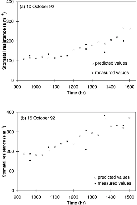
shrubs selected at random on a line transect across the site and point resistance measurements were averaged into hour mean values representing an estimate of the bulk average stomatal resistance of the canopy. More details on the acquisition of stomatal resistance data are given in Hanan and Prince (1997, p. 539). The structural characteristics of the two fallow savannah sites were roughly similar with shrub density a little lower on the WC site (LAI of 0.32 instead of 0.5). Soil characteristics are also very comparable (D’Herbès and Valentin, 1997). Consequently stomatal resistance values should be very similar for a same day on the two sites and the comparison between the outputs of the model obtained at the EC supersite and the mea-surements made at the WC supersite appears to be fully jusifiable. The data of 2 days of October 1992 (10 and 15) were used. They are the only days when simultaneous measurements were made on both sites. The month of October corresponds to the start of the dry season (the last rainfall on the site occured on 14 September). The herbaceous canopy is already nearly dry with a mean height of about 0.5 m. Only the data corresponding to the midday hours, from 9:00 to 15:00 hours, with net radiation generally higher
Fig. 2. For 2 days of October 1992 (10 and 15), diurnal course of stomatal resistance ofGuiera senegalensisbetween 9:00 and 15:00 hours, as predicted by the model on a 20 min basis and as measured by a porometer on an hourly basis (data taken from Hanan and Prince (1997)).
than 400 W m−2, were selected for these 2 days. The
results are shown in Figs. 2 and 3 for the 2 days retained in the comparison. Fig. 2a and b shows the diurnal course of stomatal resistance as calculated by the model (Eq. (8)) from the component temperatures (Ts,Tf) and the micrometeorological data (Rn,G,Ta,
Da,ua) recorded on the EC site and as measured the
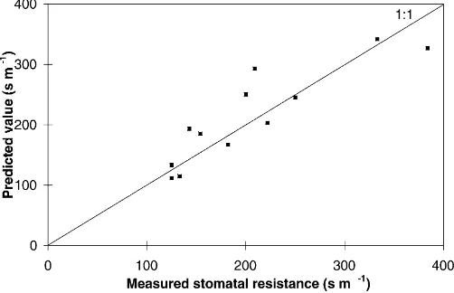
Fig. 3. Predicted values of stomatal resistance vs. measured values on an hourly basis for the 2 days retained in the comparison (10 and 15 October 1992).
between experimental and modeled values is fairly good. Stomatal resistances are higher on 15 October than on 10 October certainly due to an increasing soil water deficit, as no rain has occurred between these two dates; and the diurnal trend exhibits a typical in-crease of stomatal resistance during the diurnal part of the day. Additionally, Fig. 3 shows a plot of predicted versus measured hourly values of stomatal resistance. The scatter is clearly about the 1:1 line, which indi-cates acceptable agreement. Consequently, two main statements can be made from the comparison. Firstly, the values predicted by the model globally coincide with the values measured during these two contrasted days. Secondly, the model accounts well for the char-acteristic rise of stomatal resistance during the central hours of the day.
3.2. Operational expression of stomatal resistance and numerical simulations
The rest of the paper aims at developing an op-erational expression of stomatal resistance in terms
of component temperatures Tf andTs to examine its
general behavior and to assess its sensibility. Net ra-diation and soil heat flux measurements are easy to make and can be directly used as input to the model as shown in the previous section. However, when
avail-able energy is not measured, Rn and G can be
pa-rameterized in terms of standard meteorological data
and canopy characteristics as described below. Rn is
expressed as a function of long-wave radiation
bud-getRl and incoming solar radiationS(a
meteorolog-ical variable commonly measured) in the following way:
Rn=(1−ae)S+Rl Rl=ε(L↓ −σ Tr04) (22)
where ae is the effective surface albedo, ε the
sur-face emissivity assumed to be constant during the
day, σ the Stefan–Boltzmann constant and Tr0 the
nadir radiometric surface temperature. Surface tem-perature being necessarily an input to the model,
Tr0 can be either directly measured or calculated
from component temperatures Tf and Ts by means
of Eq. (19) or (21) with ϕ=0. L↓ is the
incom-ing long-wave radiation which can be calculated by means of the following empirical formula (Brutsaert, 1982)
L↓=εaσ Ta4 εa=0.552e1/7a (23)
whereTa is the air temperature in Kelvin andea the
air vapor pressure expressed in hPa. It is possible to use other formulae for the apparent emissivity of the
atmosphereεa without altering the generality of the
results obtained. The long-wave radiation balance can be rewritten as
Rl=εσ[εaTa4−f0Tf4−(1−f0)Ts4] (24)
where f0=1−exp(−αaL0) is the shielding factor in
area of the substrate covered by the vegetation). It is
obtained from Eq. (20) with ϕ=0. Denoting foliage
and substrate albedos respectively by af andas, the
effective albedo of the two-layer interface is
ae =f0af+(1−f0)2as
This formula is obtained by adding the multiple reflec-tions between the substrate and the canopy (Taconet et al., 1986). Taking into account the formulae derived above, the stomatal resistance formulation (Eq. (8)) transforms into
involves two types of input data: driving variables and canopy characteristics. The driving variables are the standard weather data (air temperature (Ta), air
humid-ity (Daandea), wind velocity (ua), solar radiation (S))
and the component temperatures (Tf andTs) obtained
by infrared thermometry. The canopy is characterized by structural data (canopy height (h), LAI (L0), leaf width (w), roughness length of the substrate (z0s)),
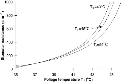
radiative data (component albedos (afandas), surface emissivity (ε)) and pseudo-constant coefficients (cd, α0,αa,αg,αr,αw) related to the type of canopy. Nu-merical simulations have been performed with Eq. (26) using the values of the parameters given in Table 1. Fig. 4 shows the relationship between stomatal resis-tance and foliage temperature for different substrate temperatures in a given scenario with high solar
ra-diation and high air temperature. As expected rst is
Table 1
Standard values of model parameters used in the numerical sim-ulations
aThe values are measured in meters.
an increasing function of Tf. When substrate
temperature increases with foliage temperature kept constant, stomatal resistance decreases. This is due to the fact that the sensible heat flux emanating from the substrate contributes to increasing foliage tempera-ture as stomatal closure does. Since this contribution increases with substrate temperature, the relative con-tribution of stomatal closure to the heating of the foliage at a given foliage temperature is lower for a
higher substrate temperature, which means that rst
Fig. 4. Stomatal resistance vs. foliage temperature for differ-ent substrate temperatures in a given scenario:h=0.5 m, LAI=1, S=1000 W m−2,T
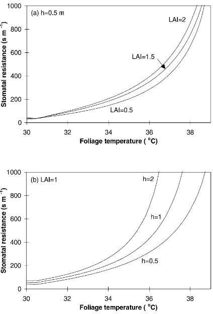
Fig. 5. Stomatal resistance vs. foliage temperature: (a) for different values of LAI; (b) for different values of vegetation heighth(m). S=800 W m−2,T
a=30◦C, RHa=60%,ua=2 m s−1andTs=40◦C.
should be lower. The influence of the main structural characteristics of the canopy (LAI and vegetation
height) on the relation rst=f(Tf) is examined in
Fig. 5a and b. All other conditions being equal, the stomatal resistance increases with an increased LAI for a given foliage temperature. The same behavior occurs with canopy height: The higher the canopy, the greater the stomatal resistance. Fig. 6 illustrates the role of wind velocity. All other conditions being equal, the greater the wind velocity, the greater the stomatal resistance. This result is logical since greater wind velocity leads to increased energy dissipation by convection, which tends to lower the foliage tem-perature. Hence, at a given foliage temperature, stom-atal resistance should be greater for a greater wind velocity.
Fig. 6. Stomatal resistance vs. foliage temperature for different values (1, 2, 4) of wind velocityua(m s−1). The scenario simulated
is: h=0.5 m, LAI=1, S=800 W m−2, T
a=30◦C, RHa=60% and
Ts=40◦C.
3.3. Sensitivity analysis
In the calculation of stomatal resistance from Eq. (26) the major cause of uncertainty certainly
comes from the component temperaturesTf andTs,
either directly measured or estimated from two direc-tional measurements of radiometric surface tempera-ture. We have calculated the relative error made inrst
due to an error in foliage temperatureTfand substrate
temperatureTs, all other quantities being assumed to
be correctly measured or estimated. Differentiating Eq. (26) leads toδrst/rst=δN/N−δD/D,where N and
Dare respectively the numerator and denominator of
Eq. (26). CalculatingδNandδDas a function ofδTf
where the derivatives ofNandD with respect to Tf
andTsare detailed in Appendix A. In a given scenario, the variations ofδrst/rstcorresponding to a given error inTf andTs (δTf=±1◦C andδTs=±1◦C) have been
calculated as a function of foliage temperatureTf. One
Fig. 7. Relative error in stomatal resistance estimate vs. foliage temperature for the range of foliage temperature corresponding ap-proximately to 50<rst<500 s m−1: (a) for a fixed error (|dTf|=1)
in foliage temperature Tf; (b) for a fixed error (|dTs|=1) in
substrate temperature Ts. The scenario simulated is
character-ized by:h=0.5 m, LAI=1,S=800 W m−2,T
a=30◦C, RHa=60%,
ua=2 m s−1.
than 1◦C in practice (mainly because of some
uncer-tainty in the fractional cover estimate). The results of the calculation are shown in Fig. 7. It appears thatrstis very sensitive to an error in foliage temperature since an error of±1◦C leads to a relative error in stomatal resistance of not less than 30%. Conversely,rstis very little sensitive to an error in substrate temperature. An
error of ±1◦C in Ts leads to a relative error much
lower than 5% in stomatal resistance. This means that foliage temperature should be measured or determined with a greater care than substrate temperature because its impact on stomatal resistance estimate is greater. Among the canopy characteristics required as inputs to the model, leaf area index is certainly the most difficult to determine accurately, especially if evaluated with remote sensing techniques (Sellers and Hall, 1993). It is the reason why the model sensitivity to an uncer-tainty in LAI has been studied in the way illustrated in Fig. 8. The relative error (δrst/rst) in stomatal
resis-tance resulting from a±25% variation in LAI is
plot-ted against foliage temperature for a given scenario.
The effect on rst appears to be relatively small: the
relative error is much lower than 5% over the largest part of the temperature range. The sensitivity of stom-atal resistance expression to the main coefficients in-volved in its formulation has also been assessed. Only the two coefficients related to the partitioning of
avail-Fig. 8. Relative error in stomatal resistance estimate resulting from a given error (±25%) in LAI for the same scenario as in Fig. 7 and for the range of foliage temperature corresponding roughly to 50<rst<500 s m−1.
able energy have been retained, namelyαr, which
de-scribes the exponential decay in net radiation within
the canopy, and αg, which determines the soil heat
flux from the net radiation reaching the substrate. The results are shown in Figs. 9 and 10. The magnitude of the response to changes in the other coefficients (those involved in the resistances of the air:cd,α0,αw) has been thoroughly examined by Shuttleworth and Wal-lace (1990) in relation with their proper formulation of stomatal resistance and will not be re-examined here. In sparse and clumped vegetation, the use of Beer’s law (Eq. (18)) for estimating net radiation divergence
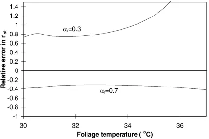
Fig. 9. Relative error in stomatal resistance estimate due to a given error (±0.2) in coefficientαr(involved in the partitioning of
available energy) with the preferred valueαr=0.5. Same scenario
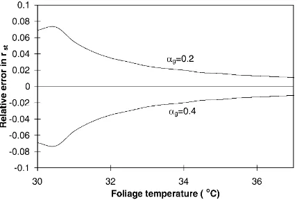
Fig. 10. Relative error in stomatal resistance estimate due to a given error (±0.1) in coefficient αg (involved in soil heat flux
estimation) with the preferred valueαg=0.3. Same scenario and
same conditions as in Fig. 7.
is certainly questionable unless the extinction
coeffi-cientαris properly adjusted. The problem is that the
magnitude of this coefficient is not easily estimated a priori. In Fig. 9, for a given scenario, the relative error made in stomatal resistance (δrst/rst) is plotted versus
foliage temperature when αr is set to its prescribed
value±0.2 (a realistic uncertainty in the case of sparse vegetation). In Fig. 10, the same type of graph is drawn
with αg (Eq. (27)) set to its prescribed value ±0.1
(also a realistic uncertainty). The sensitivity of rst to
αrappears to be much greater than toαg. For the
spe-cific range 30◦C<T
f<37◦C, a variation of +0.2 and
–0.2 in the prescribed value ofαr(0.5) leads to a
rel-ative error a little bit less than−40% and greater than
+70% respectively. On the other hand, a variation of
±0.1 in the prescribed value ofαg(0.3) does not lead
to a relative error greater than 8% (it is lower than 5% on most of the range). Consequently, an accurate
determination of Beer’s law coefficientαr appears to
be determinant in the implementation of this stomatal
resistance model, whereas the role ofαgis of minor
importance.
4. Conclusion
This study has shown how stomatal resistance in sparse vegetation can be inferred from two directional measurements (at two different angles) of the radio-metric surface temperature, without any assumption
concerning the evaporation from the substrate. These two measurements allow one to determine foliage and substrate temperatures; and when these two tem-peratures are known, stomatal resistance is perfectly defined by Eq. (8), at least in theory. For this rea-son, the model presented upgrades and supersedes the previous approaches of Smith et al. (1988) and Shuttleworth and Gurney (1990), both based on the same basic equations but with a similar and signif-icant assumption concerning the contribution of the substrate to the evaporation process. An experimental validation carried out with data collected on fallow sa-vannah during the HAPEX–Sahel experiment shows an adequate agreement between model estimates and measured values. Stomatal resistance, as calculated from the operational expression (26), is very sensitive to an error in foliage temperature, but much less to an error in substrate temperature. This means that fo-liage temperature should be determined with a greater care than substrate temperature. An error in LAI has a relatively minor effect. As to the main coefficients involved in the partitioning of available energy, the coefficient of Beer’s law (αr) has a much greater
influ-ence on the estimation of stomatal resistance than the coefficient relatingGtoRn(αg) and should be chosen with great care. In the future, a possible improvement of the present theory could consist in replacing the simple Beer’s law with a more appropriate radiation model separating short-wave and long-wave radiation balance.
5. Nomenclature
ae canopy effective albedo
A =Rn−G, total available energy (W m−2)
As substrate available energy (W m−2)
cp specific heat of air at constant pressure
(J kg−1K−1)
d zero plane displacement height (m)
Da vapor pressure deficit at reference height
(e∗(Ta)−ea) (Pa)
D0 vapor pressure deficit at canopy source
height (Pa)
ea vapor pressure at reference height (Pa)
e∗(T) saturated vapor pressure at temperature
f(ϕ) fractional vegetation area viewed by the radiometer
f0 =f(0)
G soil heat flux (W m−2)
h canopy height (m)
H total sensible heat flux (W m−2)
k von Karman’s constant (0.4)
K eddy diffusion coefficient (m2s−1)
L Monin–Obukhov’s length (m)
L0 LAI: leaf area index (m2m−2)
ra aerodynamic resistance between the
source height and the reference height (s m−1)
raf bulk boundary layer resistance of the
vegetative elements (s m−1)
ras aerodynamic resistance between the
substrate and the source height (s m−1)
rsf foliage resistance to water vapor
transfer (s m−1)
rst mean stomatal resistance (s m−1)
rss substrate resistance to evaporation (s m−1)
RHa relative humidity at reference height (%)
Rn net radiation of the complete
canopy (W m−2)
Rns net radiation of the substrate (W m−2)
s slope of the saturated vapor pressure curve
atTa(Pa K−1)
S incoming solar radiation (W m−2)
Ta air temperature at reference height (◦C)
Tf foliage temperature (◦C)
Tr radiometric surface temperature (◦C)
Ts substrate (or soil surface) temperature (◦C)
T0 air temperature at canopy source
height=aerodynamic surface temperature
(◦C)
ua wind velocity at reference height (m s−1)
u∗ friction velocity (m s−1)
z0 canopy roughness length for momentum
(m)
z0s roughness length of the substrate (m)
zr reference height (m)
Greek symbols
γ psychrometric constant (Pa K−1)
ϕ view angle of the radiometer to the vertical (◦)
λE total latent heat flux (W m−2)
ρ air density (kg m−3)
Appendix A. Detailed expression of Eq. (31)
As a first approximation the aerodynamic resis-tancesra,rasandrafare assumed to be independent of
component temperaturesTs andTf. This assumption
leads to
Brutsaert, W., 1982. Evaporation into the Atmosphere. Reidel, Dordrecht, 299 pp.
Choudhury, B.J., 1989. Estimating evaporation and carbon assimilation using infrared temperature data: vistas in modeling. In: Asrar, G. (Ed.), Theory and Applications of Optical Remote Sensing. Wiley, New York, pp. 628–690.
Choudhury, B.J., Monteith, J.L., 1988. A four-layer model for the heat budget of homogeneous land surfaces. Q. J. R. Meteorol. Soc. 114, 373–398.
Deardorff, J.W., 1978. Efficient prediction of ground surface temperature and moisture with inclusion of a layer of vegetation. J. Geophys. Res. 83, 1889–1903.
D’Herbès, J.M., Valentin, C., 1997. Land surface conditions of the Niamey region: ecological and hydrological implications. J. Hydrol. 188–189, 18–42
François, C., Ottlé, C., Prévot, L., 1997. Analytical parameteri-zation of canopy directional emissivity and directional radiance in the thermal infrared. Application on the retrieval of soil and foliage temperatures using two directional measurements. Int. J. Remote Sensing 18, 2587–2621.
Goutorbe, J.P., Lebel, T., Tinga, A., Bessemoulin, P., Brouwer, J., Dolman, A.J., Engman, E.T., Gash, J.H.C., Hoepffner, M., Kabat, P., Kerr, Y.H., Monteny, B., Prince, S., Said, F., Sellers, P., Wallace, J.S., 1994. HAPEX–Sahel: a large scale study of land–atmosphere interactions in the semi-arid tropics. Ann. Geophys. 12, 53–64.
Hanan, N.P., Prince, S.D., 1997. Stomatal conductance of west– central supersite vegetation in HAPEX–Sahel: measurements and empirical models. J. Hydrol. 188-189, 536–562. Hatfield, J.L., 1985. Wheat canopy resistance determined by energy
Idso, S.B., Jackson, R.D., Pinter, P.J., Reginato, R.J., Hatfield, J.L., 1981. Normalizing the stress-degree-day parameter for environmental variability. Agric. Meteorol. 24, 45–55. Jackson, R.D., Idso, S.B., Reginato, R.J., Pinter, P.J., 1981. Canopy
temperature as a crop stress indicator. Water Resour. Res. 17, 1133–1138.
Jones, H.G., 1999. Use of infrared thermometry for estimation of stomatal conductance as a possible aid to irrigation scheduling. Agric. For. Meteorol. 95, 139–149.
Kustas, W.P., Norman, J.M., 1997. A two-source approach for estimating turbulent fluxes using multiple angle thermal infrared observations. Water Resour. Res. 33, 1495–1508.
Lhomme, J.P., 1991. The concept of canopy resistance: historical survey and comparison of different approaches. Agric. For. Meteorol. 54, 227–240.
Lhomme, J.P., Monteny, B., Chehbouni, A., Troufleau, D., 1994. Determination of sensible heat flux over Sahelian fallow savannah using infra-red thermometry. Agric. For. Meteorol. 68, 93–105.
McNaughton, K.G., van den Hurk, B.J.J.M., 1995. A ‘Lagrangian’ revision of the resistors in the two-layer model for calculating the energy budget of a plant canopy. Boundary Layer Meteorol. 74, 261–288.
Meyers, T.P., Paw U, K.T., 1987. Modelling the plant canopy micrometeorology with higher-order-closure principles. Agric. For. Meteorol. 41, 143–163.
Monteith, J.L., 1965. Evaporation and environment. Proc. Symp. Soc. Exp. Biol. 19, 205–234.
Monteny, B.A., Lhomme, J.P., Chehbouni, A., Troufleau, D., Amadou, M., Sicot, M., Verhoef, A., Galle, S., Said, F., Lloyd, C.R., 1997. The role of the Sahelian biosphere on the water and the CO2 cycle during the HAPEX–Sahel experiment. J.
Hydrol. 188–189, 516–535.
Moran, M.S., Clarke, T.R., Inoue, Y., Vidal, A., 1994. Estimating crop water deficit using the relation between surface–air
temperature and spectral vegetation index. Remote Sensing Environ. 49, 246–263.
Norman, J.M., Kustas, W.P., Humes, K.S., 1995. A two-source approach for estimating soil and vegetation energy fluxes from observations of directional radiometric surface temperatures. Agric. For. Meteorol. 77, 263–293.
Paulson, C.A., 1970. The mathematical representation of wind speed and temperature profiles in the unstable atmospheric surface layer. J. Appl. Meteorol. 9, 857–861.
Raupach, M.R., 1989. A practical Lagrangian method for relating scalar concentrations to source distributions in vegetation canopies. Q. J. R. Meteorol. Soc. 115, 609–632.
Sellers, P.J., Hall, F.G., 1993. FIFE-89 experiment operations, preliminary results and project documentation. NASA FIFE Report, FIFE-89 Ops Doc.
Shaw, R.H., Pereira, A.R., 1982. Aerodynamic roughness of a plant canopy: a numerical experiment. Agric. For. Meteorol. 26, 51–65.
Smith, R.C.G., Barrs, H.D., Fischer, R.A., 1988. Inferring stomatal resistance of sparse crops from infrared measurements of foliage temperature. Agric. For. Meteorol. 42, 183–198.
Shuttleworth, W.J., Gurney, R.J., 1990. The theoretical relationship between foliage temperature and canopy resistance in sparse crops. Q. J. R. Meteorol. Soc. 116, 497–519.
Shuttleworth, W.J., Wallace, J.S., 1985. Evaporation from sparse crops — an energy combination theory. Q. J. R. Meteorol. Soc. 111, 839–855.
Taconet, O., Bernard, R., Vidal-Madjar, D., 1986. Evapotranspira-tion over an agricultural region using a surface flux/temperature model based on NOAA-AVHRR data. J. Climate Appl. Meteorol. 25, 284–307.