Volume 28, Number 1, 2013, 1 – 22
ENVIRONMENTALLY ADJUSTED PRODUCTIVITY GROWTH OF
INDONESIAN RICE PRODUCTION
1Joko Mariyono
Faculty of Economics Pancasakti University, Tegal
ABSTRACT
Productivity of Indonesian rice agriculture needs to grow substantially to ensure national food security. However, the environmental cost should be taken into account. This study aims to analyse productivity growth of rice by decomposing it into technological change, scale effects, allocative efficiency and technical efficiency. Environmental cost associated with the use of environmentally detrimental inputs is internalised to obtain environmentally adjusted productivity growth. The result indicates that total factor productivity growth is driven by technological change and social efficiency effects. Environmentally adjusted productivity growth is less than conventional productivity growth. Some policies to increase the environmentally adjusted productivity growth are proposed.
Keywords: internalizing environmental cost, total factor productivity, rice production, scale effect, efficiency
INTRODUCTION
The agricultural1 sector is a dynamic sector with many conflicting issues. In the late 1960s and early 1970s, it was commonly expected that agricultural production would not be capable of keeping pace with the rising need for food. But during the mid 1970s, there was rapid growth in global food production, reducing the threat of an increasing gap between supply and demand for food. However, since the late 1980s, the optimism has been tempered, due largely to the persistent problem of insufficient food supply in major parts of the world and environmental and social concerns about intensive farming methods. As reported by the United Nations (1997) there is a greater recognition of the
1 This paper is the 2nd winner of JIEB Best Paper Award
2012.
problem of food security in the medium and long term, as a result of the depletion of natural resources and of environmental and land degradation. Against this background the notion of sustainability of agricultural development in relation to food security is quickly gaining significance (Nijkamp & Vindigni, 2000).
the quality of the environment and land, which reduced the marginal productivity of inputs. The decline in the quality of the environment and land is most likely brought about by the excessive use of chemical inputs (Bond, 1996; Paul, et al., 2002). In other words, lack of technological progress and deterioration in productive efficiency are crucial factors that slow down agricultural growth.
Indonesian rice agriculture is facing a challenge of population growth leading to in-creased demand for food. This will require continually increasing productivity to ensure national food security, despite the fact that productivity growth is slowing and the avail-ability of land for future expansion is limited. Enhancing productivity does not necessarily mean jeopardising environmental quality, however. Concerns relating to environment have been focused on sustainable agricultural development. This paper aims to estimate pro-ductivity growth of rice agriculture, to deter-mine what drives it, and to exadeter-mine the impact of internalising environmental cost associated with the uses of agrochemicals. The next parts of the paper review methods of measuring productivity and discuss the drawbacks due largely to strong assumptions. An improved method is used to provide better results in which some assumptions are relaxed. The re-sults will be discussed, and conclusions drawn from the analysis.
LITERATURE REVIEW
In most previous studies on growth that develop the neo-classical Solow-Swan models, it is strongly assumed that producers operate on full economic efficiency, in which they perform the best practice methods of applica-tion of state-of-the-art technology and at profit maximization. However, due to various cir-cumstances, the producers do not operate at best practice, what the economy would pro-duce if all innovations made to date had been fully diffused. In this interpretation, innova-tion would drive technological change
cap-tured in the production technology. The issue of diffusion would then arise in the form of the presence of firms producing at points inside the production possibility frontier. Stochastic frontier estimation techniques (Aigner, et al., 1977) would be needed to measure the extent to which such sub-frontier behaviour is occur-ring. In this formulation, observed movements of the frontier – measuring technological change – comprise the combined impacts of the invention, innovation and diffusion processes.
The most popular method of productivity measurement is the index number approach, which is practical but needs a number of lim-iting assumptions, in particular that techno-logical change is Hicks neutral (Hsieh, 2000). The implications of that assumption have re-cently been the focus of attention by growth economists interested in evaluating the relative contributions of capital accumulation and technological progress. In agriculture, Coelli (1996: 89) studies the neutrality of technologi-cal change in Australian agriculture, and con-cludes that ‘material and services and labour were Hicks-saving relative to other input groups’. This finding is in line with the study of Michl (1999) stating that technological change is not always neutral. O'Neill & Matthews (2001) who study technological change in Irish dairy production show that technological change is input augmenting. In India, Murgai (2001) studies technical pro-gress in relation to the Green Revolution. The conclusion that is reached by all the authors is, invariably, that if technological change is bi-ased, then conventional total factor productiv-ity growth is not a satisfactory measure of productivity growth and can lead to erroneous policy conclusions.
an approach used by Sun (2004) and Kong, et al. (1999) for decomposing total factor pro-ductivity growth into technological change and technical efficiency. The most differing points of view come from the production function and the stochastic model. Kalirajan,
et al. (1996; 2001), Kalirajan (2004) and Sun (2004) use varying coefficients of Cobb-Douglas frontiers, whereas Kong, et al. (1999) use an error component translog production frontier.
However, a strong assumption still holds in those studies, that is, every producer is allo-catively efficient. The methods have not ac-counted for returns to scale of production technology. Thus, the effect of allocative effi-ciency and scale effect resulting from input growth are missing. In the agricultural sector, the most significant weakness of the previous studies is that environmental problems associ-ated with the use of environmentally detri-mental inputs have not been taken into ac-count. Based on the review of previous
stud-ies, the present paper will clearly be different in some aspects. First, this study relaxes as-sumptions of which producers are not alloca-tively and technically efficient. Second, this study allows non-neutral technological change and non-constant returns to scale. Last, this study analyses the impact of environmental problems by taking environmental costs into account.
METHODOLOGY
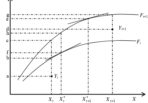
Theoretical Framework. Productivity re-fers to the rate at which production factors are transformed into output. Enhancement of pro-ductivity happens when more output results from given levels of inputs, or alternatively when the same level of output results from lower levels of inputs. Following Kalirajan’s (2004) approach of decomposition of total factor productivity, the general structure of the primal approach is illustrated in Figure 1, in which a single output is produced using a sin-gle input 2.
a b c d e
Yt+1
Yt
t
X Xt1 X
Y
t
X Xt1
f
g Ft+1
Ft
h
2
.Figure 1. Decomposition of output growth with inefficient producers
2 In Kalirajan’s decomposition, the producer is assumed to be allocatively efficient. Thus the technical efficiency actually
Let Y be a single output produced using a single input X with production technology F. At time t, the production frontier is Ft. The
level of Yt is produced using Xt. The
produc-tion is technically inefficient and allocaproduc-tion of input is still below allocatively efficient level. At time t+1, the production frontier moves upward from Ft to Ft+1. The level Yt+1 is pro-duced using Xt+1 with a new production fron-tier, but it is more technically efficient than before because the actual level of Yt+1 is closer to the production frontier, but allocation input exceeds allocatively efficient level. The in-crease in output from Yt to Yt+1 represents out-put growth. At time
t
, suppose the allocatively efficient level of input use is Xt* where themarginal product of the input is equal to the relative price of the input. At time t+1, the allocatively efficient level is Xt*1 where the
marginal product of the input is equal to its relative price. The rate of output growth is
1
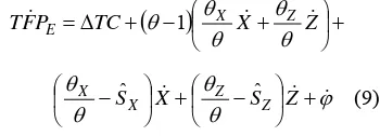
Scale effects resulting from input growth need to be taken into account. Total factor productivity growth is output growth unex-plained by input growth, and then total factor productivity growth is expressed as:
SE the production technology exhibits constant, increasing or decreasing returns to scale, the effect will be zero, positive or negative re-spectively.
From the neoclassical growth proposed by Solow (1957), the growth of output is mathe-matically decomposed as:
Z
the observed share of input Z expenditure, and WXand WZ are prices of input X and Z
respectively. The rate of change in technology
is represented by
ductivity growth can be defined as the growth in output which is unexplained by growth in inputs, that is:
In this case, total factor productivity growth is the same as the rate of technological progress. Chen (1997) points out that this de-composition of productivity growth is the same as the growth accounting approach be-cause Solow (1957) makes assumptions of Hicks-neutral technological change and con-stant returns to scale production technology. Another assumption not accounted for is tech-nical and allocative efficiency in producing outputs.
production frontier with environmentally det-rimental input
X
and conventional inputZ
, technology parameter vector , time trendt
as a proxy for technological change, and output-oriented technical inefficiencyu
≥ 0 is repre-sented as:
it it
itit f X Z t u
Y , ,; exp (5)
Technical efficiency is expressed as
exp
1allows it to vary over time. A primal measure of the rate of change in technical efficiency is given as: producer shifts towards or away from the pro-duction frontier, keeping everything else con-stant. Taking log and totally differentiating equation (5) and then differentiating with re-spect to
t
, yield:of the stochastic production frontier,
is the rate of technological
change, X
is output elasticity with
respect to input X,
Zelasticity with respect to input Z,
in technical efficiency. Substituting the ex-pression for Y into equation (4) yields: provides a primal measure of returns to scale of the production frontier. The notation of
X
and Z
is called normalised output
elas-ticity with respect to input X and Z respec-tively. The effect of returns to scale is repre-sented by notation of
1
, which will be positive, negative, or zero if the production technology exhibits increasing, decreasing or constant returns to scale respectively. Alloca-tive efficiency of input use will be reached if normalised output elasticity with respect to all inputs is equal to the share in cost of the respective inputs; in other words,MRTS
is equal to the price ratio of inputs.This decomposition of total factor pro-ductivity is able to break down economic effi-ciency, as proposed by Bauer (1990), into al-locative and technical efficiency. It can be seen in equation (6.10) that total factor pro-ductivity growth is decomposed into the com-ponents of technological change, scale effect, allocative efficiency, and technical efficiency3.
3 If there is no technological change or change in the
Internalization of Environmental Cost.
Chemical inputs have been known to be envi-ronmentally detrimental. Using chemical in-puts where producers are technically ineffi-cient will discharge extra pollution, leading to environmental cost. Pretty & Waibel (2005) point out that the environmental costs associ-ated with agrochemicals should be internalised into production costs. When environmental cost is considered as a production cost in analysis of economic production, it should be included in the cost of the detrimental input. Internalising environmental cost into the cost of inputs will raise the production cost of puts. The increase in production cost will in-fluence allocative efficiency. After taking en-vironmental costs into account, the outcome is considered as social efficiency (Grafton, et al., 2004; Pearce & Turner, 1990; Tietenberg, 1998). The component of allocative efficiency in the decomposition of total factor productiv-ity will change, because of changes in the share of input expenditure. The share of
ex-penditure for input X will be
the environmental cost associated with ineffi-ciency of environmentally detrimental input use. Consequently, the decomposition of
Allocative inefficiency is represented by the deviations in normalised output elasticity and share of input cost. When all the gaps are zero, the uses of all the inputs are allocatively efficient, and there is no effect on total factor productivity growth. Lastly, if there is zero growth in inputs, the scale and allocative efficiency component will be zero, the growth in total factor productivity is only driven by technological change and technical efficiency. Therefore, if farms are always allocatively and technically efficient and the production technology has constant returns to scale, the total factor productivity growth is equal to the rate of improvement in technology or technological change. This is consistent to technological change proposed by Solow (1957).
ronmentally adjusted total factor productivity will be:
where TFPE represents environmentally ad-justed total factor productivity growth.
Internalising environmental cost therefore, could have either a positive or a negative ef-fect, depending on the current position of allo-cative efficiency. The difference between total factor productivity growth with and without internalisation of environmental cost can be considered the rate of reduction of agricultural productivity associated with the negative ef-fect of agro-chemical use.
Data and Variables. This study uses a database which is established from a longitu-dinal survey conducted by the Indonesian Centre for Agricultural, Socioeconomic and Policy Studies (CASEPS) of the Ministry of Agriculture. The database is unbalanced panel data consisting of 358 farm operations in Indonesia during 1994, 1999 and 2004. The sample is collected from five regions. Some villages are selected in each province and farmers cultivating rice are sampled randomly. Once farmers are selected, they become respondents of the survey and are interviewed every five years. The total number of observa-tions used is 817.
most farmers are interviewed in the periods 1994 and 2004, and 1994, 1999 and 2004. In addition, more than two thirds of total sampled farmers are interviewed twice with five-year and ten-year intervals, and the rest are inter-viewed three times with five-year intervals.
The number of variables observed in the data collection done with interviewing sam-pled farmers varies widely. This is because the survey is accommodating variations in which farming is very spatially and temporally spe-cific. For example, certain fertilisers are not used in one place and always used in another place. In some regions, it is usual that there is voluntary labour during early planting and harvesting seasons, but this not the case in others. As well, some farmers are able to sepa-rate expenses of rice agriculture in some de-tail, but some others are not. For the purpose
of this study, however, the data are then ag-gregated to avoid problems of missing data3.
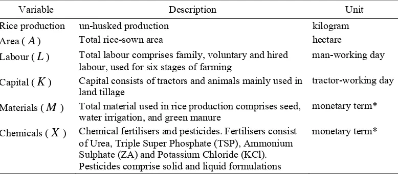
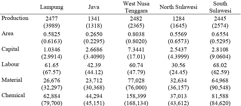
The description and measurement of aggregated variables of input-output and technical inefficiency models from individual observations are given in Table 3. Table 4 shows the summary statistics for key variables across time. Table 5 shows summary statistics for key variables sorted by region. On average, production increases over time. Area, along with materials and agrochemicals grow over time. But there is a considerable slowdown in capital use. Labour increases almost two-fold in 1999, but decreases in 2004. It is important to note that standard deviation of each variable in each region is relatively high, indicating that there is considerable variation in such variables. We can see that, on average, the highest rice production is in West Nusa Teng-gara, with the largest area of rice-sown land.
Table 3.4Data on input and output of rice agriculture
Variable Description Unit
Rice production un-husked production kilogram
Area (
A
) Total rice-sown area hectareLabour (
L
) Total labour comprises family, voluntary and hired labour, used for six stages of farmingman-working day
Capital (
K
) Capital consists of tractors and animals mainly used in land tillagetractor-working day
Materials (
M
) Total material used in rice production comprises seed, water irrigation, and green manuremonetary term*
Chemicals (
X
) Chemical fertilisers and pesticides. Fertilisers consist of Urea, Triple Super Phosphate (TSP), Ammonium Sulphate (ZA) and Potassium Chloride (KCl). Pesticides comprise solid and liquid formulationsmonetary term*
Note: *) Monetary value is at 1993 constant price
4 In agricultural practice, including rice agriculture, it is typical that farmers do not use fertilizers, pesticides and tractors.
Table 4. Summary statistics for key variables, by year
1994 1999 2004
mean standard
deviation mean
standard
deviation mean
standard deviation
Production 1,856 1,751 2121 2866 3,445.11 3,972
Area 0.55 0.53 0.62 0.60 0.88 0.95
Capital 8.19 17.12 1.45 2.59 0.44 2.26
Labour 41.69 35.34 78.99 59.79 57.77 70.29
Material 35,503 39,247 58,580 60,884 81,322 109,758
Chemical 52,414 54,709 64,896 71,210 254,891 2,255,989
Note: See Table 3 for units of measurement. Source: Author’s calculation
Table 5. Summary statistics for key variables, by region
Lampung Java West Nusa
Tenggara North Sulawesi
South Sulawesi
Production 2477
(3989)
Capital 1.0346
(2.9914)
Material 26,676
(32,297)
Chemical 62,884
(79,700)
Note: Figures in parentheses represent standard deviations. See Table 3 for units of measurement. Source: Author’s calculation
Production Technology. By now, after introduction of transcendental logarithmic (translog) production technology by Christen-sen, et al. (1973), it becomesthe fashionable functional form of a production function in estimating total factor productivity is the (Chen, 1997).5 The stochastic frontier translog production technology is specified as:
5 The work of Thiam et al. (2001) concludes that using
more flexible functional forms results in more accurate technical efficiency estimate. More flexible functional forms reduce the error terms (itvituit), which means higher estimates of technical efficiency. Considering that a higher rate of efficiency represents a
The full translog production technologies captures more accurate estimates and more
precise technical efficiency, which will be subsequently used for calculating decomposi-tion of productivity growth of rice producdecomposi-tion.
Given the estimated parameters in the production function, the mean elasticities of output with respect to inputs are formulated as:
The elasticity of production with respect to input
X
i is expressed as:The mean output elasticities are then evaluated at the average level of each input and time period. The rate of technological change is defined as the percentage change in output due to an increment of time in which all inputs are held constant, that is:
t
The rate of technological change consists of two components. First, biased technological
change shown by
pure technological change shown by
t
tt
t
2
. The biased technological change
is producer specific, and, in contrast the pure technological change will be constant, in-creasing or dein-creasing at a constant rate, ac-cording to whether tt is zero, positive or
negative respectively.
Following Cornwell, et al. (1990) the tem-poral pattern of technical efficiency is mod-elled as a quadratic function of time, that is:
2
The rate of change in technical efficiency is:
t
Input growth is considered to vary over time. The rate of growth of input is estimated using the expression:
r1 2 represents non-constant rate of input growth. Taking logarithm of both right and left hand sides gives log linear expressions:
2
and this can be easily estimated using OLS. The rate of input growth is obtained as:
t
Environmental cost associated with the use of environmentally detrimental inputs is estimated using an effect on production ap-proach (Garrod and Willis, 1999), that is the value of output that must be given up to mini-mise pollution or chemical waste. Since using the environmentally detrimental inputs pro-vides benefits to producers in terms of in-creased output for a given level of inputs (Paul, et al., 2002), it is reasonable to make an inverse statement of the effect on production as follows: environmental cost is the monetary value of output that must be given up in order to maintain minimum pollution. Given the estimated production function, the minimum environmental cost associated with the amount of environmentally detrimental input dis-charged into the environment can be calcu-lated as:
f X Z f X Z
P
EC act, min, (18)
where P is prevailing price of output (see Mariyono, et al., 2010 for detail in estimating environmental cost).
RESULTS AND DISCUSSION
tech-nology, the four components of total factor productivity are calculated. The first compo-nent is technological change, which consists of non-neutral and pure effects. The second com-ponent is rate of change in technical effi-ciency. Both components are described in Ta-ble 7. The next two components are: scale
effects, which involve output elasticity with respect to each input and input growth of re-spective input; and allocative efficiency, which involves share in input costs without environmental cost and with environmental cost.
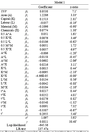
Table 6. Parameter estimates of stochastic frontier production function
Model 1
Coefficient z-ratio
TFP 0 8.0538 7.1a
Area (A) 1 1.2286 3.33a
Capital (K) 2 0.1513 2.81b
Labour (L) 3 -0.057 -0.19n
Material (M) 4 -0.1096 -0.98n
Chemicals (X) 5 0.0774 1.38n
0.5 A*A 11 0.051 1.61c
0.5 K*K 22 0.0076 3.49a
0.5 L*L 33 -0.0106 -0.62n
0.5 M*M 44 0.0051 1.72c
0.5 X*X 55 0.0057 6.97a
A*K 12 -0.006 -1.20n
A*L 13 -0.0158 -0.45n
A*M 14 -0.0602 -2.06b
A*X 15 0.0216 3.11a
K*L 23 0.0015 0.44n
K*M 24 -0.0095 -2.18b
K*X 25 -4.66E-05 -0.08n
L*M 34 0.0134 0.56n
L*X 35 -0.0042 -0.88n
M*X 45 -0.0104 -2.10b
t*A 1t 0.0217 0.44n
t*K 2t 0.0252 4.81a
t*L 3t 0.0276 0.82n
t*M 4t -0.0548 -1.32n
t*X 5t 0.0891 7.32a
t t -0.3387 -0.67n
t2 tt 0.2955 5.48a
2
1.097 5.92a
0.8811 38.48a
Log-likelihood -645.56 LR-test 137.47a
Note: Dependent variable: output (kg); all variables are logarithmic form; a) significant at
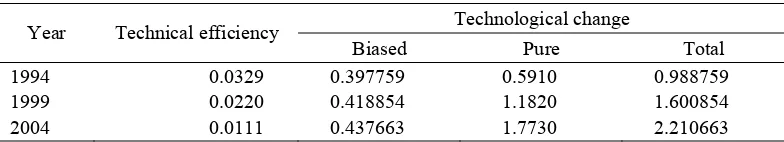
Table 7. Rate of change in technical efficiency and technological change
Technological change
Year Technical efficiency
Biased Pure Total
1994 0.0329 0.397759 0.5910 0.988759
1999 0.0220 0.418854 1.1820 1.600854
2004 0.0111 0.437663 1.7730 2.210663
The estimated translog production tech-nology shows that is highly significant. This means that there is significant deviation of actual output to potential output which is brought about by technical inefficiency. In other words, the average translog production technology is significantly less than the fron-tier.
Technological change relates to time trend in the frontier production technology. A joint test for neutral technological change and pure technological change is rejected. This indi-cates that there are movements in production frontiers across time, representing technologi-cal change. The temporal pattern of estimated technical efficiency is represented as:
2
0054 . 0 0438 . 0 6177 .
0 t t
it
(19)
The joint test for time-invariant technical effi-ciency shows that F3562 3.85; and it rejects at 5 per cent significance, meaning that technical efficiency is not time-invariant. Technical ef-ficiency increases at a decreasing rate. The rate of change in technical efficiency is esti-mated as:
t T
it
it
0.0438 0.0109
(20)
The rate of change in technical efficiency and technological change in each year is given in Table 7.
The rate of change in technical efficiency in 1994, 1999 and 2004, was 0.0329, 0.0220 and 0.0111 respectively. The rate of change in non-neutral technological change is positive but increasing, meaning that, technological change is, in total, input augmenting. The im-plication is that technological change leads to
increases in input use. The rate of change in pure technological change is positive and in-creasing.6 This indicates that given the same level of input use, rice production increases over time. This implies technological progress in Indonesian rice agriculture during the peri-ods of 1994, 1999 and 2004. In total, techno-logical change is positive and increasing. The impressive growth in technological change is an indication that farmers have adopted better technology in rice production, and this ex-plains why the rate of change in technical effi-ciency is low.7 The technological change that account for innovation and diffusion of agri-cultural technology can provide a significant multiplier effect on other sectors (Khan & Thorbecke, 1988).
Scale effect and allocative efficiency re-late to output elasticity with respect to each input. The output elasticity derived from translog production technology is not constant and dependent on the level of each input use. The output elasticity, which is calculated at the average level of each input use, is shown in Table 8. Together with input growth, the aver-age output elasticity in each year will be used to calculate scale effect and allocative effect. Input growth is estimated using regression of the logged input on quadratic time trends. The result of the regression is given in Table 9.
6 A high rate of technological progress with a similar
pattern of technological change has been shown by Villano & Fleming (2006) for rice agriculture in the Philippines.
7 Jansen & Ruiz de Londono (1994) mention that
As mentioned above, input growth is expected not to be constant over time. All regressions are highly significant in overall tests, despite the fact that some coefficients are individually insignificant. This is because the time series trend is only three, and unbalanced.
This condition leads to a strong correlation between linear and quadratic trends, resulting in a multicollinearity problem (Wooldridge, 2003). The rate of input growth of each input is given in Table 10.
Table 8. Output elasticity with respect to each input
Year Inputs
1994 1999 2004 Total
Land 0.7207 0.6969 0.7432 0.7166
Capital 0.0343 0.0487 0.0315 0.0443
Labour 0.0000 0.0000 0.0000 0.0000
Material 0.1043 0.1028 0.1229 0.1077
Chemicals 0.0013 0.0884 0.1920 0.0923
Scale elasticity 0.8605 0.9368 1.0896 0.9608
Note: the output elasticity is evaluated at the average of all (ln) input use in 1994, 1999, 2004 and total.
Table 9. Regression of input (in logarithmic form) on time trend
Dep. Var. Constant t 2
t
Coef. -0.9473 -0.0899 0.0649 F=7.39a
ln Land
t-ratio -4.03a -0.33 0.93 R2=0.02
Coef. -10.6166 6.6654 -2.4319 F=45.66a
ln Capital
t-ratio -5.97a 3.21a -4.59a R2=0.10
Coef. 1.3770 2.6447 -0.6430 F=54.16a
ln Labour
t-ratio 6.17a 10.16a -9.68a R2=0.12
Coef. 8.6592 1.4895 -0.2854 F=16.37a
ln Material
t-ratio 21.51a 3.17a -2.38a R2=0.04
Coef. 7.2044 -1.6099 0.6750 F=11.22a
ln Chemicals
t-ratio 5.79a -1.11 1.82c R2=0.03
Note: a) significant at 5%, c) significant at 10%
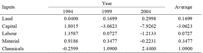
Table 10. Rate of input growth (five-yearly)
Year Inputs
1994 1999 2004 Average
Land 0.0400 0.1699 0.2998 0.1699
Capital 1.8015 -3.0623 -7.9262 -3.0623
Labour 1.3587 0.0727 -1.2133 0.0727
Material 0.9186 0.3477 -0.2231 0.3477
On average, inputs grow, except capital which decreases at 306 per cent during the period. Capital consisting of tractors and ani-mals, dropped sharply because the economic crisis in 1997/1998. Agricultural machinery becomes more significantly expensive after the crisis. The highest rate of positive growth is agrochemicals, more than 100 per cent dur-ing the same period. In 1994, the rate of growth of all inputs was positive, except agro-chemicals which declined at the rate of 26 per cent. The highest rate of growth was capital at 180 per cent. However, in the next period, the rate of capital growth drastically felt. On the other hand, agrochemicals dropped in 1994, while the rate of growth in 1999 and 2004 rose considerably. Labour and material inputs have the same pattern, initially high rates of growth, and then the rate falls in the next two periods, and becomes negative in 2004. The rate of land growth is continually positive and in-creasing over time.
The rate of input growth will contribute to scale effects and allocative efficiency effects. Scale effects are determined in three compo-nents: input growth, as it has been previously discussed; returns to scale, the sum of output elasticity with respect to all inputs; normalised elasticity, the ratio of output elasticity with respect to each input to the sum of output elasticity with respect to all inputs. As shown in Table 8, the translog production technology
of rice agriculture exhibits decreasing returns to scale in 1994 and 1999, and increasing re-turns to scale in 2004. Overall, however, the production technology exhibits decreasing returns to scale. The normalised elasticity re-sulting from output elasticity with respect to each input is given in Table 11.
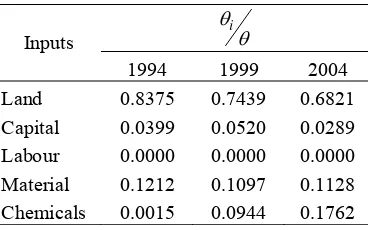
The normalised output elasticity of each input has a similar pattern to the output elasticity. The important difference between normalised elasticity and output elasticity is that the sum of normalised elasticity is exactly equal to unity. The scale effect is given in Table 12. The scale effect in the first two points in time is negative. This is because there is decreasing returns to scale in those periods. In contrast, the scale effect is positive in the last point in time, because of increasing returns to scale.
Table 11. Normalised output elasticity
i
Inputs
1994 1999 2004
Land 0.8375 0.7439 0.6821
Capital 0.0399 0.0520 0.0289
Labour 0.0000 0.0000 0.0000
Material 0.1212 0.1097 0.1128
Chemicals 0.0015 0.0944 0.1762
Table 12. Rate of change in scale effect and its components (five-yearly)
i i
X
Inputs
1994 1999 2004
Land 0.033501 0.126391 0.204489
Capital 0.071809 -0.1592 -0.22914
Labour 0 0 0
Material 0.111342 0.038155 -0.02516
Chemicals -0.00039 0.102857 0.429956
i i
iX
0.21626 0.108208 0.380137
1
-0.1395 -0.0632 0.0896 i i
iX
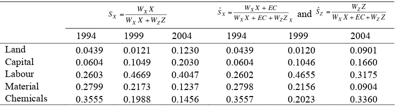
The last component of total factor pro-ductivity growth is the allocative efficiency effect, which constitutes the gap between the normalised output elasticity and share in input cost. In this analysis, share in input cost is sorted into private cost and social costs. The private cost of input is the cost for which envi-ronmental cost associated with environmen-tally detrimental inputs is not taken into ac-count. Conversely, the social cost of input is the cost for which environmental cost is inter-nalised as input cost. Since the environmental cost is a negative externality, the social cost will be greater than the private cost. The share in both private and social costs is given in Ta-ble 13.
Let us first describe the share in private costs. Generally, labour and agrochemicals have a higher share in cost of production. In small-scale rice agriculture, this condition is reasonable. Small-scale rice agriculture is usu-ally labour and chemical intensive. Chemicals are used to increase productivity of land, and labour is more suitable than tractors. This cor-responds to the low share in cost of capital which is a less suitable input in small-scale rice agriculture. Land has the smallest share in cost, because most farmers studied here oper-ate rice agriculture on their privoper-ately owned land. The cost related to land is land tax, which is relatively low in rural areas. The shares of land, labour and capital costs tend to increase, whereas the shares of agrochemicals and materials tend to decease. The dynamics of shares of cost is dependent on the price of
inputs, and the level of use of these inputs.
With respect to share of social cost, it is theoretically expected that the share of chemi-cal cost increases and the share of other input cost decreases. This is because the environ-mental cost associated with agrochemicals, which is considered to be environmentally detrimental, is internalised into the cost of chemical inputs. In the first two points in time, the impact of internalisation of environmental cost is very low. But, in the last point in time, there is considerable change in those shares. This is an indication that in the last point in time, the environmental cost associated with chemical input is significant.
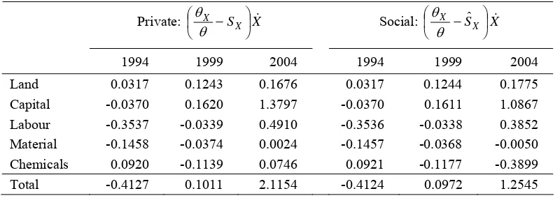
With positive rate of growth in inputs, al-locative efficiency effect will be positive, negative or zero if the gap resulting from nor-malised output elasticity with respect to each input minus the share in cost of the corre-sponding input is positive, negative or zero respectively. The gap between normalised output elasticity with respect to each input is shown in Table 14.
Allocative and social efficiencies are not the case here, and therefore allocative and so-cial efficiency effects will affect the total fac-tor productivity growth. Land has a positive gap, meaning that the use of land is low com-pared with other inputs. The gap decreases over time due to the increase in land tax. Capital, labour and materials have a negative gap. This means that the use of these inputs is economically excessive relative to land use.
Table 13. Share in cost of input use
Z W X W
X W S
Z X
X
X
X Z X
X
X W X EC WZ
EC X W S
ˆ
and W X EC W Z
Z W S
Z X
Z
Z
ˆ
1994 1999 2004 1994 1999 2004
Land 0.0439 0.0121 0.1230 0.0439 0.0120 0.0901
Capital 0.0604 0.1049 0.2030 0.0604 0.1046 0.1660
Labour 0.2603 0.4669 0.4047 0.2602 0.4655 0.3175
Material 0.2799 0.2173 0.1237 0.2798 0.2156 0.0904
The negative gap for capital increases, whereas the negative gap for materials de-creases over time and the gap for labour fluc-tuates. Chemicals have a negative gap in 1994 and become positive in the next two periods. After internalisation of the environmental cost associated with inefficient use of agrochemi-cals, the gaps change slightly. As expected, the gaps for land, capital, labour and materials increase because the shares of cost of these inputs fall. In contrast the gap for agrocals increases since the share of cost of chemi-cal inputs becomes higher after internalisation of the environmental cost.
We can see that there is improvement in overall allocative efficiency as well as social efficiency. After internalisation of the envi-ronmental cost associated with inefficient use of agrochemicals, the gaps change slightly. As expected, the gap for land, capital, labour and
material increase because the shares of cost of these inputs fall. In contrast the gap for agro-chemicals increases since the share of cost of chemical inputs becomes higher after inter-nalisation of the environmental cost. The gaps will have total impacts on the total factor pro-ductivity growth if there is variation in input growth. As shown in Table 10, there is varia-tion in input growth. The total allocative and social efficiency effects are given in Table 15.
Land and capital have positive allocative efficiency effects. This is because the gap for land is positive and land use grows positively. In 1994, capital has a negative allocative effi-ciency effect, after which the effect increases considerably. The considerable increase in allocative efficiency effect is due mostly to drastic falls in capital growth. Since the use of capital is no longer allocatively efficient, the negative growth causes allocative efficiency to
Table 14. Average gap between normalised output elasticity and share of input cost
Private: X SX
Social X SˆX
1994 1999 2004 1994 1999 2004
Land 0.7936 0.7318 0.5591 0.7937 0.7319 0.5920
Capital -0.0205 -0.0529 -0.1741 -0.0205 -0.0526 -0.1371
Labour -0.2603 -0.4669 -0.4047 -0.2602 -0.4655 -0.3175
Material -0.1587 -0.1075 -0.0109 -0.1586 -0.1059 0.0224
Chemicals -0.3540 -0.1045 0.0306 -0.3542 -0.1079 -0.1598
1.5871 1.4636 1.1794 1.5872 1.4638 1.2288Table 15. Average rate of change in allocative efficiency effect (five-yearly)
Private: SX X
X
Social: SX X
X
ˆ
1994 1999 2004 1994 1999 2004
Land 0.0317 0.1243 0.1676 0.0317 0.1244 0.1775
Capital -0.0370 0.1620 1.3797 -0.0370 0.1611 1.0867
Labour -0.3537 -0.0339 0.4910 -0.3536 -0.0338 0.3852
Material -0.1458 -0.0374 0.0024 -0.1457 -0.0368 -0.0050
Chemicals 0.0920 -0.1139 0.0746 0.0921 -0.1177 -0.3899
rise. For the case of labour and materials, the allocative efficiency effects are negative in the first two points in time, but the effects in-crease. In 2004, the rate of labour and material growth was negative and at the same time there was an increase in cost of labour and materials resulting in decrease in allocative efficiency. For the case of labour, the increase was relatively high because the fall in labour growth was very high. For the case of agro-chemicals, the effect of allocative efficiency was positive and increasing. In 1994, agro-chemicals decreased and the gap was negative. In the next two points in time, both growth and gap were positive. The total effect is positive.
The allocative and social efficiency effects are considerable. The effects increase over time starting from a negative value. This indi-cates that there is improvement in allocative efficiency as well as social efficiency effects, particularly after the economic crisis in 1997/1998. The allocation of inputs is much more efficient after the crisis. Farmers become more conscious if some inputs are incorrectly allocated. They will adjust the use of inputs based on the productivity of such inputs.
Internalising environmental cost into cost of chemical input reduces the total impact. In 1994 and 1999 the decrease was quite small, but in 2004 there was a dramatic decrease in total impact of allocative efficiency, which dropped from 4.3712 to 3.5103. The sharp
decrease resulting from the internalisation indicates very high environmental costs.
Table 16 shows the total factor productiv-ity growth, which stems from growth in tech-nological change, scale effect, allocative effi-ciency and technical effieffi-ciency. In absolute value, the total factor productivity growth is high, particularly for 2004. The largest con-tributor to total factor productivity growth is technological change, followed by the alloca-tive efficiency effect, which comes from allo-cative efficiency and growth of inputs. With respect to the considerable magnitude of total factor productivity growth, it could be accept-able for the following logical reason. The time interval is five years, which is relatively long. If the total factor productivity growth is taken in yearly accounting, the growth becomes 0.1157, 0.3434 and 0.8742 for 1994, 1999 and 2004 respectively.
Based on this finding, technological change and allocative efficiency effects are the significant components of total factor produc-tivity growth. In the previous studies on pro-ductivity growth using stochastic production technology which do not account for allocative efficiency effects, the estimates of total factor productivity growth are misleading. It could be an underestimation or overestimation, which is dependent on the level of allocative efficiency and input growth. Thus, in the pre-vious studies, those effects are still unex-plained.
Table 16. Source of total factor productivity growth of rice agriculture (five-yearly)
Conventional Environmentally adjusted
Component
1994 1999 2004 1994 1999 2004
TC 0.9888 1.6009 2.2107 0.9888 1.6009 2.2107
Scale -0.0302 -0.0068 0.0341 -0.0302 -0.0068 0.0341
AE -0.4127 0.1011 2.1154 -0.4124 0.0972 1.2545
TE 0.0329 0.0220 0.0111 0.0329 0.0220 0.0111
TFP 0.5787 1.7171 4.3712 0.5791 1.7132 3.5103
This study shows impressive growth in total factor productivity. Slow growth in 1994 was due to ignorance of the agricultural sector at the time (Mellor, et al., 2003). Since the economic crisis, the sector has become more central because of the fact that it is the only sector able to grow in the economic crisis. After that, the sector has had much more attention from the government, resulting in high growth in total factor productivity.
Productivity growth changes after inter-nalisation of environmental cost into the cost of chemical inputs. The effect of internalisa-tion of environmental cost is to increase total factor productivity growth for 1994. The posi-tive impact of internalisation is due to an aver-age improvement in allocative efficiency of input uses. In contrast, the effect of internali-sation of environmental cost is to decrease total factor productivity growth for 1999 and 2004. The negative impact of internalisation is due to an average decrease in allocative effi-ciency of input uses. In 1994 and 1999 the change in total factor productivity growth re-sulting from internalisation of environmental cost was small, but in 2004 the change was very high. Overall, the impact of internalisa-tion of environmental cost into the cost of in-puts is to decrease total factor productivity growth.
It seems that the statement of Kalirajan, et al. (2001) — growth in productivity of agri-cultural production in some developing coun-tries is decreasing due partly to environmental degradation — is in line with this outcome. This is supported by Toruel & Koruda (2004) who highlight that technological change in Asian agriculture was exceptional, when the Green Revolution began, but has decreased sharply since. In the era of the Green Revolution, the use of agrochemicals is excessive and tends to be inefficient (Pimentel, et al., 1993). For the case of Indonesian rice agriculture, the main cause of excessive use of agrochemicals is government subsidy (Conway & Barbier, 1988; Barbier,
1989). The excessive use of agrochemicals leads to environmental degradation, particu-larly land degradation, resulting in falls in soil fertility and, eventually, decreases in produc-tivity of agriculture.
The total factor productivity growth after internalisation of environmental cost can be considered as the environmentally adjusted growth of total factor productivity. This meas-ure is to some extent important because of current concerns of the global community re-garding environmental protection. If the target of agricultural policy is to increase the envi-ronmentally adjusted growth, it will not jeop-ardise environmental quality much, particu-larly in the agricultural sector. The environ-mentally adjusted growth of total factor pro-ductivity can be enhanced by improving the rate of change in technical efficiency, techno-logical change, scale effect and allocative effi-ciency effect.
changes in shares then influence the social efficiency effect.
The case of scale effect, which also varies, needs careful policy formulation. Given the parameters of rice production technology, the scale effect can be improved by reducing or increasing the use of inputs. Referring to the increasing returns to scale of production tech-nology in 2004, it is reasonable to increase the use of land, labour and chemical inputs which have positive normalised elasticity, and to reduce the use of capital and material inputs which have negative normalised elasticity.
However, the increase in use of inputs also influences social efficiency. For 2004, the increase in land use leads to increased social efficiency, but the increases in other inputs lead to decreased social efficiency. It is there-fore, the increase in land use which will im-prove scale and social and allocative effi-ciency effects. The increases in both effects can also be achieved by reducing capital and material inputs. The increases in labour and chemical inputs will lead to opposite impacts on scale and social efficiency effects. The policy that is able to provide greatest net posi-tive impact is preferable.
CONCLUSION
Indonesian rice agriculture needs to grow in order to be capable of keeping pace with the rising need for food of the national population to ensure national food security. Enhancing productivity does not mean jeopardising envi-ronmental quality, however, and formulating sustainable agricultural productivity growth is crucial, since agricultural growth in develop-ing countries shows a discernible decline. Two possible main reasons are no major break-throughs in developing agricultural technol-ogy, and a decline in the quality of the envi-ronment and land. Lack of technological pro-gress and deterioration in productive resources are crucial factors that slow agricultural growth. Thus analyses on “green” productivity growth are needed to recognise the sources of
productivity and the impact of taking envi-ronmental problems into account.
Using an approach of total factor produc-tivity growth, which is decomposed into tech-nological change, technical efficiency, scale effect and allocative efficiency effect, the total factor productivity growth of rice agriculture is determined. Environmental cost, associated with the inefficient use of agrochemicals is then internalized. Without taking environ-mental cost into account, the rate of growth in total factor productivity was low in 1994, but quite high in 1999 and 2004. Mostly, the rate of growth in total factor productivity is driven by an impressive rate of growth in technologi-cal change, followed by improvement in allo-cative efficiency effect. The high productivity growths in 1999 and 2004 were due to recov-ery from the economic crisis. Farmers have better allocated inputs.
After taking the environmental cost into account, the rate of growth in total factor pro-ductivity, overall, decreases. This is called environmentally adjusted total factor produc-tivity growth or “green growth”. The growth is less than usual because the shares in costs of all inputs change and, consequently, allocative efficiency effects change as well. A high change in the allocative efficiency effect oc-curred in 2004, and this change reduced the rate of growth in total factor productivity by around 40 per cent. This is an indication of which environmental cost associated with the use of chemical inputs is significant.
POLICY IMPLICATION
con-ducted by sending farmers in agronomic training. Many studies show that agronomic training equipping farmers with knowledge and practices has enhanced farming efficiency.
Another policy that can improve produc-tivity growth is to increase cultivated land area, which improves scale and social effi-ciency effects. Even though this is not an easy task because of massive agricultural land con-version in Java, land expansion can still be possible out-side Java where land is still avail-able. In Java, it could be carried out by utiliz-ing uncultivated land for dry land “gogo” rice farming. By now, seed technology has pro-vided better cultivars of rice suitable in dry land.
One important long-run policy is to reduce dependency of Indonesian people on rice as a staple food. Indonesian people need to diver-sify their foods. If this is achievable, there is no need land expansion in Java; even, rice farmers are likely to change rice with other higher valued crops such as horticultural crops. Changing rice farming to horticultural crops makes it possible for farmers to increase welfare (Mariyono & Bhattarai, 2011).
During the 1st presidency of Susilo
Bambang Yudhoyono, agricultural revitaliza-tion program fitted this implicarevitaliza-tion of study. Increasing agricultural land (including for rice) is conducted outside Java; various high yielding cultivars of rice have been released; and training programs on agriculture have been launched (Mariyono, 2009). Currently, Indonesian agency food security promotes food diversification to provide more choice for people to eat.
CAVEATS
This study uses panel data with intervals of five years, which is quite long. As a conse-quence, the data set is an unbalanced panel because of conditions such as farmers having died, no longer operating the rice farm, or having sold the paddy land. Using an
unbal-anced panel is somewhat less effective than a balanced panel data, but is better than using cross-sectional data. The latest data used in this study 2004, which is eight years ago. Newly set data is needed to understand the current condition.
The sample size of the longitudinal survey is, to some extent, small because of resource constraints. Consequently, the sample may not well represent the overall condition of Indone-sian rice agriculture. However, the sample is collected from the main islands of Indonesia, considered the rice bowl areas. It is expected that the sample is able to represent regional differences.
The sample is selected deliberately, that is, the selected rice growers are farmers spe-cialised in rice production, and the rice pro-duction is based on the optimal planting sea-son. The conditions, therefore, do not repre-sent average rice cultivation. Lastly, the pro-ducers are surveyed longitudinally, or, they are a permanent sample. It is likely that the pro-ducers will be influenced by the survey, such that they change behaviour related to agricul-tural practices. The change in behaviour may vary across producers. If the producers want to show that their own rice production has made good progress, they will improve their prac-tices. Conversely, if they want to get agricul-tural assistance, they will use worse practices. It is expected that the former offsets the latter, such that the behaviour is captured as white noise or disturbance error.
REFERENCES
Aigner, D.J., C.A.K. Lovell, and P. Schmidt, 1977. Formulation and Estimation of Stochastic Frontier Production Function Models. Journal of Econometrics, 6, 21-37.
Bauer, P.W., 1990. Decomposing TFP Growth in the Presence of Cost Inefficiency, Nonconstant Return to Scale, and Technological Progress. Journal of Pro-ductivity Analysis, 1, 287-299.
Belbase, K. and R. Grabowski, 1985. Techni-cal Efficiency in Nepalese Agriculture.
Journal of Development Areas, 19, 515-25.
Bond, J.W., 1996. How EC and World Bank
Policies are Destroying Agriculture and the Environment. Singapore: AgBé Publishing.
Chen, E.K.Y., 1997. The Total Factor Pro-ductivity Debate: Determinants of Economic Growth in East Asia.
Asian-Pacific Economic Literature, 11 (1), 18-38.
Christensen, L.R., D.W. Jorgenson, and L.J. Lau, 1973. Transcendental Logarithmic Production Frontier. Review of Econom-ics and StatistEconom-ics, 55 (1), 29-45.
Coelli, T.J., 1996. Measurement of Total Fac-tor Productivity Growth and Biases in Technological Change in Western Australia Agriculture. Journal of Applied Econometrics, 11, 77-94.
Conway, G.R. and E.B. Barbier, 1988. After the Green Revolution: Sustainable and Equitable Agricultural Development. Fu-ture, 20 (6), 651-670.
Garrod, G. and K.G. Willis, 1999. Economic Valuation of the Environment: Methods and Case Studies. Cheltenham: Edward Elgar Publishing, Inc.
Grafton, R.Q., W. Adamowicz, D. Dupont, H. Nelson, R.J. Hill S. and Renzetti, 2004.
The Economics of the Environment and Natural Resources. Carlton: Blackwell Publishing.
Hsieh, C., 2000. Measuring Biased Technolo-gical Change, available at http://www. wws.princeton.edu/~chsieh/Accessed on 20 June 2003.
Jansen, W. and N.R. Ruiz de Londonõ, 1994. Modernization of Peasant Crop in Co-lombia: Evidence and Implications. Ag-ricultural Economics, 10, 13-25.
Kalirajan, K.P., M.B. Obwona and S. Zhao, 1996. A Decomposition of Total Factor Productivity Growth: The Case of Chinese Agriculture Growth Before and
After Reforms. American Journal of
Agricultural Economics, 78, 331-338. Kalirajan, K.P., Mythili, G. and Sankar, U.,
2001. Accelerating Growth through
Globalisation of Indian Agriculture. New Delhi: MacMillan.
Kalirajan, K.P., 2004. An Analysis of India’s
Reform Dynamics. Oxford Development
Studies, 32(1), 119-134.
Khan, H.A. and E. Thorbecke, 1988. Macro Economic Effects and Diffusion of Alter-native Technologies with a Social Ac-counting Matrix Framework: The Case of Indonesia. Hants: Gower Publishing Co. Ltd.
Kong, X., R.E. Marks, and G.H. Wan, 1999. Technical Efficiency, Technological Change, and Total Factor Productivity Growth in Chinese State-Owned Enter-prises in the Early 1990s. Asian Eco-nomic Journal, 13(3), 267-281.
Kumbhakar, S.C. and C.A.K. Lovell, 2000.
Stochastic Frontier Analysis, Cambridge: Cambridge University Press.
Mariyono, J., 2009. Technological and Insti-tutional Changes of Indonesian Rice Sec-tor: From Intensification to Sustainable Revitalisation. Asian Journal of Agri-culture and Development, 6 (2), 125-144. Mariyono, J. and M. Bhattarai, 2011.
Surabaya: Indonesia Regional Science Association, 71-89.
Mariyono, J., B.P. Resosudarmo, T. Kompas. and Q. Grafton, 2010. Understanding Environmental and Social Efficiencies in Indonesian Rice Production. In: Beck-mann, V., N.H. Dung, X. Shi, M. Spoor, J. Wesseler (eds.), 2010. Economic Tran-sition and Natural Resource Manage-ment in East and Southeast Asia. Aachen: Shaker Verlag, 161-186.
Mellor, J.W., W.P. Falcon, D.M. Taylor, B. Arifin, E.G. Said, and E. Pasandaran,, 2003. Main Report of Agricultural Sector Review, Indonesia, Part I. CARANA Corporation, US Agency for International Development.
Michl, T.R., 1999. Biased Technical Change and the Aggregate Production Function.
International Review of Applied Eco-nomics, 13(2), 193-206.
Murgai, R., 2001. The Green Revolution and the Productivity Paradox: Evidence from the Indian Punjab. Agricultural Eco-nomics, 25, 199-209.
Nijkamp, P and G. Vindigni, 2000. Food Se-curity and Agricultural Sustainability: A Comparative Multi-country Assessment if Critical Success Factors. Tinbergen In-stitute Discussion Paper 070/3.
O”Neill, S. and A. Matthews, 2001. Technical Change and Efficiency in Irish Agri-culture. The Economic and Social Re-view, 32 (3), 263-284.
Paul, C.J.M., V.E. Ball, R.G. Felthoven, A. Grube, and R.F. Nehring, 2002. Effective Costs and Chemical Use in United States Agricultural Production: Using the Environment as a “Free” Input. American Journal of Agricultural Economics, 84 (4), 902-915.
Pearce, D.W. and R.K. Turner, 1990. Eco-nomics of Natural Resources and the En-vironment. New York: Harvester Wheatsheaf.
Pimentel, D., H. Aquay, M. Biltonen, P. Rice, M. Silva, J. Nelson, V. Lipner, S. Giordano, A. Horowitz and M. D’Amore, 1993. Assessment of Environmental and Economic Impacts of Chemical Pesticides Use. In: D. Pimentel and H. Lehmann (eds.), 1993. The Chemical Pesticides Question. London: Chapman & Hall, 47-84.
Sadoulet, E. And A. de Janvry, 1995. Quanti-tative Development Policy Analysis. Baltimore: John Hopkins University Press.
Shapiro, K.H., 1983. Efficiency Differentials in Peasant Agriculture and Their Implica-tions for Development Policies. Journal of Development Studies, 19, 179–190. Solow, R.M., 1957. Technical Change and the
Aggregate Production Function. Review of Economics and Statistics, 39, 312-320. Sun, C., 2004. Decomposing Productivity
Growth in Taiwan’s Manufacturing, 1991-1999. Journal of Asian Economics, 15, 759-776.
Teruel, R.G. and Y. Koruda, 2004. An Em-pirical Analysis of Productivity in Philip-pine Agriculture, 1974-2000. Asian Eco-nomic Journal, 18 (3), 319-344.
Thiam, A., B.E. Bravo-Ureta, and T.E. Rivas, 2001. Technical Efficiency in Develop-ing Country Agriculture: A Meta-analysis. Agricultural Economics, 25: 235-243.
Tietenberg, T., 1998. Environmental Eco-nomics and Policy. Reading: Addison Wesley.
Trewin, R., L. Weiguo, Erwidodo and S. Bahri, 1995. Analysis of the Technical Efficiency Over Time of West Javanese Rice Farms. Australian Journal of Agri-cultural Economics, 39 (2), 143-163. Tripp, R., 2001. Agricultural Technology
United Nations, 1997. Critical Trends: Global Changes and Sustainable Development. New York: UN Department for Policy Coordination and Sustainable Develop-ment.
Villano, R. and E. Fleming, 2006. Technical Inefficiency and Production Risk in Rice
Farming: Evidence from Central Luzon Philippines. Asian Economic Journal, 20 (1), 29-46.