REGRESSION ANALYSIS OF PRODUCTIVITY USING MIXED
EFFECT MODEL
Siana Halim, Indriati N Bisono
Faculty of Industrial Technology, Department of Industrial Engineering Petra Christian University, Surabaya
Email: {mlindri, halim}@petra.ac.id
ABSTRACT
Production plants of a company are located in several areas that spread across Middle and East Java. As the production process employs mostly manpower, we suspected that each location has different characteristics affecting the productivity. Thus, the production data may have a spatial and hierarchical structure. For fitting a linear regression using the ordinary techniques, we are required to make some assumptions about the nature of the residuals i.e. independent, identically and normally distributed. However, these assumptions were rarely fulfilled especially for data that have a spatial and hierarchical structure. We worked out the problem using mixed effect model. This paper discusses the model construction of productivity and several characteristics in the production line by taking location as a random effect. The simple model with high utility that satisfies the necessary regression assumptions was built using a free statistic software R version 2.6.1.
Keywords: mix effect model.
1. INTRODUCTION
One of production departments in a company employed mainly manpower in processing its products. Instead of having huge labors centered in one plant, the company built several production plants spread across Middle and East Java. This policy helps the company to raise efficiency, reduce overhead cost especially transportation cost, and ease to handle as the size of labors in each plant is relatively small.
According to the moving mechanism of products, production lines are categorized asynchronous. Basically the production lines are divided into two stations. Each station consists of groups of workers. In the first station, each group of three make the product by hand and tidy it as well as carry out the product quality control. In the second station, each group of two does the filling, labeling and packaging.
caused by each plant characteristics or environmental conditions while the within cluster variation reflects the random variation caused by uncertainty that cannot be explained by such plant characteristics.
This study is organized as follows. In Section 2, the data and the proposed model are presented. The case of that is discussed in Section 3. In the last section, some conclusions of this study are drawn with possible further studies.
2. METHOD
The collected data turn out a special challenge for statistical analysis for several reasons. First, the data have a spatial structure; they were collected from several locations. Second, they are temporal data, thus they might not independent. Third, the data consist of multicollinearity. Therefore the assumptions about the nature of the residuals i.e. independent, identically and normally distributed in fitting a linear regression using the ordinary techniques are hardly to fulfill. In dealing with the problem, we may apply mixed effects model as one of the solutions.
The linear mixed model (Harville, 1977; Laird and Ware, 1982) can be written as follows
i
unobservable random effects, and eidenotes an ni×1 vector of unobservable within-subject error
terms. The assumptions hold for this model is that bi has a multivariate normal distribution Nq(0,
G) independent of ei, which has a multivariate distribution Nni(0, Ri).
matrix for the within-subject error terms.
Harville (1977) discussed the use of maximum likelihood (ML) and restricted or residual maximum likelihood (REML) approaches for solving model (1). Laird and Ware (1982) proposed the use of the expectation-maximum (EM) algorithm to estimate the parameters.
In this study we use R version 2.6.1 to help us fitting the model. Model fitting in R and Splus is detailed by Pinheiro and Bates (2000).
2.1 Data and variables
In this section, we apply the proposed approach to the productivity based on data from 35 plants evaluated during 2006. The data contain the information about production as well as quality characteristics such as the production rate, the output per group hour, overhead cost per unit, level of waste in relation to input of raw materials, ratio of plant sizes to the number of working groups, ratio of experienced worker and inexperienced worker, the percentage of non-permanent employment contracts, the expenditure of health and safety at work and the percentage of presence.
2.2 Models
Prior to fit a production rate prediction model using the data, we employed Stepwise regression to remove and add variables to the regression model for identifying a useful subset of the input variables. Then, from the 20 input variables available only five input variables turn out to be significant as displayed in Table 1.
Table 1. Description of input variables.
Variables Description
x1 Output per group hour x2 Overhead cost per unit
x3 Ratio of experienced worker and inexperienced worker x4 The percentage of non-permanent employment contracts x5 Ratio of plant sizes to the number of working groups
The production rate and the five input variables are described using linear fixed effect model and linear mixed effect model. The fixed effect model can be written as follows
ij
In the second model, in order to compare the performance of fixed and mixed effect regression we used the same five variables used in Table 1. We firstly add intercepts random effect to Eq. (2). The model is as follows
but unknown parameters; while β02 is a random unknown parameter. gi is an indicator variable of
plants.
Finally, we add random effect for intercepts and the most affecting variable i.e. x1 to the
model above. The model can be written as
ij
The data revealed correlation as it is measured over time. Therefore, we add correlation structure for residuals in the models of Eq. (3) and (4). Overall, we fit five different models.
3. RESULTS AND DISCUSSION
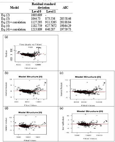
relatively big. Fit statistics improved significantly across equations. Decreased values of standard deviation and AIC were regarded as improved fit statistics. It is revealed that Eq. (4) with correlation structure error added is the best model among the proposed models.
It can be seen in the Fig. 1. that the residual plots against the fitted values become better across the models. Adding correlation factor in the model was significantly improved the fit.
Table 2. Fit statistics for equation (2)–(4)
Residual standard deviation Model
Level 0 Level 1
AIC
Eq. (2) 1003.689 -
Eq. (3) 1044.73 873.556 20558.46
Eq. (3) + correlation 1127.293 911.3265 20188.84
Eq. (4) 1182.759 627.7672 19864.29
Eq. (4) + correlation 1213.809 640.287 19759.73
(a)
(b) (c)
(d) (e)
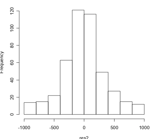
To further evaluate the results we predict production rate using validation dataset and calculate the standard deviation of the residuals. As the last model is the best, we validate this model only. The standard deviation residual of validation dataset is 364.0966. The histogram of this residual (Fig. 2) showed that it distributed normally.
Histogram of res2
res2
F
req
ue
n
c
y
-1000 -500 0 500 1000
0
20
4
0
6
0
80
1
00
120
Figure 2. The histogram of residuals validation dataset using Eq. 4 with adding correlation factor.
4. CONCLUSION
In this paper, we proposed the random effect regression in model for production rate by taking location as a random variable. The empirical study results indicate that using mixed effect and adding correlation structure improved the fit.
REFERENCES
Harville, D.A., 1977. Maximum likelihood approaches to variance component estimation and to related problems. J. Amer.Statist.Assoc. 72(358), 320-340.
Laird, N.M., Ware, J.H., 1982. Random-effects models for longitudinal data. Biometrics 38, 963-974.
Pinheiro, J. C., Bates, D. M., 2000. Mixed-effects models in S and S-PLUS. Statistics and Computing. Springer, New York.
Sohn, S.Y., 2002. Robust design of server capability in M/M/1 queues with both partly random arrival and service rates. Computers and Operation Research 29, 433-440.
Sohn, S.Y., 2006. Random effects logistic regression model for ranking efficiency in data envelopment analysis. The Journal of Operational Research Society 57 (11), 1289-1299.