A.Description of the Data
In this case, the writer divided the data of the students scores taken from on the
students’ English writing scores between those who taught using authentic materials
and who taught using non-authentic materials of Eighth Grade Students of MTs
Islamiyah Palangka Raya.
1. Scores of the students’ pre-test of experimental and control classes
a. Scores of the students’ pre-test of experimental class
Based on the test, the writer constructed the result are analyzed in following
ways:
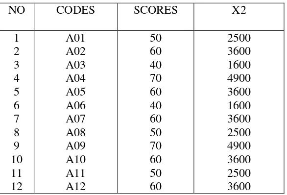
Table 4.1
Students’ Scores of Pre-Test of Experimental Class
13
From the data above it is known highest score is 70, and the lowest score is
40.
The writer got the data from the result of test. It can be known:
High score: 70, low score: 40
Range of score: R = H – L + 1
= 70 – 40 + 1
= 31
Furthermore, the writer arranged the data of the students’ scores as can be
seen in the following table:
Table 4.2
The Distribution of Frequency of the students’ scores of pre-test of
Total 22 100 Note: p = f / n × 100%
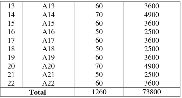
From the table above, it can be explained that on number 1 (one) there are 4
(four) students or about (18.18%) who obtained score 70. On number 2 (two) there
are 10 (ten) students or about (45.46%) who obtained score 60. On number 3
(three) there are 6 (six) students or about (27.27%) who obtained score 50. On
number 4 (four) there are 2 (two) students or about (9.09%) who obtained score
40.
From the distribution of frequency above, the writer constructed the
histogram as follow:
Figure 4.1 Histogram of Frequency Distribution of Students’ Scores of Pre
-Test of Experimental Class 0
2 4 6 8 10 12
These are calculation of mean, median and modus can be seen at the
following table:
1) Mean
The description and calculation of mean are presented in the following
table:
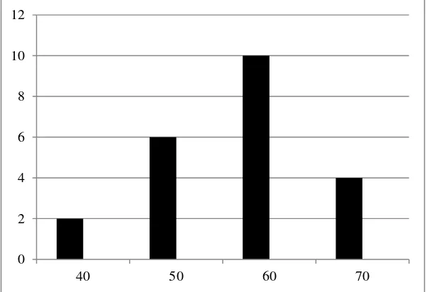
Table 4.3
The Calculation of Mean
NO X (SCORES) F fX
1 2 3 4
70 60 50 40
4 10
6 2
280 600 300 80 Total Ʃf = 22 ƩfX = 1260
From the data above, it is known:
∑fX Mx = N
1260 = 22
= 57.27
From the result of calculation above, it can be known that the mean score
2) Median
The description and calculation of median are presented as follows:
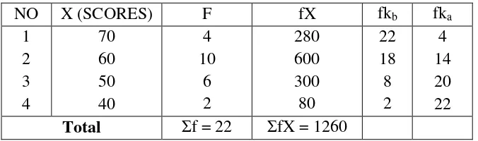
Table 4.4
The Calculation of Median
NO X (SCORES) F fX fkb fka
From the data above, it is known:
= 59.5 + 0,3
= 59.8
3) Modus
The description and calculation of modus are presented in the following
table:
Table 4.5
The Calculation of Modus
NO SCORES (X) F
1 2 3 4
70 60 50 40
4 10
6 2
Total Ʃf = 22
From the data above, it is known that Modus is 60. It is known from score
which has highest frequency.
b. Scores of the students’ pre-test of control class
Based on the test, the writer constructed the result are analyzed in the
following ways:
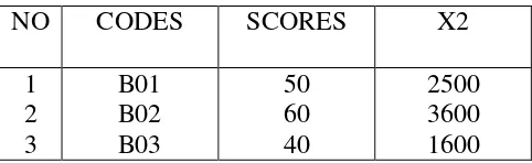
Table 4.6
Students’ Scores of pre-test of Control Class
NO CODES SCORES X2
1 2 3
B01 B02 B03
50 60 40
4
From the data above it is known highest score is 70, and the lowest score is
40.
The writer got the data from the result of test. It can be known:
High score: 70
Low score: 40
Range of score: R = H – L + 1
= 70 – 40 + 1
= 31
Furthermore, the writer arranged the data of the students’ scores as can be
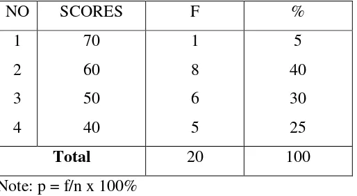
Table 4.7
The Distribution of Frequency of the students’ scores of pre-test of control
class
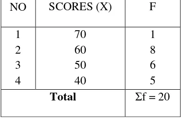
NO SCORES F %
1
2
3
4
70
60
50
40
1
8
6
5
5
40
30
25
Total 20 100
Note: p = f/n x 100%
From the table above, it can be explained that on number 1 (one) there is 1
(one) students or about (5%) who obtained score 70. On number 2 (two) there are
8 (eight) students or about (40%) who obtained score 60. On number 3 (three)
there are 6 (six) students or about (30%) who obtained score 50. On number 4
From the distribution of frequency above, the writer constructed the
histogram as follow:
Figure 4.2 Histogram of Frequency Distribution of Students’ Scores of Pre -test of Control Class
These are calculation of mean, median and modus can be seen at the
following table:
1) Mean
The description and calculation of mean are presented in the following
table:
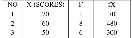
Table 4.8
The Calculation of Mean
NO X (SCORES) F fX
1 2 3
70 60 50
1 8 6
70 480 300 0
1 2 3 4 5 6 7 8 9
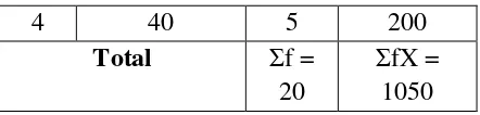
4 40 5 200
Total Ʃf =
20
ƩfX = 1050
From the data above, it is known:
∑fX
From the result of calculation above, it can be known that the mean score
which have been obtained 52.5
2) Median
The description and calculation of median are presented as follows:
Table 4.9
The Calculation of Median
NO X (SCORES) f fX fkb fka
From the data above, it is known:
Mdn = 60
l = 59.5
fkb = 11
fi = 8
yields:
½N – fkb Median = l +
fi
10 – 11 = 59.5 +
8
= 59.5 − 0.125
= 59.375
3) Modus
The description and calculation of modus are presented in the following
table:
Table 4.10
The Calculation of Modus
NO SCORES (X) F
1 2 3 4
70 60 50 40
1 8 6 5
From the data above, it is known that Modus is 60. It is known from score
which has highest frequency.
2. Scores of the students’ post-test of experimental and control class a. Scores of the students’ post-test of experimental class
Based on the test, the writer constructed the result are analyzed in following
ways:
Table 4.11
Students’ Scores of Post-Test of Experimental Class
Total 1550 110500
From the data above it is known that highest score is 80, and the lowest
score is 60.
The writer got the data from the result of test. It can be known:
High score: 80, low score: 60
Range of score: R = H – L + 1
= 80 – 60 + 1
= 21
Furthermore, the writer arranged the data of the students scores as can be
seen in the following table:
Table 4.12
The Distribution of Frequency of the students’ score of post-test of
Experimental Class
NO SCORES F %
1
2
3
80
70
60
7
9
6
31.82
40.91
27.27
Total 22 100
Note: p = f / n × 100%
From the table above, it can be explained that on number 1 (one) there are 7
there are 9 (nine) students or about (40.91%) who obtained score 70. On number 3
(three) there are 6 (six) students or about (27.27%) who obtained score 60.
From the distribution of frequency above, the writer constructed the
histogram as follow:
Figure 4.3 Histogram of Frequency Distribution of Students’ Scores of
post-test of Experimental Class 27,27
40,91
31,82
0 1 2 3 4 5 6 7 8 9 10
These are calculation of mean, median and modus can be seen at the
following table:
1) Mean
The description and calculation of mean are presented in the following
table:
Table 4.13
The Calculation of Mean
NO X (SCORES) F fX
1 2 3
80 70 60
7 9 6
560 630 360 Total Ʃf = 22 ƩfX = 1550
From the data above, it is known:
∑fX Mx = N
1550 = 22
= 70.45
From the result of calculation above, it can be known that the mean score
2) Median
The description and calculation of median are presented as follows:
Table 4.14
The Calculation of Median
NO X (SCORES) F fX fkb fka
1 2 3
80 70 60
7 9 6
560 630 360
22 15 6
7 16 22 Total Ʃf = 22 ƩfX = 1550
From the data above, it is known:
N = 22, ½ N = 11
Mdn = 70
l = 69.5
fkb = 6
fi = 9
yields:
½N – fkb Median = l +
fi
11 – 6 = 69.5 +
9
= 70.056
3) Modus
The description and calculation of modus are presented in the following
table:
Table 4.15
The Calculation of Modus
NO SCORES (X) F
From the data above, it is known that Modus is 70. It is known from score
which has highest frequency.
b. Scores of the students’ post-test of control class
Based on the test, the writer constructed the result are analyzed in the
following ways:
Table 4.16
Students’ Scores of post-test of Control Class
7
From the data above it is known highest score is 70, and the lowest score is
50.
The writer got the data from the result of test. It can be known:
High score: 70
Low score: 50
Range of score: R = H – L + 1
= 70 – 50 + 1
Furthermore, the writer arranged the data of the students’ scores as can be
seen in the following table:
Table 4.17
The Distribution of Frequency of the students’ scores of Control Class
NO SCORES F %
1
2
3
70
60
50
5
8
7
25
40
35
Total 20 100
Note: p = f/n x 100%
From the table above, it can be explained that on number 1 (one) there are 5
(five) students or about (25%) who obtained score 70. On number 2 (two) there are
8 (eight) students or about (40) who obtained score 60. On number 3 (three) there
are 7 (seven) students or about (35%) who obtained score 50.
From the distribution of frequency above, the writer constructed the
Figure 4.4 Histogram of Frequency Distribution of Students’ Scores of
post-test of Control Class
These are calculation of mean, median and modus can be seen at the
following table:
1) Mean
The description and calculation of mean are presented in the following table:
Table 4.18
The Calculation of Mean
NO X (SCORES) F fX
1 2 3
70 60 50
5 8 7
350 480 350 Total Ʃf = 20 ƩfX = 1180 35
40
25
0 1 2 3 4 5 6 7 8 9
From the data above, it is known:
∑fX Mx =
N
1180 =
20
= 59
From the result of calculation above, it can be known that the mean score
which have been obtained 59
2) Median
The description and calculation of median are presented as follows:
Table 4.19
The Calculation of Median
NO X (SCORES) f fX fkb fka
1 2 3
70 60 50
5 8 7
350 480 350
20 15 7
5 13 20 Total Ʃf = 20 ƩfX = 1180
From the data above, it is known:
N = 20, ½ N = 10
Mdn = 60
l = 59.5
fi = 8
yields:
½N – fkb Median = l +
fi
10 – 7 = 59.5 +
8
= 59.5 + 0.375
= 59.875
3) Modus
The description and calculation of modus are presented in the following
table:
Table 4.20
The Calculation of Modus
NO SCORES (X) F
1 2 3
70 60 50
5 8 7 Total Ʃf = 20
From the data above, it is known that Modus is 60. It is known from score
B.Result of the Data Analysis
1. Deviation standard of the students’ post-test of experimental class of eighth
grade students of MTs Islamiyah Palangka Raya.
The calculation of deviation standard is presented in the following table:
Table 4.21
The Calculation of Deviation Standard of Experimental Class
Scores (X) f fX X x2 fx2
80 7 560 9.55 91.2025 638.4175
70 9 630 -0.45 0.2025 1.8225
60 6 360 -10.45 109.2025 655.215
Total Ʃf = 22 ƩfX = 1550 Ʃfx2 = 1295.455
To know the deviation standard where:
SD = √ ∑fx2 N
SD = √ 1550
22
2.Deviation standard of the students’ post-test of Control Class of eighth
grade students of MTs Islamiyah Palangka Raya.
The calculation of deviation standard is presented in the following table:
Table 4.22
The Calculation of Deviation Standard of Control Class
Scores (X) F fX X x2 fx2
70 5 350 11 121 605
60 8 480 1 1 8
50 7 350 -9 81 567
Total Ʃf = 20 ƩfX = 1180 Ʃfx2 = 1180
To know the deviation standard where:
SD = √ ∑fx2 N
SD = √ 1180
20
SD = 7.681
3. The Calculation of T-test
Table 4.23
The Calculation of T-test
NO
Students’ scores before taught using authentic
materials (X)
Students’ scores after taught using non-authentic materials
(Y)
D D2
1 50 70 -20 400
2 60 70 -10 100
4 70 80 -10 100
5 60 70 -10 100
6 40 60 -20 400
7 60 70 -10 100
8 50 60 -10 100
9 70 80 -10 100
10 60 70 -10 100
11 50 60 -10 100
12 60 80 -20 400
13 60 70 -10 100
14 70 80 -10 100
15 60 70 -10 100
16 50 60 -10 100
17 60 80 -20 400
18 50 60 -10 100
19 60 70 -10 100
20 70 80 -10 100
21 50 70 -20 400
22 60 80 -20 400
-290 4300
To know mean of difference, the writer used formula:
MD = ƩD N
MD = -290 22
MD = -13.18
To know SDD (Standard of Deviation of difference between score variable I
and Score variable II), the writer used formula:
SDD= √ ∑D2 – ∑D 2
N N
SDD = √4300 – -290 2
22 22
SDD = √ 195.45454545 – 173.765124
SDD = 4.6571902957
To Calculate SEMD (Standard Error of Mean of Difference), the writer used
formula:
SEMD = SDD
√N-1
SEMD = 4.6571902957
√22-1
SEMD = 4.6571902957
4.5825756949
SEMD = 1.0162822408
To know to (tobserved), the writer used formula:
t0 = MD SEMD
t0 = -13.18 1.0162822408
t0 = -12.969
To know df (degree of freedom), the writer used formula:
df = Nx + Ny – 2
= 22 + 22 – 2
= 42
With the criteria:
If ttest (t0) > ttable, Ha is accepted and Ho is rejected
If ttest (t0) < ttable, Ha is rejected and Ho is accepted
Based on the data obtained, the result showed that the mean of students’
English writing scores of who taught using authentic materials was 70.45, while
the mean of students’ English writing scores of who taught using non-authentic
material was 59. From both means, there was different value that was 11.45. It
meant there is different result of them in writing recount paragraphs. Furthermore,
the writer arranged the Mean Scores of students’ scores pre-test and students’
scores post-test of both classes as can be seen in the following table:
Table 4.24
Mean Scores of Students’ Scores Pre-test and Post-test of Experimental and Control Classes
Mean Scores of Pre-test Mean Scores of Post-test Different Values Experiment Control Experiment Control Pre-test Post-test
Based on the calculation above, it can be known the value from the result of
calculation (tobserved) was -12,969. Then, it is consulted with ttable (tt) which db or df
= (N1 + N2 ) – 2 was (22 + 22) – 2 = 42. Significant standard 5% ttable (tt) = 2.02
and significant standard 1% ttable (tt) = 2.71. So, 2.02 < 12.969 > 2.71. It can be said that since the value of tobserved (-12.969) was higher than ttable in the 5% (2.02)
and 1% (2.71) level of significance, it could be interpreted that Ha stating that
there is a significant difference between who taught using authentic materials and
who taught using non-authentic material of eighth grade students of MTs
Islamiyah of Palangka Raya was accepted and Ho stating that there is no
significant difference between who taught using authentic materials and who
taught using non-authentic material of eighth grade students of MTs Islamiyah of
Palangka Raya was rejected. It meant that there is a significant difference between
Meanwhile, the writer also applied SPSS program to calculate t-test:
Table 4.25
The Calculation of the Result T-test using SPSS 16
Paired Samples Test Paired Differences
T df Sig.
(2-tailed) Mean
Std. Devia
tion
Std. Error Mean
95% Confidence Interval of the
Difference
Lower Upper
Pair 1
Pre-test Scores of Experimental Class - Post-test Scores of Experimental Class
-13.182 4.767 1.016 -15.296 -11.068 -12.969 42 .000
The result of the t-test using SPSS also supported the interpretation above
that was found the tobserved (-12.969). Significant standard 5% ttable (tt) = 2.02 and
significant standard 1% ttable (tt) = 2.71. So, 2.02 < 12.969 > 2.71. It can be said that since the value of tobserved (-12.969) was higher than ttable in the 5% (2.02) and
1% (2.71) level of significance, it could be interpreted that Ha stating that there is
a significant difference between who taught using authentic materials and who
taught using non-authentic material of eighth grade students of MTs Islamiyah of
Palangka Raya was accepted and Ho stating that there is no significant difference
material of eighth grade students of MTs Islamiyah of Palangka Raya was
rejected. It meant that there is a significant difference between who taught using