View of AN EXPERIMENTAL STUDY ON BANK FORECASTING USING REGRESSION DYNAMIC LINIER MODEL

AN EXPERIMENTAL STUDY ON BANK

FORECASTING USING REGRESSION DYNAMIC

LINIER MODEL

Wiwik Anggraeni1

Danang Febrian2

e-mail : anggraeni@gmail.com, danang_febrian@yahoo.co.id

Diterima : 20 Mei 2011/ Disetujui : 24 Juni 2011

ABSTRACT

Nowadays, forecasting is developed more rapidly because of more systematicaly decision making process in companies. One of the good forecasting characteristics is accuration, that is obtaining error as small as possible. Many current forecasting methods use large historical data for obtaining minimal error. Besides, they do not pay attention to the influenced factors. In this final project, one of the forecasting methods will be proposed. This method is called Regression Dynamic Linear Model (RDLM). This method is an expansion from Dynamic Linear Model (DLM) method, which model a data based on variables that influence it. In RDLM, variables that influence a data is called regression variables. If a data has more than one regression variables, then there will be so many RDLM candidate models. This will make things difficult to determine the most optimal model. Because of that, one of the Bayesian Model Averaging (BMA) methods will be applied in order to determine the most optimal model from a set of RDLM candidate models. This method is called Akaike Information Criteria (AIC). Using this AIC method, model choosing process will be easier, and the optimal RDLM model can be used to forecast the data. BMA-Akaike Information Criteria (AIC) method is able to determine RDLM models optimally. The optimal RDLM model has high accuracy for forecasting. That can be concluded from the error estimation results, that MAPE value is 0.62897% and U value is 0.20262.

Keyword : Forecasting, Regression variables, RDLM, BMA, AIC

1 . Information System Department, Institut Teknologi Sepuluh Nopember

Kampus Keputih, Sukolilo, Surabaya 60111, Indonesia

2 . Information System Department, Institut Teknologi Sepuluh Nopember

INTRODUCTION

Nowadays, forecasting has developed more rapidly because of the more systematically decision making in a organization or company. One of the good forecasting characteristic is from accuration, and should get error that is as minimal as possible. Usually, forecasting just estimates based on historical data only without considering external factors that might influence the data. Because of that, in this paper will be proposed a method that takes all external factors into consideration, this method is called Regression Dynamic Linear Models (RDLM), with Bayesian Model Averaging (BMA) applied in order to choose the most optimal model. By using this method, the forecast results will have high accuracy. (Mubwandarikwa et al., 2005).

The Method

There are four steps to forecast a data using RDLM method, i.e. : forming candidate models, choosing optimal model, forecasting using optimal model, and measuring accuracy of optimal model.

Dynamic Linear Models (DLM)

Dynamic Linear Model is an extension of state-space modeling on prediction and dynamic system control (Aplevich, 1999). State-space model of time series contains data generating process with state (usually shown by vector of parameter) that can change over time. This state is only observed indirectly, as far as values of time series that are obtained as function of state in correspond period. DLM base model at all time t is described by evolution / system and observation equation. The equation forms are as follow :

o Observation equation :

, o System equation :

, o Initial information :

>

0 0

@

0 ~ N m ,C

T (3)

DLM can be explained alternatively with 4 sets as follow :

Where at time t, :

o T_t is state vector at time t.

o F_t is known regression variable vector.

o v_t is observation noise that has Gaussian distribution with zero mean and

known variance V_t, where it represents estimation and error trial of changing

observation of Y_t.

o G_t is state evolution matrix, it describes deterministic mapping of state vector between time t – 1 and t.

o Z_tis evolution noise that has Gaussian distribution with zero mean and variance matrix Wt, where it represents changing in state vector.

Regression Dynamic Linear Models (RDLM)

Regression Dynamic Linear Model (RDLM) is an extension of DLM, which RDLM considers regression variables (regressor) in modeling process. For example, for time series data that has regressors X1, X2, then it will have several possible models, that are M1( ,X1), M2( ,X2) and M3( ,X1,X2). For time t, t = 1,2,… Regression Dynamic Linear Model (RDLM), ,(j = 1,2,...,k), represents a base time series model with 4 observations, which can be identified by 4 sets, where :

o F_j (X1,...,Xp)_j is regression vector (1 x p), Xij is ith variable regression

(i =1,2,...,p) which for X₁ has value of 1.

o G_j is system evolution matrix (p x p) with the value of Gj I(n) identity

matrix.

o V_j is observation variance of .

o is system evolution variance matrix (p x p) which is estimated using discount factors, for ith _{time :}

t

jt C

W

G G

1

(5)

Discount factors are determined by checking off model to determine the optimal

values. Optimal value for trend component G_T 0.9, seasonality G_S 0.95 ,

RDLM Sequential Updating

Estimation of state variables (T ) can not be done directly at all times, but by using

information from data which update from time t-1 to t is performed using Kalman Filter. For further information, see West and Harrison (1997).

Take as example D_t describes all information from past times until time t and Y_tis

data at time t.

Equation (2) and (6) have Gaussian distribution, so linear combinations of both of them can be formed and produce prior distribution that is :

)

Then from equation (1) and (7), forecast distribution can be obtained, that is :

)

From forecast distribution at equation (8), forecast result for Y_t can be obtained using :

By using Kalman Filter, posterior distribution can be obtained :

)

All the steps above solve recursive update of RDLM and can be summaried as following :

1. determining model by choosing [F,G,V,W]_t.

2. setting initial values of m₀,c₀.

4. observing y_t1 and updating using equation (10). 5. back to (c), then substituting t+1 with t.

Bayesian Model Averaging of RDLM

In RDLM method, there are many candidate models. For determining the most optimal model, one of BMA method is used, that is Akaike Information Criteria (AIC).

Akaike Information Criteria (AIC)

Akaike Information Criteria (AIC) by Akaike (1974) originates from maximum (log-)likelihood estimate (MLE) from error variance of Gaussian Linear regression model. Maximum (log-) likelihood model can be used to estimate parameter value in classic linier regression model. AIC suggests that from a class of candidate models, choose model that minimize :

p Lj

AIC 2ln 2 (11)

Where for jth _{model :}

o Ljis likelihood.

o p is number of parameters in model.

This method chooses model that gives best estimates asymptotically (Akaike, 1974) in explanation of Kullback-Leibler. Akaike weight can be estimated by defining:

) min(AIC AIC_j

j

' (12)

where minAIC is the smallest value of AIC in a set of models. Likelihood Ljfrom

every model M_j(j) conditional on data and set of models. Then Akaike weight

j

w can be estimated using equation :

¦

'

Error Estimation

For knowing the accuration of forecasting model, it can be seen from error estimation result. According to Makridakis et al., 1997, several methods in forecast error estimation that can be used are as following :

o Mean Absolute Percentage Error (MAPE)

MAPE is differences between real data and forecast result that is divided with forecast result then is absoluted and the result is on percent value. A model has excellent performance if MAPE value lies under 10%, and good performance if MAPE value lies between 10% and 20% (Zainun dan Majid, 2003).

¦

t

o Theil’s U statistic

U statistic is performance comparation between a forecasting model with naïve forecasting, that predicts future value is equivalent with real value one time before. Comparation takes correspond ratio with RMSE (root mean squared errors), that is square root of average squared differences between prediction and observation. As the main rule, forecasting method that has Theil’s U value larger than 1 is not effective.

where for all methods,

Y = data, Yˆ= forecasting result.

Implementation and Analysis

Several trial test that have been done are choosing optimal model, forecasting optimal model, testing AIC performance and comparing DLM with RDLM.

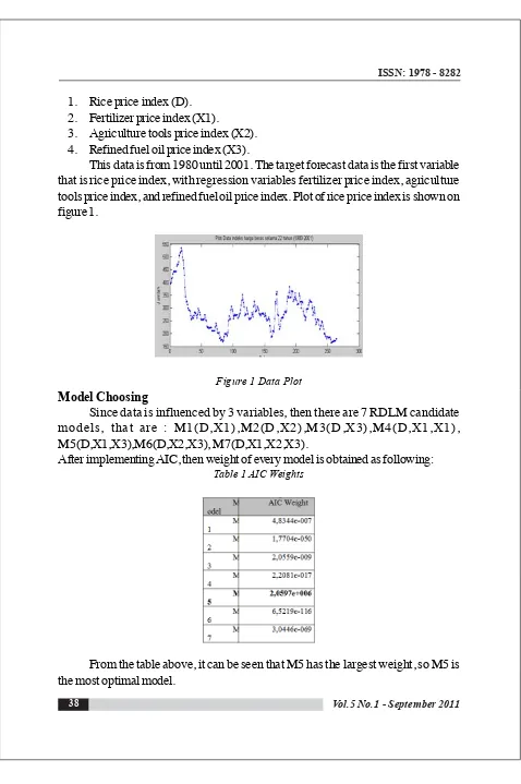
1. Rice price index (D). 2. Fertilizer price index (X1).

3. Agriculture tools price index (X2). 4. Refined fuel oil price index (X3).

This data is from 1980 until 2001. The target forecast data is the first variable that is rice price index, with regression variables fertilizer price index, agriculture tools price index, and refined fuel oil price index. Plot of rice price index is shown on figure 1.

Figure 1 Data Plot Model Choosing

Since data is influenced by 3 variables, then there are 7 RDLM candidate models, that are : M1(D,X1),M2(D,X2),M3(D,X3),M4(D,X1,X1), M5(D,X1,X3),M6(D,X2,X3), M7(D,X1,X2,X3).

After implementing AIC, then weight of every model is obtained as following:

Table 1 AIC Weights

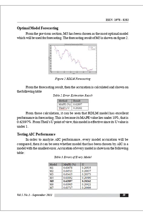
Optimal Model Forecasting

From the previous section, M5 has been chosen as the most optimal model which will be used for forecasting. The forecasting result of M5 is shown on figure 2.

Figure 2 RDLM Forecasting

From the forecasting result, then the accuration is calculated and shown on the following table

Table 2 Error Estimation Result

From those calculation, it can be seen that RDLM model has excellent performance in forecasting. This is because its MAPE value lies under 10%, that is 0.62897%. From Theil’s U point of view, this model is effective since its U value is under 1.

Testing AIC Performance

In order to analyze AIC performance, every model accuration will be compared, then it can be seen whether model that has been chosen by AIC is a model with the smallest error. Accuration of every model is shown on the following table :

It can be seen from the table above that M5 has the smallest error, so it can be concluded that AIC method works well in choosing model.

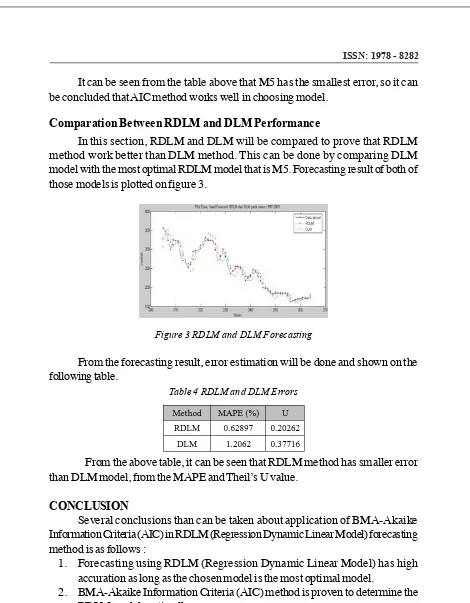
Comparation Between RDLM and DLM Performance

In this section, RDLM and DLM will be compared to prove that RDLM method work better than DLM method. This can be done by comparing DLM model with the most optimal RDLM model that is M5. Forecasting result of both of those models is plotted on figure 3.

Figure 3 RDLM and DLM Forecasting

From the forecasting result, error estimation will be done and shown on the following table.

Table 4 RDLM and DLM Errors

From the above table, it can be seen that RDLM method has smaller error than DLM model, from the MAPE and Theil’s U value.

CONCLUSION

Several conclusions than can be taken about application of BMA-Akaike Information Criteria (AIC) in RDLM (Regression Dynamic Linear Model) forecasting method is as follows :

1. Forecasting using RDLM (Regression Dynamic Linear Model) has high accuration as long as the chosen model is the most optimal model.

3. Forecasting using RDLM method has better result than normal DLM method as long as the RDLM model is the most optimal model.

4. Using rice price index data on 1997 – 2001, RDLM method works 48% better than DLM method judging from MAPE value, and 46% better judging from Theil’s U value.

DAFTAR PUSTAKA

1. Akaike, H. (1974), A new look at the Statistical model identication. IEEE Trans. Auto. Control, 19, 716-723.

2. Aplevich, J., (1999). The Essentials of Linear State-Space Systems. J. Wiley and Sons.

3. Grewal, M. S., Andrews, A. P., (2001). Kalman Filtering: Theory and Practice Using MATLAB (2nd ed.). J. Wiley and Sons.

4. Harvey, A., (1994). Forecasting, Structural Time-series Models and the Kalman Filter. Cambridge University Press.

5. Mubwandarikwa, E., Faria A.E. (2006) The Geometric Combination of Forecasting Models Department of Statistics, Faculty of Mathematics and Computing, The Open University.

6. Mubwandarikwa, E., Garthwaite, P.H., dan Faria, A.E., (2005). Bayesian Model Averaging of Dynamic Linear Models. Department of Statistics, Faculty of Mathematics and Computing, The Open University.

7. Turkheimer, E., Hinz, R. and Cunningham, V., (2003), On the undesirability among kinetic models: from model selection to model averaging. Journal of Cerebral Blood Flow & Metabolism, 23, 490-498.

8. Verrall R. J. (1983). Forecasting The Bayesian The City University, London 9. West , Mike. (1997). Bayesian Forecasting, Institute of Statistics & Decision

Sciences Duke University.

10. World Primary Commodity Prices.(2002). Diambil pada tanggal 23 Mei 2008 dari http://www.economicswebinstitute.org.

11. Yelland, Phillip M. & Lee, Eunice. (2003), Forecasting Product Sales with Dynamic Linear Mixture Models. Sun Microsystem.