Oliver Keszocze
Robert Wille
Rolf Drechsler
Exact Design
of Digital
Oliver Keszocze • Robert Wille • Rolf Drechsler
Exact Design of Digital
Microfluidic Biochips
University of Bremen and DFKI GmbH Bremen, Germany
Rolf Drechsler
University of Bremen and DFKI GmbH Bremen, Germany
Johannes Kepler University Linz Linz, Austria
ISBN 978-3-319-90935-6 ISBN 978-3-319-90936-3 (eBook) https://doi.org/10.1007/978-3-319-90936-3
Library of Congress Control Number: 2018942500
© Springer International Publishing AG, part of Springer Nature 2019
This work is subject to copyright. All rights are reserved by the Publisher, whether the whole or part of the material is concerned, specifically the rights of translation, reprinting, reuse of illustrations, recitation, broadcasting, reproduction on microfilms or in any other physical way, and transmission or information storage and retrieval, electronic adaptation, computer software, or by similar or dissimilar methodology now known or hereafter developed.
The use of general descriptive names, registered names, trademarks, service marks, etc. in this publication does not imply, even in the absence of a specific statement, that such names are exempt from the relevant protective laws and regulations and therefore free for general use.
The publisher, the authors and the editors are safe to assume that the advice and information in this book are believed to be true and accurate at the date of publication. Neither the publisher nor the authors or the editors give a warranty, express or implied, with respect to the material contained herein or for any errors or omissions that may have been made. The publisher remains neutral with regard to jurisdictional claims in published maps and institutional affiliations.
Printed on acid-free paper
This Springer imprint is published by the registered company Springer International Publishing AG part of Springer Nature.
Preface
Many biological or medical experiments today are conducted manually by highly trained experts. Usually, a large laboratory requiring a lot of equipment is needed as well. This makes the whole process expensive and does not allow for very high throughput. This led to the development of automated laboratory equipment such as automated robots. These devices already allow for a high level of automation and integration. Unfortunately, laboratory robots are usually bulky (and expensive) and also use rather large amounts of liquids, which may be very expensive on their own. To further reduce the size of laboratory devices, researchers investigated how to manipulate liquids at a nanoliter or even picoliter volume scale. This led to the development of microfluidic biochips, also known as lab-on-a-chip. The technical capabilities of microfluidic devices have been widely illustrated in the literature. An essential step for being able to actually make use ofDigital Microfluidic Biochips (DMFBs) is to properly design (or synthesize) those. This process includes to take a medical or biological assay description, a biochip geometry, and further constraints and determine a precise execution scheme for running the assay on the biochip. As biochips grow in size and more complex assays are to be conducted, manual design of these devices is often not feasible anymore. Moreover, manual designs are often far from being optimal. Instead, high-quality design methodologies are required which relieve the design burden of manual optimizations of assays, time-consuming chip designs, as well as costly testing and maintenance procedures.
This book presents exact, that is minimal, solutions to individual steps in the design process as well as to a one-pass approach that combines all design steps in a single step. The presented methods are easily adaptable to future needs. In addition to the minimal methods, heuristic approaches are provided and the complexity classes of (some of) the design problems are determined.
By this, the book summarizes the results of several years of intensive research at the University of Bremen, Germany, the DFKI GmbH Bremen, Germany, and the Johannes Kepler University Linz, Austria. This included several collaborations— most importantly with the group of Prof. Krishnendu Chakrabarty from the Duke University, USA, and the group of Prof. Tsung-Yi Ho from the National Tsing Hua University, Taiwan. We would like to sincerely thank both colleagues for
the very inspiring and fruitful joint work. Besides that, we are thankful to the coauthors of corresponding research papers which formed the basis of this book, including (in alphabetical order) Alexander Kroker, Andre Pols, Andreas Grimmer, Jannis Stoppe, Kevin Leonard Schneider, Maximilian Luenert, Mohamed Ibrahim, Tobias Boehnisch, and Zipeng Li. Furthermore, many thanks go to our research groups in Bremen and Linz for providing us with a comfortable and inspirational environment from which some authors benefit until today. Finally, we would like to thank Springer and, in particular, Charles “Chuck” Glaser for making this book possible.
Bremen, Germany Oliver Keszocze
Linz, Austria Robert Wille
Bremen, Germany Rolf Drechsler
Contents
1 Introduction . . . 1
2 Background. . . 11
2.1 Microfluidic Biochips. . . 11
2.1.1 Microfluidic Operations. . . 11
2.1.2 Fluidic Constraints. . . 12
2.2 Discrete DMFB Model. . . 14
2.2.1 Geometry of the Biochip. . . 15
2.2.2 Droplet Movement. . . 16
2.2.3 Electrode Actuation. . . 17
2.3 Reasoning Engines . . . 19
2.3.1 Boolean Satisfiability. . . 20
2.3.2 Satisfiability Modulo Theories. . . 20
2.3.3 Integer Linear Programming. . . 21
3 Routing. . . 23
3.1 Problem Formulation. . . 23
3.2 Complexity of Routing. . . 23
3.3 Heuristic Approaches. . . 28
3.4 Proposed Solution. . . 29
3.4.1 SAT Variables. . . 30
3.4.2 SAT Constraints. . . 31
3.5 Experimental Results. . . 34
3.6 Summary. . . 37
4 Pin Assignment. . . 39
4.1 Problem Formulation. . . 39
4.2 Complexity of Pin Assignment . . . 40
4.2.1 Reduction from Pin Assignment to Graph Coloring. . . 41
4.2.2 Reduction from Graph Coloring to Pin Assignment. . . 42
4.3 Related Work . . . 44
4.4 Proposed Solutions. . . 45
4.4.1 Heuristic Approach. . . 45
4.4.2 Exact Solution . . . 47
4.5 Experimental Results. . . 48
4.5.1 Evaluation of the Pin Assignment. . . 49
4.5.2 Optimizing the Pin Assignment. . . 51
4.6 Summary. . . 53
5 Pin-Aware Routing and Extensions. . . 55
5.1 Pin-Aware Routing . . . 55
5.1.1 SMT Formulation. . . 55
5.1.2 Related Work. . . 57
5.1.3 Use Cases. . . 57
5.2 Routing with Timing Information . . . 60
5.3 Aging-Aware Routing. . . 63
5.4 Routing with Different Cell Forms. . . 66
5.4.1 Problem Formulation. . . 67
5.4.2 Transformation of Routing Problems. . . 68
5.4.3 SMT Formulation. . . 68
5.4.4 Experimental Results. . . 69
5.5 Routing for Micro-Electrode-Dot-Array Biochips. . . 70
5.5.1 Motivation and Background. . . 70
5.5.2 MEDA Model and Problem Formulation. . . 72
5.5.3 Related Work. . . 74
5.5.4 Proposed Exact Routing Approach. . . 75
5.5.5 Experimental Results. . . 81
5.6 Summary. . . 84
6 One-Pass Design. . . 87
6.1 The Design Gap Problem . . . 87
6.2 Proposed Solutions. . . 88
6.2.1 Heuristic One-Pass Design. . . 88
6.2.2 Exact One-Pass Design. . . 94
6.3 Experimental Results. . . 102
6.3.1 Considered Benchmarks. . . 102
6.3.2 Implementations. . . 102
6.3.3 Evaluation of the Solution Length. . . 103
6.3.4 Evaluating Iteration Schemes. . . 105
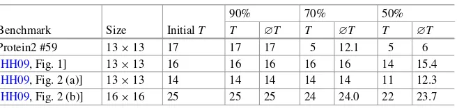
6.3.5 Trade-Off Between Grid Size and Time Steps . . . 106
6.4 Summary. . . 107
Contents ix
Appendix A BioGram: A Dedicated Grammar for DMFB Design. . . 111
Appendix B BioViz: An Interactive Visualization Tool for DMFB Design . . . 115
B.1 The Graphical User Interface. . . 116
B.2 Use Case: Interactive Routing . . . 119
B.2.1 Implementation. . . 120
B.2.2 Routing Algorithms. . . 120
B.2.3 Case Study. . . 121
Appendix C Notation. . . 123
References. . . 125
Introduction
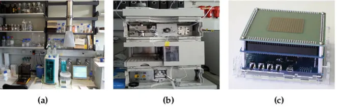
Today, many biological or medical experiments are conducted manually by highly trained experts. Usually, a large laboratory requiring a lot of equipment is needed as well (see Fig.1.1a which shows a typical laboratory setup). This makes the whole process expensive and does not allow for very high throughput. Furthermore, as human beings are no perfectly working robots, they are a source of errors, especially when many repetitive and monotonous steps are involved in a biological assay.
This led to the development of automated laboratory equipment such as the robots shown in Fig.1.1b. These devices already allow for a high level of automation and integration, even though in many cases they only physically imitate the steps a human being would perform. Despite already significantly easing laboratory work, this still leaves room for improvement since those laboratory robots are usually bulky (and expensive).
To further reduce the size of laboratory devices, researchers investigated how to manipulate liquids at a nanoliter or even picoliter volume scale. This led to the development ofmicrofluidic biochips(see Fig.1.1c), also known aslab-on-a-chip. These are devices that automatically manipulate small amounts of liquids in order to perform (a subset of) the same experiments previously conducted in a laboratory. In addition to simply saving liquids, which may be expensive or difficult to obtain, smaller volumes can also result in shorter experiment execution times. In general, a higher throughput and sensitivity may be achieved.
The capabilities of microfluidic devices has been widely illustrated in the literature. Early works successfully demonstrate the applicability of biochips for multiplexed real-timepolymerase chain reaction(PCR) [Liu+04] and colorimetric glucose assay for various bodily fluids [Sri+03]. In [Fai+07], different applications for biochips, such as massively parallel DNA analysis, real-time bio-molecular detection and recognition are presented. In [HZC10], protein crystallization for drug discovery and glucose measurement for blood serum are reported to have successfully been implemented. Another area where biochips are of interest is sample preparation [HLC12, Bha+17a, Bha+17b]. Using biochips, this tedious
© Springer International Publishing AG, part of Springer Nature 2019 O. Keszocze et al.,Exact Design of Digital Microfluidic Biochips,
https://doi.org/10.1007/978-3-319-90936-3_1
2 1 Introduction
Fig. 1.1 Development in equipment size. (a) Laboratory. (b) Robot. (c) Biochip
process can be automatized to a high degree. In [Sis+08], biochips capable of executing different types of assays are used for point-of-care diagnostics. As has been pointed out in [Ali+17], biochips may be the future of easily accessible health-care. One scenario is to conduct on-site tests for diseases in remote regions. Besides that, also applications, e.g., for bubble logic [CYK07,PG07] or stochastic computing [HGW17] have been considered.
Motivated by this, different kinds of biochips and corresponding derivatives have been introduced which rely on different technologies. For example, valve-based biochipsare composed of integrated microvalves [Hu+14,Mar+10], which are used to control the flow of liquids. Such biochips are made of materials such as glass, plastic, or polymers. Functionality, such as mixing liquids, is realized by fabricating corresponding channels at given positions. The microfluidic channels are used to transport the liquids to these positions. While, originally, such chips were rather static (similar to ASICs from conventional circuitry), in the meanwhile also more dynamic solutions have been proposed in terms ofProgrammable Microfluidic Devices(PMDs; similar to an FPGA from conventional circuitry [FM11,JBM10]). Figure 1.2 shows a valve-based biochip. While the chip itself is quite small in size, it still needs external hardware such as pressure sources. The overhead by the connectors to the chip itself is evident. The need for external hardware makes the operation of such a biochip “in the field” quite complicated.
Fig. 1.2 Physical realization of a flow-based biochip of the size of a dime [Whi06, Figure 1]
Fig. 1.3 Physical realization of a digital microfluidic biochip: zig-zag lined electrodes
lines but as zig-zag lines, resulting in “interleaved” electrodes (see Fig.1.3). Also this concept has been generalized so that eventually so-called Micro-Electrode-Dot-Arraybiochips (MEDA biochips, [Li+16,Che+11,WTF11]) resulted. Here, liquids are not controlled by single electrodes, but asea-of-micro-electrodesis employed to allow for different droplet sizes and shapes.
Besides that, many further biochip technologies exist and/or recently received attention including, e.g., paper-based biochips as proposed in [WLH16a,WLH16b] or pressure-driven biochips (employing, e.g., the concept of two-phase flow microfluidics) as proposed in [De +12,Don+15,Don+14,De +13] which eventually resulted in a concept known asNetworked Labs-on-Chips(NLoC, [De +12]).
4 1 Introduction
developed during the writing of this book. These devices can be manufactured in a very compact manner. The presented biochip is of dimension 11 cm×11 cm×6 cm and needs no further external equipment besides a common 12 V power supply. This is one major advantage of digital microfluidic biochips over flow-based biochips. No external pressure source or further equipment is required. Besides that, there also exist many successfully commercialized biochips such as Illumina’s NeoPrep system [Illumina]. According to a report released by Research and Markets in June 2013, the global biochip market will grow from 1.4 billion in 2013 to 5.7 billion by 2018 [Market13].
However, in order to utilize these prospects, a corresponding biochip has to be designed (or synthesized) so that indeed the desired experiment is executed and, additionally, all constraints, e.g., with respect to the completion time are satisfied. This process includes to take a medical or biological assay description, a biochip, and further constraints, such as the maximally allowed completion time of the experiment, and use this input to determine a precise execution scheme for running the assay on the biochip. For the different kind of biochip technologies, a significant amount of corresponding automatic design methods have been proposed (see, e.g., [CZ05,Wan+17,Gri+17b] for valve-based biochips, [SHL16,Gri+18b] for PMD, [WLH16a,WLH16b] for paper-based biochips, or [Gri+18a,Gri+17c] for NLoCs). In this book, we will mainly focus on the automatic design of DMFBs (although many methods proposed here can also be applied for other biochip technologies).
Here, the objective of synthesis is to realize an experiment on the layout of the given biochip and within an upper bound on the completion time. To this end, the following design questions need to be addressed:
• Which modules shall be used in order to realize an operation? (binding) • When (at what time steps) shall each operation be conducted? (scheduling) • Where (on which cells) shall each operation be conducted? (placement)
• Which paths shall the corresponding droplets take in order to reach their destinations? (routing)
• Which electrodes can be grouped together in order to allow for a simpler control logic? (pin assignment)
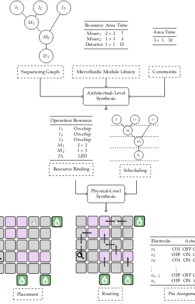
These five steps are conducted in a two-stage design flow composed of an architecture-level synthesis(binding and scheduling) and aphysical-level synthesis (placement, routing, and pin assignment) as illustrated in Fig.1.4.
The input of a design problem usually consists of the following three parts. Sequencing Graph The sequencing graph describes the experiment in terms of
operations and their interdependence. The sequencing graph implicitly defines the number of droplets and devices that are necessary. A sequencing graph is shown in the top left corner of Fig.1.4.
Sequencing Graph
I1 I2 I3
M1
M2
D1
Microfluidic Module Library Resource Area Time
Mixer1 2×2 7 Mixer2 1×3 4 Detector1×1 15
Constraints Area Time
5×5 50
Architectual-Level Synthesis
Operation Resource
I1 On-chip
I2 On-chip
I3 On-chip
M1 2×2
M2 1×3
D1 LED Resource Binding
I1 I2 I3 M1
M2 D1 Scheduling
Physical-Level Synthesis
Placement Routing Pin Assignment
Electrode Actuation
v1 ON OFF OFF . . .
v2 OFF ON OFF . . .
v3 ON ON OFF . . .
vn−1 OFF OFF OFF . . .
vn OFF ON ON . . .
Fig. 1.4 Design flow for digital microfluidic biochips
6 1 Introduction
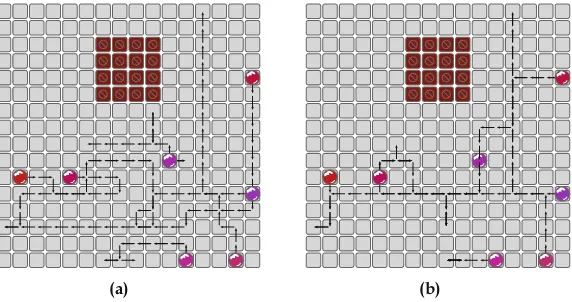
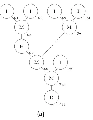
Fig. 1.5 (a) Sequencing graph and (b) module library for an experiment
A possible realization of the experiment as described in Fig.1.5is explained in the following example.
Example 1.1 Figure 1.6illustrates the realization of the experiment on a 5×5 biochip. The visualization is shown in Fig.1.6a while the precise timing information is shown in Fig.1.6b. In the first time step, the droplets 1,2,and 3 are dispensed. While the droplets 1 and 2 are mixed for 15 time steps in the lower mixer (indicated by the highlighted cells), droplet 3 is heated to its desired temperature for 13 time steps. The heated droplet 3 and the result of the mixing operation are then mixed for another 17 time steps. The resulting droplet is eventually analyzed by the detector in time steps 38–56. As can be seen, different fashions of modules are used for the mixing operation. The first mixer required 1×3 cells and 15 time steps, while the second one occupied a 2×2 cells over 17 time steps. Note that the time steps needed for the droplet movements are not explicitly listed in the table in Fig.1.6b.
As biochips grow in size and more complex assays are to be conducted,manual design of these devices is not feasible anymore. Instead, high quality design methodologies are required which relieve the design burden of manual optimizations of assays, time-consuming chip designs, as well as costly testing and maintenance procedures.
1
2
3
4
5
(a)
Time step Operation
1 Dispensing droplet1
1 Dispensing droplet2
1 Dispensing droplet3
2–14 Heating droplet3
2–16 Mixing droplets1and2
19–35 Mixing droplets3and4
38–56 Detecting
(b)
Fig. 1.6 An experiment conducted on a DMFB. (a) Visualization of the experiment. (b) Timing of the experiment
as the corresponding methods are discussed later in this book in the respective chapters). While these approaches include very powerful and elaborated design solutions, they are mostly heuristic in nature. This means that the results do not necessarily come close to the optimal solution. A new heuristic method yielding an improvement of 10% can therefore either be insignificant or already close to the optimal results.
One of the contributions of this book is to analyze two design steps, namely routing and pin assignment, in detail. Theoretical results show that these two steps areNP-complete. These results have already been conjectured in the literature but never actually been proven. Having established the complexities of the problems, optimal, or exact, solutions using automated reasoning engines are presented. The use of such techniques is justified by the problems’ complexity. The exact solutions to these problems already allow to determine solutions to interesting use cases. Furthermore, the exact results can be used to evaluate the quality of the previously proposed heuristic results. The scheduling and binding steps are not explicitly investigated in this book, as they can already be solved using techniques that are not specific to DMFBs.
As described above (see Fig.1.4), the design problem consists of multiple steps. Usually, these steps are tackled separately and the individual solutions are combined to form the solution to the overall design problem. Even if the individual solutions are optimal with respect to reaction time, there is no guarantee that the overall solution is optimal as well.
8 1 Introduction
so far, are implicitly handled by this one-pass approach. The proposed one-pass approaches still keep the pin assignment problem in a separate step.
Although ensuring optimality is usually computationally expensive, the exact synthesis approach is of great interest as, in addition to the evaluation of heuris-tics,
• it allows to determine smaller realizations than the previously best known and • it allows to use the minimal realizations as building blocks for larger
functional-ity.
While minimal solutions to the design problem are beneficial on their own, they also enable more sophisticated studies. One such study that is also conducted in this book is on the relation between the minimal biochip size and the minimal computation time.
As the pin assignment problem and the one-pass design problem are NP -complete, determining an exact solution may be too computationally expensive. Therefore, in addition to the exact solutions, heuristic approaches are presented. The remainder of this book is organized as follows.
First of all, to keep the book self-contained, Chap.2 introduces the necessary technical background.
Chapter 3 deals with the routing of droplets. After the NP-completeness of the problem is proven, an approach for obtaining the optimal solution using an automated reasoning engine is presented. The routing solution is evaluated on a commonly used set of benchmarks.
In Chap.4, the next step in the design flow, pin assignment, which is necessary to actually move the droplets after the optimal routes have been determined, is covered. Again, the NP-completeness is proven before an optimal solution is presented. Additionally, a heuristic framework for solving the pin assignment problem is introduced. The presented approaches are evaluated using results determined by the exact routing solution.
In Chap.5, the results of the previous chapters are combined in order to solve thepin-awarerouting problem. This problem is to minimize to necessary time steps as well as the number of pins to realize the routing solution. The pin-aware routing is shown to be very versatile. It will, for example, be used to optimize a given pin assignment. Furthermore, the solution is formulated in such a general fashion that is easily extended to, for example, route droplets on cells with a non-square shape or to consider cell degradation due to aging. It is shown that the ideas employed so far can easily be used in the context of a new technology for biochips: micro-electrode-dot-array(MEDA) biochips.
Finally, the book closes with a brief conclusion in Chap.7. The findings of the book are summarized and open research questions are discussed.
Chapter 2
Background
2.1
Microfluidic Biochips
2.1.1
Microfluidic Operations
Biological assays usually consist of a multitude of operations that need to be performed for the experiment to succeed.
To actually perform these operations,modulesare used. These modules fall into one of the following two categories. Physical modules are realized by hardware that is built on the biochip. These modules are not reconfigurable in the sense that their positions are fixed.Virtual modules, in contrast, are entirely realized via electrowetting. This means that their position can be freely re-arranged, if necessary. For instance, a position that has previously been used to store droplets may become part of a mixing operation in the next time steps.
The module library specifies which modules can be used to perform which operation. A single operation may be realizable by more than one module. One example for this is the mixing process, where mixers of different sizes can perform the mixing in different numbers of time steps.
The following, non-exhaustive, list of physical modules gives an overview over what a DMFB is capable of.
Dispensers Liquids to be used in the experiment are kept inreservoirs. Whenever required, a sample is taken from this reservoir and brought on the chip. For this purpose,dispensersfor each liquid are physically added next to the outer cells of the grid. For each type of liquid considered in the experiment (for example, blood, urine, reagents), a separate reservoir and, hence, a separate dispenser has to be provided.
Sinks If droplets are not needed anymore during the execution of an experiment, they might be removed from the grid (for example, in order to make room for other droplets and/or operations). For this purpose, similar to dispensers, sinks
© Springer International Publishing AG, part of Springer Nature 2019 O. Keszocze et al.,Exact Design of Digital Microfluidic Biochips,
https://doi.org/10.1007/978-3-319-90936-3_2
are added to the outer cells of the chip. Since sinks are used for waste disposal only, no differentiation between types is necessary.
Heaters Heating samples may be an integral part of an experiment. For this pur-pose, heating devices are placed below selected cells. Then, droplets occupying this cell can be heated if desired. Heating may, for example, be necessary to create perfect conditions for enzymes.
Detectors At the end of an experiment, the properties of the resulting droplet shall usually be examined. For this purpose, sensor devices are placed below selected cells. Then, droplets occupying this cell can be analyzed with respect to different characteristics such as color, volume, etc.
While physical modules always require corresponding devices built-in onto the chip, some of the operations can implicitly be realized by the movements of droplets instead of dedicated hardware. These operations include the following.
Mixers Mixing liquids is an integral part of almost every experiment. Using electrowetting, this can be realized by simply routing the droplets to be mixed to the same cell. In order to accelerate diffusion, the newly formed droplet is moved back and forth between several cells.
Splitters Droplets resulting from mixing operations have twice the size of the input droplets. To reduce them to normal size, they are split up. This can be realized by simultaneously activating cells of the grid that are on the opposite sides of the droplet. Then, the resulting forces split the droplet into two parts. Storage When a droplet is already present on the DMFB but not immediately
used, it needs to be stored somewhere. Storing a droplet is routing the droplet to a position where it does not interfere with the rest of the protocol currently being conducted. As this process does use cells and some time steps, some authors explicitly model storing of droplets in their approaches.
Overall, modules allow for the realization of various operations to be performed in laboratory experiments. Some of them are available in different fashions with respect to the number of occupied cells and the number of time steps required for their execution.
Note that, in practice, many further physical and virtual modules may be available in a module library. But for the sake of simplicity, only the modules reviewed above are used. However, the concepts and solutions proposed in this book can easily be extended for further modules.
2.1.2
Fluidic Constraints
2.1 Microfluidic Biochips 13
Di Dj
(a) (b)
Fig. 2.1 Unintended mixing of droplets, static case. The pictures in (b) are taken from [SHC06, Figure 3]. (a) Two droplets moving to adjacent cells. (b) The two droplets come into contact and merge into a single big droplet
of routes on biochips as well, but that would completely ignore a core feature of biochips: While the droplets’ routes themselves are static, the droplets’ positions are not. This dynamic aspect allows for routes to cross each other or even partially overlap as long as droplets are never located too close to each other at every single point in time. Taking this into account, it is possible to determine shorter routes. One obvious situation that has to be avoided in order to prevent unintended mixing is having multiple droplets on top of the same cell. But as has been mentioned in [Böh04] and thoroughly analyzed in [SHC06], this is not sufficient. In addition to the case already introduced in [Böh04], the authors of [SHC06] identified another situation that needs to be taken care of. In the following, the notion of fluidic constraintstaken from [SHC06] is adopted.
Consider the situation depicted in Fig.2.1a. Two droplets are to be routed to directly adjacent cells. As droplets need to have some overlap to the neighboring cells in order to move there, the two droplets will come into contact with each other and merge (see Fig.2.1b). This issue of unintentional mixing is captured in thestatic fluidic constraintstating that no two droplets must be adjacent to each other in any given time step. The cells around a droplet that must not be entered also include diagonally adjacent cells and will be calledinterference region.
Figure 2.2 visualizes the electrodes reachable by a droplet as well as the electrodes in the interference region.
Interestingly, the issue with neighboring droplets merging is not restricted to droplets that are adjacent in the same time step. As has been shown in [SHC06], entering a cell that has been in the interference region of another droplet in the previoustime step can also be sufficient for droplets to merge (see Fig.2.3). This issue is captured in thedynamic fluidic constraint. As can be seen, the interference region does not consist of the horizontally and vertically neighboring cells only. The diagonally adjacent cells also have to be taken into account.
(a) (b)
Fig. 2.2 Reachable electrodes and interference region for a droplet. (a) The electrodes reachable by the droplet in the center of the biochip. (b) The interference region for the droplet in the center of the biochip
Di
Dj
(a) (b)
Fig. 2.3 Unintended mixing of droplets, dynamic case. The pictures in (b) are taken from [SHC06, Figure 4]. (a) One droplet moving into the previous interference region of another droplet. (b) The two droplets also come into contact and merge into a single big droplet
2.2
Discrete DMFB Model
2.2 Discrete DMFB Model 15
rather common (see, e.g., [Gri+17a]). In the following, a model for DMFBs as used in this book, is introduced.
2.2.1
Geometry of the Biochip
The physical layout of the cells, calledgrid, is described by means of an undirected graphG =(V , E). The verticesV correspond to the cells and the edgesEmodel the possible droplet movements between the adjacent cells. As the precise graph formulation is very technical, it is used for proofs only. The rest of this book uses a more convenient notation. The vertices are calledpositions. The grid of a biochip is then described by a set of positionspdenoted byP. The positions are identified by Cartesian coordinates with the origin(0,0)in the lower left corner, that is,P⊂
N×N. The edges are not explicitly stated but the set of reachable positions for a
given positionpis denoted byN (p). It will also be called theneighborhoodofp. In order to model that a droplet can wait on a position, this set always containsp itself.
Example 2.1 Figure2.4a displays a biochip with a 4×4 grid (some cells are labeled for the sake of easy reference). Droplet movement is possible in horizontal and vertical directions. The set of reachable positions forp=(0,0)is given byN (p)= {(0,0), (0,1), (1,0)}. All other positions are not reachable.
There is no technical restriction for biochips to be of such a regular “rectangular” shape. Biochips can also be manufactured in a way that the cells do not cover the entire PCB as shown in Fig.2.4b.
(0,0)
)
1
,
0
(
(
1
,
1
)
(1,0)
(a) (b)
The positions that belong to the interference region of positionp are denoted NI(p).
Some positions on the biochip may be blocked. This can be due to some operations being currently performed on these positions. A blockage means that no droplet is allowed to enter the blocked position. Such a blockage is denoted by b; the set of all blockages byB⊂P.
2.2.2
Droplet Movement
The most important abstraction is the assumption that a droplet moves from cell to cell in unit time. This unit time is identical for all droplets and the movement is coordinated to happen synchronously for all droplets used in the experiment. This allows to divide the execution time of an assay into discretetime steps. The time step is denoted bytand ranges from 1 to some upper boundT.
In this work, a droplet is denoted byd. The set of all droplets used in the currently investigated design is denoted byD. These droplets are described using a unique identifier.
In order to be able to describe intended droplet movement, the concept ofnets, which is borrowed from the wire routing problem for conventional circuits (see, for example, [Alb01,PC06]), is used. Nets are one of the most essential notions when describing biochip functionality as all operations are based on droplet movements.
Definition 2.1 (k-Net) Anetis a means to describe that a set of droplets should be routed from given source positions to a common target position. Formally, a netn is a tuple of the form
n={(d1, p∗1), (d2, p2∗), . . . , (dk, p∗k)}, p
†,
wheredi ∈Ddefines which droplets are to be routed,pi∗∈Pare the corresponding
source positions, andp†∈Pis the common target position.
The droplets belonging to the netnare denotedDn. The general form isDn = {d1, . . . , dk}. The net to which the dropletdbelongs to is denotednd. To allow for a
more concise notation, the source and target position of a dropletdare denotedp∗d andpd†without an explicit reference to the netnwhich the dropletdis part of.
A net consisting ofkdroplets is calledk-net.
Example 2.2 Consider the situation depicted in Fig.2.5a. Droplets 1 and 2 are to be routed to a common target position (1,3)from positions(0,4)and(2,0), respectively. Droplet 3 is to be routed from position(4,1)to position(3,4). The corresponding nets are
2.2 Discrete DMFB Model 17
1
2
3
(a)
1
2
3
(b)
Fig. 2.5 Illustration of nets and routes. (a) Intended droplet movement for three droplets. (b) Droplet routes
It is important to note that the fact that two droplets have the same target position doesnotimply that they are in the same net. In fact, there can be multiple nets with the same target position.
The movements of a dropletd∈Dare captured by the notion of a route. Definition 2.2 (Route) A route rd of length T for the droplet d is a series of
positionspdt ∈ Pfor 1 ≤ t ≤ T such that pdt+1 ∈ N (ptd)for all 1 ≤ t < T. The droplet’s position at time stept is written asrd(t ).
Example 2.3 Consider the droplet movements depicted in Fig.2.5b. The corre-sponding droplet routes are given by
r1=
(0,4), (1,4), (1,3),
r2=(2,0), (1,0), (0,0), (0,1), (0,2), (0,3), (1,3), and
r3=
(4,1), (4,2), (4,3), (4,4), (3,4).
2.2.3
Electrode Actuation
As described in Chap.1, droplets are moved by actuating the electrodes underneath the cells. Therefore, to actually move droplets, the actuations of the electrodes on the biochip must be known.
Directly Addressing Biochips These chips allow to individually actuate every sin-gle cell on the chip through a dedicated control pin (see, for example, [Xu+07]). Cross-Referenced Biochips In the scheme introduced in [FHK03], rows and columns are addressed only, activating the pin at the crossing of the column and row. These chips only have as many pins as there are rows and columns on the chip (that is,W+Hpins for aW×H grid).
Pin-Constrained Biochips Another method to actuate cells is to employ a broad-casting scheme. This means that a single pin controls multiple cells (see, for example, [SPF04]).
While directly addressing all electrodes allows for a very flexible droplet movement, the pure number of control pins needed to drive the biochip becomes infeasible. As pointed out in [Xu+07], a biochip consisting of a 100×100 array already needs 104pins. This leads to a very complex wire routing, which can be unacceptable for devices that are intended for a limited number of uses. In the same work, the authors state that the physical realization of cross-referenced biochips is expensive. Both the bottom plate and the top plate have to contain electrodes. Furthermore, they are also unsuitable for high-throughput assays as the droplet’s movement is too slow. Due to the restrictions imposed on the droplet movements by the addressing scheme, the routability of nets might not be as flexible as with directly addressing biochips. While cross-referenced biochips have inspired a lot of work and research (see, for example, [Yuh+08]), the negative aspects dominate. Cross-referenced biochips will, therefore, not be considered in this work.
Directly addressing biochips can be seen as a pin-constrained biochip using one pin per cell. In the rest of this book, both types of biochips are treated the same, up to the actual pin assignment. Depending on the choice of which pin controls which cells, the reduction in overhead may be significant.
To describe the actuation behavior of the cells of the biochip, the concept of actuation vectorsis used.
Definition 2.3 (Actuation Vector) During the execution of an assay, a cell can be in one of the following states:actuated,not actuated, anddon’t care. Those states are denoted by 1, 0, andX, respectively. The set of these actuations is denoted byA.
An elementv∈AT then describes the actuation behavior of a cell overT time steps.
Such an element is calledactuation vector. The actuation vector corresponding to positionp∈Pis denotedvp ∈AT.
2.3 Reasoning Engines 19 cells at the corresponding time steps
is not important any more. The actuation of position(2,0)is not relevant for the droplet movement at all.
This droplet movement leads to the actuation vectors
v(0,2)=(0,1,0), v(1,2)=(0,0,1), v(2,2) =(X, X,0),
v(0,1)=(1,0,0), v(1,1)=(0,0,0), v(2,1) =(X, X,0),
v(0,0)=(0,0, X), v(1,0)=(0,0, X), and v(2,0) =(X, X, X),
which are illustrated in Fig.2.6b–d.
Note that in some papers (for example, [HSC06]) it is argued that diagonally adjacent cells, when actuated, have no influence on the droplets. This less conserva-tive approach would lead to moredon’t carevalues in the actuation vectors.
2.3
Reasoning Engines
One of the core techniques used in this book is the use of reasoning engines. The basic idea is to create a mathematical model of the problem that is to be solved and then let a powerful solving engine determine a valid solution.
This process usually means that variables describing the various entities of the problem need to be defined. After a domain for choosing the variables from (Booleans, Integers, etc.) has been determined, the variables need to be further constrained to faithfully model the problem. After this modeling is done, the model is given to a dedicated software. These tools (solving engines, or simply solvers) are capable of determining a valid assignment to the model or prove that no such assignment exists. This assignment then is the solution to the initial problem.
In the rest of this section, three commonly used solving techniques, two of which are used throughout this book, are explained.
2.3.1
Boolean Satisfiability
Given a formula ϕ in propositional logic, the satisfiability problem (SAT) is to determine whether there exists an assignment to the variables used inϕsuch thatϕ evaluates totrue. For a thorough treatise on SAT, see [Bie+09]. Propositional logic already is powerful enough to model many problems, as can be seen in the following example.
Example 2.5 Consider the Boolean variablesx1, x2, andx3representing whether a processi(i = 1,2,3) uses a restricted resource that only allows for one process to use it. To model that at most one process may use this resource, for each pair of variables that are chosen from the set of all variables, at least one must befalse. The total SAT instance is given by
ϕ =(¬x1∨ ¬x2)∧(¬x1∨ ¬x3)∧(¬x2∨ ¬x3).
All possible solutions to this instance are
x1=false∧x2=false∧x3=false, x1=true∧x2=false∧x3=false,
x1=false∧x2=true∧x3=false and x1=false∧x2=false∧x3=true. SAT solvers expect the input to be in conjunctive normal form(CNF). While all Boolean formulas have at least one CNF representation, it usually is more convenient to write formulæ in a more abstract form. In the rest of this book, for example, the term x ⇒ y will be used instead of writing ¬x ∨ y. This considerably improves the readability. The situation in Example2.5can be more naturally expressed as a sum of the form3i=1xi ≤ 1. There are many papers on
how to translate thesecardinality constraintsinto a CNF, see, for example, [BB03, Sin05,ES06]. This book uses the approach from [Sin05]. Moreover, Z3 [DB08] is used to solve SAT instances.
2.3.2
Satisfiability Modulo Theories
2.3 Reasoning Engines 21
Example 2.6 Consider the following graph.
e1
e2 e4 e3 e5
The problem ofedge coloringis to assign unique colors to all edges such that no two adjacent edges have the same color. This can easily be modeled using SMT when creating an Integer variableci for each edgeei. The value of the variableci
encodes the color for edgeei.
The edge coloring problem that asks whether the edges can be colored using at mostk colors can easily be formulated in SMT. The first step is to constrain the number of colors that are used when trying to color the graph.
c1≥0∧c2≥0∧c3≥0∧c4≥0∧c5≥0
c1< k∧c2< k∧c3< k∧c4< k∧c5< k
The mutual exclusions of colors can easily be determined from the graph and can be translated directly into the SMT instance as follows:
c1=c2∧c1=c3∧c1=c4∧c1=c5
c2=c3∧c2=c4∧c3=c5∧c4=c5
Fork < 3, obviously no solution can be found. Fork = 3, a solution can be determined. One possible variable assignment produced by an SMT solver is
c1=2∧c2=1∧c3=3∧c4=3∧c5=1
The SMT solver used in this book is Z3 [DB08].
2.3.3
Integer Linear Programming
Even though the book itself does not employ integer linear programming (ILP) to solve design tasks, some of the cited papers do. To allow the reader to easily understand the approaches of these papers, it is introduced in the following.
ILP is similar to SAT and SMT in the sense that ILP also works on a model for which a valid instance is to be determined. In contrast to SAT and SMT, ILP is not a decision problem but a numerical optimization problem. Givenninteger variables xi ∈Zwith corresponding weightsci ∈Z, the goal is to minimize
n
i=1
subject to the conditionsxi ≥0 and n
j=1
ai,jxj ≥bj
for all 1 ≤ i ≤ nand weightsai,j, bi ∈ Z. For a thorough introduction see, for
example, [WN99].
Example 2.7 Consider the distance matrix
City 1 City 2 City 3 City 4
City 1 0 10 20 30
City 2 10 0 25 35
City 3 20 25 0 15
City 4 30 35 15 0
where the entryai,j is the time in minutes it takes to drive from cityi to city
j. The goal is to build fire stations in these towns in such a way that each city can be reached by the fire brigade in at most 20 min. The total number of fire stations should be as small as possible.
The corresponding ILP problem is given as follows. There are four variablesxi,
representing whether a fire station is built in cityi(xi = 1) or not (xi = 0). The
term that is being minimized is given by
minx1+x2+x3+x4.
The constraints
x1+x2+x3≥1 from city 1
x1+x2≥1 from city 2
x1+x3+x4≥1 from city 3
x3+x4≥1 from city 4
model the fact that there is a limited amount of time to reach each city. Every line makes sure that in all cities reachable from the given city within 20 min, at least one fire station is build.
Chapter 3
Routing
3.1
Problem Formulation
The routing problem for DMFBs is defined as follows:
Definition 3.1 (DMFB Routing Problem) The input of the DMFB routing problem consists of
• the biochip architecture, given by the set of positionsP, • the, possibly empty, setB⊂Pof blockages, and • the setNof nets.
The DMFB Routing Problem is to determine routes for all nets that do not violate the fluidic constraints and respect all the blockages present on the biochip. As a secondary problem, the minimization of route lengths can be considered.
One routing problem with a corresponding solution is illustrated in the following example.
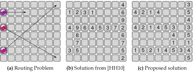
Example 3.1 Consider the situation depicted in Fig.3.1a. On a biochip of size 5×5, three droplets are to be routed. Droplet 3 should be moved from starting position (4,0)to an detecting device at position(3,4)while the other two droplets are to be routed to their common target at position(1,3). One possible solution of this routing problem using six time steps is shown in Fig.3.1b.
3.2
Complexity of Routing
This section will analyze the computational complexity of the DMFB Routing Problem. TheNP-completeness of the problem has already been conjectured in the literature. In [Böh04] the similarity to the NP-hard problem of moving multiple
© Springer International Publishing AG, part of Springer Nature 2019 O. Keszocze et al.,Exact Design of Digital Microfluidic Biochips,
https://doi.org/10.1007/978-3-319-90936-3_3
1
2
3
(a)
1
2
3
(b)
Fig. 3.1 Example for a routing problem with one possible solution. (a) Routing problem for three droplets: the biochip has a blockage of size 2×2 and a detecting device at position(3,4). (b) Exemplary routing solution using six time steps
robots has been noted ([CP08] uses a similar reasoning) while in [SHC06] the similarity to the Steiner Minimum Tree problem is pointed out. In this chapter, the (n2−1)-Puzzle will be used in an explicit proof of theNP-completeness of the DMFB Routing Problem.
Before being able to formally analyze the complexity of the routing problem, as defined in Definition3.1, it has to be formulated as a decision problem. The biochip will be modeled by a graph structure. The droplet routes then correspond to paths in that graph.
Definition 3.2 (DMFB Routing Problem as a Decision Problem) To formulate the routing problem as a decision problem, the formal graph model introduced in Sect.2.2is used. The interference region is modeled by another setI of edges.
Letp∗d, p†d ∈ V be the source and target position of the dropletd ∈ D. The net
containing dropletdis denotednd.
The decision problem is then defined as follows. Given a maximal number of time steps T ≥ 1, do there exist paths rd inG for alld, d′ ∈ D such that the
assertions
(rd(1)=pd∗)∧(rd(T )=pd†) (3.1)
and
{rd(t ), rd′(t−i)} ∈I (3.2)
fori=0,1 for dropletsd, d′withnd =nd′ and 1< t≤T hold?
3.2 Complexity of Routing 25
structure. That droplets which are not allowed to interfere with each other (that is, they belong to different nets) do not violate the fluidic constraints, is ensured via (3.2). The setI models the interference region. In the case ofrd(t )=rd′(t−0),
the constraint enforces that no two droplets are on the same cell at the same time step.
The decision problem definition of the DMFB Routing Problem is illustrated in the following example.
Example 3.2 Consider again the example shown in Fig.3.1. The problem descrip-tion and the soludescrip-tion using the formuladescrip-tion of Definidescrip-tion3.2is as follows.
The graphG=(V , E)is defined by the sets
V = {(x, y)|x, y∈ {0,1, . . . ,4}} \ {(1,1), (1,2), (2,1), (2,2)}
and
E= {{(x1, y1), (x2, y2)} |(x1, y1), (x2, y2)∈V ∧ |x1−x2| + |y1−y2| ≤1}.
The interference regions around the positions is modeled by
I = {{(x1, y1), (x2, y2)} |(x1, y1), (x2, y2)∈V ∧ |x1−x2| ≤1∧ |y1−y2| ≤1}.
The setI is the setEwith all the diagonally adjacent positions to be taken into consideration.
These sets, together with
p∗1=(0,4), p∗2=(2,0), p∗3=(4,1),
p1†=(1,3), p2†=(1,3), andp†3=(3,4),
describe the situation depicted in Fig.3.1a. The blockage of size 2×2 is modeled by removing the corresponding vertices from the graph.
The paths for the solution shown in Fig.3.1b are given by
r1=
(0,4), (1,4), (1,3), (1,3), (1,3), (1,3), (1,3)
,
r2=
(2,0), (1,0), (0,0), (0,1), (0,2), (0,3), (1,3)
, and
r3=
(4,1), (4,2), (4,3), (4,4), (3,4), (3,4), (3,4).
Theorem 3.1 The DMFB Routing Problem isNP-complete.
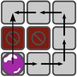
The proof of the Theorem is done via reduction of another, known-to-beNP -complete problem. The problem used is the(n2−1)-Puzzle defined below. Definition 3.3 ((n2−1)-Puzzle, [RW90]) The aim of the(n2−1)-Puzzle is to find a sequence of moves which will transfer a given initial configuration of ann×n board to a final (standard) configuration. A move consists of sliding a tile onto the empty square from an orthogonally adjacent square.
The question is: is there a solution for transforming the first (initial) configuration into the second (final) configuration requiring at mostkmoves?
Example 3.3 Consider the initial puzzle configuration in Fig.3.2a. The goal is to reach the configuration in Fig.3.2b in at mostksteps. It turns out that the smallest of suchkis 10.
As has been shown in [RW90], the (n2−1)-Puzzle is one of the many NP -complete problems. Its structure already closely resembles the routing problem on digital microfluidic biochips. With the definition of the puzzle, theNP-completeness of the DMFB Routing Problem can now be easily proven.
Proof (Proof of theNP-Completeness of the DMFB Routing Problem) As com-monly done in proofs forNP-completeness, see, for example, [GJ79], the proof is split into two parts. The first part proves that the problem lies withinNPby showing that it is possible to guess a solution for the problem and verify that solution (or prove that it is, in fact, no solution) in polynomial time. The second part reduces a knownNP-complete problem to the DMFB Routing Problem to show that it is at least as difficult as the reduced problem. Combining these parts concludes the proof that the DMFB Routing Problem isNP-complete.
The Droplet Routing Problem is inNP It is easy to guess a possible solution to the droplet routing problem. Algorithm1clearly verifies (or disproves) the solution in polynomial time. Assuming that the equality check can be performed in constant
1 8 2
4 3
7 6 5
(a)Start configuration of the 8-puzzle
1 2 3
4 5 6
7 8
(b)End configuration of the 8-puzzle
(c)8-Puzzle reduced to the DMFB Routing Problem
3.2 Complexity of Routing 27
Algorithm 1:Verify guessed DMFB routing solution Data: A DMFB Routing Problem (D,N, T , G=(V , E), I) Data: A possible solutionSof the droplet routing problem Result: Decision whetherSactually solves the problem 1 ford∈Ddo
2 if rd(1)=pd∗∨rd(T )=pd†then
// Incorrect start and end points
3 returnfalse;
4 for1< t≤T do
5 if{rd(t ), rd(t−1)} ∈Ethen
// Invalid droplet movement
6 returnfalse; 7 ford′∈D\nddo
8 if{rd(t ), rd′(t )} ∈I∨ {rd(t ), rd′(t−1)} ∈Ithen
// Fluidic constraint violation
9 returnfalse;
10 returntrue
time and that membership testing is linear in the size of the set, no more than #D· (2+T ·(#E+2·#I ·#D))steps have to be performed.
Reduction of(n2−1)to the Droplet Routing Problem The reduction is straightfor-ward. The board directly defines a quadratic biochip (see Example3.2for a similar biochip architecture) with
V = {0,1, . . . , n−1} × {0,1, . . . , n−1}
and
E= {{(x1, y1), (x2, y2)} |(x1, y1), (x2, y2)∈V ∧ |x1−x2| + |y1−y2| ≤1}.
The setI is chosen to contain the self-loops only. This means that the instance of the droplet routing only prevents multiple droplets on a single cell; no interference region around droplets is used. The dynamic fluidic constraints are still enforced, ensuring that only a single droplet moves in each time step. The tiles directly define the set of droplets; there is no multi-droplet net. That means thatD and N are given by
D= {1,2, . . . , n2−1} and N = {((d, p∗d), pd†)|d∈D}.
The solution to the droplet routing problem gives n2−1 routes that directly correspond to the solution of the(n2−1)-Problem.
One should note that the decision problem formulation does not directly solve the initial routing problem as it works on a fixed number of time steps. To actually use it to determine shortest routes, one needs to solve it repeatedly with an increasing T. This approach will be presented in detail in Sect.3.4.
3.3
Heuristic Approaches
As has been shown in the previous section, the routing problem is inherently difficult. This is reflected in the fact that mainly heuristic approaches for solving the routing problem have been proposed so far.
An early work on routing on DMFBs uses theA∗algorithm to route droplets on DMFBs [Böh04]. In order to cope with the state space explosion, the droplets are assigned priorities. The droplets are then routed sequentially in order of descending priority. This means that higher prioritized droplets are routed first. For the routing problem, already routed droplets of higher priority are treated as mobile blockages while droplets of lower priority are ignored since they have not been routed and, therefore, do not introduce any blockages. This work employs the static fluidic constraints but may produce very long routes for the droplet routed at last. The paper does not use the concept of nets meaning that only independent droplets are routed. The work [SHC06] does not only contribute the study of the fluidic constraints but also proposes a two-stage DMFB routing algorithm. The first step consists of determiningM alternative routes for each net. All of these routes adhere to a timing constraint. In the second step, routes for each net are randomly chosen. This scheme prevents issues with droplet priorities which could lead to poor routes for the least prioritized droplets. This problem is called the net-routing-order dependence problem. The chosen routes are then evaluated by using the number of cells used in the overall routing as a cost function. Furthermore, the solution is checked for fluidic constraint violations. This process is repeated an adequate number of times until the set of routes with the minimum cost value is chosen.
In [CP08], the authors introduce the concepts of bypassibility for droplets and concession zones to which droplets can be routed in order to break up a deadlock. The main idea is to route the droplets in the order chosen by the bypassibility value. The non-routed droplets are then seen as blockages making the search space for the algorithm two-dimensional as no timing information is necessary. This work uses a slightly less restrictive version of the fluidic constraints, effectively putting only the horizontal and vertical neighbors of a cell in the interference region. This means that the interference region and the reachable positions are identical (meaning that in both cases the region as shown in Fig.2.2a from Sect.2.1.2is used). In terms of the graph representation of the routing problem, this means thatIandEare identical.
3.4 Proposed Solution 29
routing step, the approach is to iteratively search for a set of independent nets which then are routed using a network-flow-based algorithm order of decreasing criticality. This routing is performed on a “coarser” biochip which consists of cells representing a 3×3 array of cells on the original biochip. After all nets have been globally routed, the detailed routing part employs a negotiation-based algorithm that routes the droplets in decreasing order of criticality. This approach is not capable of directly handling 3-nets. It splits them into two 2-nets prior to routing.
The work [HH09] features an entropy-based algorithm for routing that makes use of preferred routing paths. The authors explicitly tackle the problem of droplet routing order by sorting the droplets based on the congestion of the routing regions. To model this, they borrow the notion of entropy from the field of thermodynamics, routing droplets with a higher variant in the entropy first. The main idea of this work is to mark rows and columns as preferred routing directions, penalizing droplets not directly following them. In a post-processing step, the routes are transformed into a one-dimensional representation and compacted using a dynamic programming approach. This work uses the same less restrictive version of the fluidic constraints as [CP08].
While all these heuristic approaches solve the routing problem, they cannot guarantee the minimality of the routes. This allows for relative comparisons between these approaches only. So far, it is not known how close to the technical optimum the solutions generated by these methods are. When transporting liquids that degrade over time, the minimality of routes can be of utmost importance.
Another aspect that is not addressed by these approaches is the correctness of the solutions. In classical circuit design, vendors validate their solutions using another tool from a different tool vendor to ensure that their netlists are indeed correct. While the presented methodologies most likely produce correct solutions, there is no guarantee.
3.4
Proposed Solution
The methodology proposed in this section (originally introduced in [KWD14]), in contrast to prior work, is non-heuristic and exact. The decision problem formulation from Sect.3.2is the main part of the proposed methodology. As already mentioned, a single decision problem is not sufficient for solving the routing problem. The general idea is to formalize the routing problem as a series of decision problems asking “Does there exist a routing inT time steps?” with an increasingT. This leads to the following, simple solving scheme:
1. SetT =1.
Of course, if there is some a-priori knowledge about the minimal route length, the initialization ofT can be adjusted accordingly.
The proposed approach has the following properties.
Correctness The generated solutions are correct-by-construction with respect to the underlying model. This means that there is no need to further verify the solutions.
Minimality As the iteration scheme starts with the minimal number of time steps and then iteratively increases it, finding the solution using the minimal number of time steps is guaranteed.
This guarantee is not just an important characteristic for concrete routing solutions but also allows to createground truthfor a variety of comparisons like the evaluation of heuristic approaches.
Abstraction A formal model of the domain helps to understand the considered problems. The proposed approach is directly derived from the abstract model introduced in Sect.2.2. This effectively frees the researcher from finding algo-rithms herself.
The proposed methodology inherently avoids problems like the net-routing order dependence problem (see Sect.3.3) without resorting to workarounds such as splitting nets to work on 2-nets only.
Solving Time As has been shown, the problem isNP-complete. This means that finding an optimal solution to the DMFB Routing Problem will take time. Instead of spending a lot of time, trying to find a good algorithm for solving the routing problem, a highly optimized solving engine is employed instead.
As the underlying technology to solve the decision problem, SAT (see Sect.2.3) has been chosen. This means that the formal model is translated into a SAT instance that is then solved using an appropriate solver.
Creating a SAT instance is a two-step process. At first, the SAT variables used must be defined. In the second step, these variables are constrained to express states that adhere to the model only.
3.4.1
SAT Variables
To fully model the DMFB Routing Problem, Boolean variables that represent whether a certain droplet is present on a given cell position at a given time step are sufficient. That is, Boolean variables denoted
cp,d (3.3)
3.4 Proposed Solution 31
Fig. 3.3 Visualization of the third time step with exemplary variable assignment for the routing solution depicted in Fig.3.1b. (a) Third time step of the routing solution. (b) Boolean variables and their assignments (excerpt)
How these variables are used to describe a configuration of a routing is illustrated in the following example.
Example 3.5 Consider again the routing problem and its solution from Fig.3.1. The set of all cell positions is given byP = {0,1,2,3,4} × {0,1,2,3,4}, the set of droplets is given byD= {1,2,3}and the set of nets is given by
N = {({(1, (0,4)), (2, (2,0))}, (1,3)), ({(3, (4,1))}, (3,4))}.
Figure3.3a displays the third time step of the routing solution (the third time step means that the droplets have moved twice). The droplets’ positions are given by p1=(1,3), p2=(0,0), andp3=(4,3). Figure3.3b shows a representative subset of SAT variables as defined in (3.3) and their assignments. The blockage is realized by assigning all variables that correspond to the blocked positions the valuefalse.
3.4.2
SAT Constraints
In the following, constraints covering various aspects of routing are introduced and explained. The total of all these constraints then define the decision problem used in the iterative solving scheme.
Source and Target Configuration
In the first time step, the droplets are explicitly positioned on their target positions by directly setting the values of the corresponding SAT variables totrueusing the constraints
d∈D c1p∗
d,d. (3.4)
To ensure that the droplets reach their target positions, the constraints
are added to the SAT instance. Note that there is no specific time step in which the droplets are expected to be at their position. Only the fact that they eventually will is encoded. That means that droplets needing few time steps to reach their target may have left their target in the last time step.
Droplet Movement
A droplet may not arbitrarily appear on a cell on the biochip. It can only be present at a cell positionpif it was already present in the neighborhoodN (p)of horizontally and vertically adjacent positions of that particular positionpin the previous time step (see Fig.2.2a for a visualization). This situation is depicted in Fig.3.4. The corresponding constraints are
The constraints model the movement of droplets starting with the second time step. This is necessary as the variablectp−′,d1 would be undefined fort =1. The positions
at the first time step are already fixed by (3.4).
3.4 Proposed Solution 33
To avoid unintentional mixing, dropletsd andd′ that do not share a common net nmust not enter each other’s interference region. This means that d′ must avoid the interference regionNI(d)(see Fig.2.2b for a visualization). This applies to the
current time step as well as the previous one. This is formulated as follows:
removed from the constraint. For the sake of simplicity and readability, (3.7) does not explicitly depict this.
The common net sizes are 2-nets and 3-nets. Nevertheless, the presented routing method is technically capable of handling nets of arbitrary size.
Blockages and Consistency
To make the droplets respect the blockages on the biochip, the simple constraints
are sufficient. The SAT variables for all droplets and time steps that correspond to blockages are directly set tofalse.
To ensure that a droplet is present at most once, the constraints
that do not fixate a droplet on its target once it has been reached. The movement constraints from (3.6) make sure that a droplet does not re-appear on the biochip.
3.5
Experimental Results
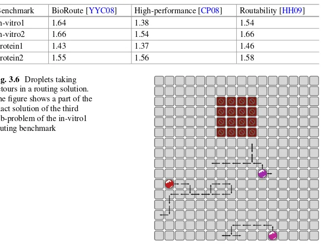
To evaluate the proposed methodology, its results are compared against the results of the approaches presented in Sect.3.3. Experimental results have been gener-ated for benchmarks commonly used in evaluating DMFB routing algorithms. The benchmark sets are described in [SC05] and [SHC06]. The benchmarks are organized in four sets containing multiple sub-problems. The in-vitro benchmarks describe a typical multiplexed experiment. The three human fluids samples urine, serum, and plasma are mixed with the reagents glucose oxidase and lactase oxidase and, afterwards, analyzed. This experiment is based on Trinder’s reaction, for details see [Tri69]. In the protein experiments, samples with proteins are diluted. Afterwards, they are mixed with reagents for reaction. In the last step, the protein concentration is analyzed. For details on the experiment, see [Sri+04]. Figure3.5 shows the second sub-problem of the in-vitro1 benchmark set. Table3.1summarizes the characteristics of the benchmarks.
The constraints of the previous section have been implemented in C++ using Z3 [DB08] as the SAT solver. The cardinality constraints of (3.9) were implemented using the scheme of [Sin05]. The experiments were run on a machine with four Intel Xeon CPUs at 3.50 GHz and 32 Gb RAM running Fedora 22.
Unfortunately, the proposed methodology cannot directly be compared against all approaches reviewed in Sect.3.3. The work [SHC06] shows the applicability of the approach on a use case only. Furthermore, the results of [YYC08] that display the maximal route length as well as the average route length had to be taken from [HH09]. As the related work uses 0 as the first time step, their results have been adjusted to be comparable to the presented approach.
(a) (b)
3.5 Experimental Results 35
Table 3.1 Characteristics of the benchmarks
Benchmark Biochip size # sub-problems # nets maxd
in-vitro1 16×16 11 28 5
in-vitro2 14×14 15 35 6
protein1 21×21 64 181 6
protein2 13×13 78 178 6
#sub-problems: the number of sub-problems in the benchmark set, # nets: total number of nets in benchmark set, maxd: maximal number of droplets in a sub-problem
Table 3.2 Comparison of proposed method with methods that use the fluidic constraints as defined in [SHC06]
BioRoute [YYC08] Proposed
Benchmark T ∅T #c T ∅T #c Dur (s)
in-vitro1 21 14.00 237 20 13.00 387 98.44
in-vitro2 18 12.33 236 17 11.07 391 62.39
protein1 21 17.31 1618 21 16.28 2318 1074.50
protein2 21 11.51 939 21 10.54 1455 172.24
T: maximal number of time steps needed,∅T: average number of time steps needed, #c: number of used cells, Dur (s): time needed to solve the routing problems in seconds
Table 3.3 Comparison of proposed method with methods that use less restrictive fluidic con-straints
High-performance Routability
[CP08] [HH09] Proposed
Benchmark T ∅T #c T ∅T #c T ∅T #c dur (s)
in-vitro1 20 15.30 258 19 13.47 231 19 12.82 356 65.43
in-vitro2 21 13.00 246 18 11.43 229 17 11.07 379 49.13
protein1 21 17.55 1688 21 16.51 1588 21 16.28 2315 902.23
protein2 21 13.19 936 21 11.04 923 21 10.53 1456 132.67
T: maximal number of time steps needed,∅T: average number of time steps needed, #c: number
of used cells, Dur (s): time needed to solve the routing problems in seconds
No related work provides results for the individual sub-problems. Therefore, following the methodology of the other publications, the results are presented in aggregated manner. This means that for all four benchmark sets the maximal number of time steps needed to solve all sub-problems, the average number of time steps as well as the total number of used cells is reported.
As different authors use different versions of the fluidic constraints (see Sect.3.3), (3.7) has been adapted accordingly. The difference is whether the diagonally adjacent positions are considered in the interference region. To incorporate this difference, the use of the neighborhoodNI(p)in (3.7) is changed
![Fig. 1.2 Physical realizationof a flow-based biochip of thesize of a dime [Whi06,Figure 1]](https://thumb-ap.123doks.com/thumbv2/123dok/3939754.1883174/12.439.169.386.60.401/fig-physical-realizationof-ow-based-biochip-thesize-figure.webp)
![Figure 13])34](https://thumb-ap.123doks.com/thumbv2/123dok/3939754.1883174/65.439.169.387.59.407/figure.webp)