FOURIER SERIES AND INTEGRALS
4.1
FOURIER SERIES FOR PERIODIC FUNCTIONS
This section explains three Fourier series: sines, cosines, and exponentials eikx. Square waves (1 or 0 or−1) are great examples, with delta functions in the derivative. We look at a spike, a step function, and a ramp—and smoother functions too.
Start with sinx. It has period 2π since sin(x+ 2π) = sinx. It is an odd function since sin(−x) = −sinx, and it vanishes atx= 0 andx =π. Every function sinnx
has those three properties, and Fourier looked atinfinite combinations of the sines:
Fourier sine series S(x) =b1sinx+b2sin 2x+b3sin 3x+· · ·= ∞
n=1
bnsinnx (1)
If the numbers b1, b2, . . . drop off quickly enough (we are foreshadowing the im-portance of the decay rate) then the sumS(x) will inherit all three properties:
Periodic S(x+ 2π) =S(x) Odd S(−x) =−S(x) S(0) =S(π) = 0
200 years ago, Fourier startled the mathematicians in France by suggesting thatany function S(x) with those properties could be expressed as an infinite series of sines. This idea started an enormous development of Fourier series. Our first step is to compute fromS(x) the numberbkthat multiplies sinkx.
Suppose S(x) =
bnsinnx. Multiply both sides by sinkx. Integrate from 0to π:
π
0
S(x) sinkx dx= π
0
b1sinxsinkx dx+· · ·+ π
0
bksinkx sinkx dx+· · · (2)
On the right side, all integrals are zero except the highlighted one with n = k. This property of “orthogonality” will dominate the whole chapter. The sines make 90◦
angles in function space, when their inner products are integrals from 0 toπ:
Orthogonality
π
0
sinnx sinkx dx= 0 if n=k . (3)
Zero comes quickly if we integrate
The highlighted term in equation (2) isbkπ/2. Multiply both sides of (2) by 2/π:
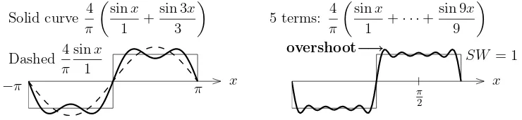
Sine coefficients I will go immediately to the most important example of a Fourier sine series. S(x) is anodd square wavewithSW(x) = 1 for 0< x < π. It is drawn in Figure 4.1 as
Example 1 Find the Fourier sine coefficients bk of the square waveSW(x).
Solution Fork= 1,2, . . .use the first formula(6)withS(x) = 1between0andπ:
The even-numbered coefficients b2k are all zero because cos 2kπ = cos 0 = 1. The
odd-numbered coefficientsbk= 4/πkdecrease at the rate 1/k. We will see that same 1/k decay rate for all functions formed fromsmooth pieces and jumps.
Put those coefficients 4/πk and zero into the Fourier sine series forSW(x):
Square wave SW(x)= 4
include more terms. Away from the jumps, we safely approach SW(x) = 1 or −1. Atx=π/2, the series gives a beautiful alternating formula for the numberπ:
1 = 4
The Gibbs phenomenon is the overshoot that moves closer and closer to the jumps. Its height approaches 1.18. . . and it does not decrease with more terms of the series! Overshoot is the one greatest obstacle to calculation of all discontinuous functions (like shock waves in fluid flow). We try hard to avoid Gibbs but sometimes we can’t.
x x
Figure 4.2: Gibbs phenomenon: Partial sums N
1 bnsinnxovershoot near jumps.
Fourier Coefficients are Best
Let me look again at the first termb1sinx= (4/π) sinx. This is theclosest possible approximationto the square waveSW, by any multiple of sinx(closest in the least squares sense). To see this optimal property of the Fourier coefficients, minimize the error over allb1: This is exactly equation (6) for the Fourier coefficient.
Eachbksinkxis as close as possible toSW⊛. We can find the coefficientsbk one
at a time,because the sines are orthogonal. The square wave hasb2 = 0 because all other multiples of sin 2x increase the error. Term by term, we are “projecting the function onto each axis sinkx.”
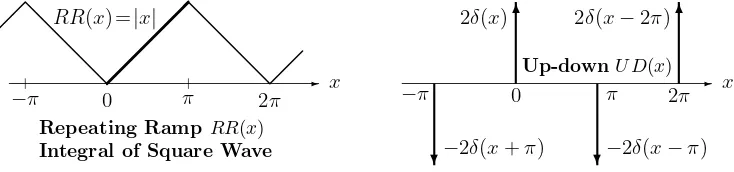
Every cosine has period 2π. Figure 4.3 shows two even functions, therepeating ramp RR(x) and the up-down train UD(x) of delta functions. That sawtooth ramp RR is the integral of the square wave. The delta functions in UD give the derivative of the square wave. (For sines, the integral and derivative are cosines.)
RRandUD will be valuable examples, one smoother thanSW, one less smooth. First we find formulas for the cosine coefficientsa0andak. The constant terma0 is theaverage value of the functionC(x):
a0 =Average a0= 1
π
π
0
C(x)dx= 1 2π
π
−πC(x)dx. (11)
I just integrated every term in the cosine series (10) from 0 toπ. On the right side, the integral ofa0is a0π (divide both sides byπ). All other integrals are zero:
π
0
cosnx dx=
sinnx n
π
0
= 0−0 = 0. (12)
In words, the constant function 1 is orthogonal to cosnxover the interval [0, π]. The other cosine coefficientsak come from the orthogonality of cosines. As with sines, we multiply both sides of (10) by coskxand integrate from 0 toπ:
π
0
C(x) coskx dx= π
0
a0coskx dx+ π
0
a1cosxcoskx dx+··+ π
0
ak(coskx)2 dx+··
You know what is coming. On the right side, only the highlighted term can be nonzero. Problem 4.1.1 proves this by an identity for cosnxcoskx—now (4) has a plus sign. The bold nonzero term isakπ/2and we multiply both sides by 2/π:
Cosine coefficients
C(−x) =C(x) ak= 2
π
π
0
C(x) coskx dx= 1
π
π
−π
C(x) coskx dx . (13)
Again the integral over a full period from−π toπ (also 0 to 2π) is just doubled.
✲ x
−π 0 π 2π
RR(x) =|x|
Repeating RampRR(x)
Integral of Square Wave
✲
❄
✻
❄
✻
x
−π 0 π 2π
−2δ(x+π) 2δ(x)
−2δ(x−π) 2δ(x−2π)
Up-downU D(x)
Example 2 Find the cosine coefficients of the ramp RR(x)and the up-down UD(x).
Solution The simplest way is to start with the sine series for the square wave:
SW(x) = 4
π
sinx
1 + sin 3x
3 +
sin 5x
5 +
sin 7x
7 +· · · .
Take the derivative of every term to produce cosines in the up-down delta function:
Up-down series UD(x) = 4
π[cosx+ cos 3x+ cos 5x+ cos 7x+· · ·]. (14)
Those coefficients don’t decay at all. The terms in the series don’t approach zero, so officially the series cannot converge. Nevertheless it is somehow correct and important. Unofficially this sum of cosines has all1’s at x= 0 and all−1’s at x =π. Then+∞ and−∞ are consistent with2δ(x) and −2δ(x−π). The true way to recognize δ(x) is by the test
δ(x)f(x)dx=f(0)and Example 3 will do this.
For the repeating ramp, we integrate the square wave series forSW(x) and add the average ramp heighta0=π/2, halfway from0to π:
Ramp series RR(x)= π 2−
π
4
cosx
12 + cos 3x
32 + cos 5x
52 + cos 7x
72 +· · · . (15) The constant of integration isa0. Those coefficientsakdrop off like 1/k2. They could be computed directly from formula(13)using
xcoskx dx, but this requires an integration by parts (or a table of integrals or an appeal toMathematica orMaple). It was much easier to integrate every sine separately inSW(x), which makes clear the crucial point:
Each “degree of smoothness” in the function is reflected in a faster decay rate of its Fourier coefficientsak and bk.
No decay Deltafunctions (with spikes) 1/k decay Stepfunctions (with jumps) 1/k2
decay Rampfunctions (with corners) 1/k4
decay Spline functions (jumps inf′′′ ) rk decay with r <1 Analyticfunctions like 1/(2
−cosx)
Each integration divides thekth coefficient byk. So the decay rate has an extra 1/k. The “Riemann-Lebesgue lemma” says that ak and bk approach zero for any continuous function (in fact whenever
|f(x)|dxis finite). Analytic functions achieve a new level of smoothness—they can be differentiated forever. Their Fourier series and Taylor series in Chapter 5 convergeexponentially fast.
The poles of 1/(2−cosx) will be complex solutions of cosx= 2. Its Fourier series converges quickly becauserk decays faster than any power 1/kp. Analytic functions
are ideal for computations—the Gibbs phenomenon will never appear.
Example 3 Find the (cosine) coefficients of thedelta function δ(x), made2π-periodic.
Solution The spike occurs at the start of the interval [0, π] so safer to integrate from −πto π. We find a0= 1/2πand the other ak= 1/π(cosines because δ(x)is even):
Average a0= 1 2π
π
−π
δ(x)dx= 1
2π Cosines ak= 1
π
π
−π
δ(x) coskx dx= 1 π
Then the series for the delta function has all cosines in equal amounts:
Delta function δ(x) = 1 2π+
1
π[cosx+ cos 2x+ cos 3x+· · ·]. (16)
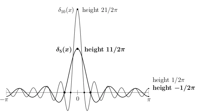
Again this series cannot truly converge (its terms don’t approach zero). But we can graph the sum aftercos 5xand after cos 10x. Figure 4.4 shows how these “partial sums” are doing their best to approachδ(x). They oscillate faster and faster away fromx= 0.
Actually there is a neat formula for the partial sumδN(x)that stops atcosNx. Start
by writing each term2 cosθ as eiθ+e−iθ :
δN = 1
2π[1 + 2 cosx+· · ·+ 2 cosNx] =
1 2π
1 +eix+e−ix
+· · ·+eiN x+e−iN x
.
This is a geometric progression that starts frome−iN x
and ends ateiN x. We have powers
of the same factoreix. The sum of a geometric series is known:
Partial sum
up to cosN x δN(x) = 1 2π
ei(N+1
2)x−e−i(N+12)x
eix/2−e−ix/2 = 1 2π
sin(N+12)x
sin12x . (17)
This is the function graphed in Figure 4.4. We claim that for anyN the area underneath
δN(x) is 1. (Each cosine integrated from −π to π gives zero. The integral of 1/2π is
1.) The central “lobe” in the graph ends when sin(N + 1
2)x comes down to zero, and that happens when(N+12)x=±π. I think the area under that lobe (marked by bullets) approaches the same number1.18. . .that appears in the Gibbs phenomenon.
In what way doesδN(x)approachδ(x)? The termscosnx in the series jump around
at each pointx= 0, not approaching zero. Atx=πwe see 21π[1−2 + 2−2 +· · ·]and the sum is1/2π or−1/2π. The bumps in the partial sums don’t get smaller than1/2π. The right test for the delta functionδ(x)is to multiply by a smoothf(x) =
akcoskx
and integrate, becausewe only know δ(x)from its integrals
δ(x)f(x)dx=f(0):
Weak convergence of δN(x) to δ(x)
π
−π
δN(x)f(x)dx=a0+· · ·+aN →f(0). (18)
In this integrated sense (weak sense) the sumsδN(x)do approach the delta function !
The convergence ofa0+· · ·+aN is the statement that at x= 0 the Fourier series of a
smoothf(x) =
−π 0 π
δ5(x)
δ10(x)
height 11/2π height 21/2π
height−1/2π height 1/2π
Figure 4.4: The sumsδN(x) = (1 + 2 cosx+· · ·+ 2 cosNx)/2πtry to approachδ(x).
Complete Series: Sines and Cosines
Over the half-period [0, π], the sines are not orthogonal to all the cosines. In fact the integral of sinx times 1 is not zero. So for functionsF(x) that are not odd or even, we move to the complete series (sines plus cosines) on the full interval. Since our functions are periodic, that “full interval” can be [−π, π] or [0,2π]:
Complete Fourier series F(x) =a0+ ∞
n=1
ancosnx+ ∞
n=1
bnsinnx . (19)
On every “2πinterval” all sines and cosines are mutually orthogonal. We find the Fourier coefficientsak andbk in the usual way: Multiply(19)by1and coskxand sinkx, and integrate both sides from−π toπ:
a0 = 1 2π
π
−π
F(x)dx ak= 1
π
π
−π
F(x) coskx dx bk= 1
π
π
−π
F(x) sinx dx. (20)
Orthogonality kills off infinitely many integrals and leaves only the one we want. Another approach is to split F(x) =C(x) +S(x) into an even part and an odd part. Then we can use the earlier cosine and sine formulas. The two parts are
C(x) =Feven(x) =
F(x) +F(−x)
2 S(x) =Fodd(x) =
F(x)−F(−x)
2 . (21)
Example 4 Find thea’s andb’s ifF(x) =square pulse=
Coefficients of square pulse a0= 1
When h approaches zero, F(x)/h is squeezed into a very thin interval. The tall rectangle approaches (weakly) the delta functionδ(x). The average height is area/2π= 1/2π. Its other coefficients ak/handbk/happroach1/πand0, already known for δ(x):
When the function has a jump, its Fourier series picks the halfway point. This example would converge toF(0) = 1
2 andF(h) = 1
2, halfway up and halfway down. The Fourier series converges toF(x) at each point where the function is smooth. This is a highly developed theory, and Carleson won the 2006 Abel Prize by proving convergence for everyxexcept a set of measure zero. If the function has finite energy
|F(x)|2dx, he showed that the Fourier series converges “almost everywhere.”
Energy in Function
=
Energy in Coefficients
There is an extremely important equation (the energy identity) that comes from integrating (F(x))2. When we square the Fourier series ofF(x), and integrate from −π to π, all the “cross terms” drop out. The only nonzero integrals come from 12 and cos2kx and sin2kx, multiplied bya2
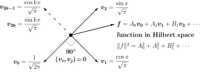
The energy in F(x) equals the energy in the coefficients. The left side is like the length squared of a vector, exceptthe vector is a function. The right side comes from an infinitely long vector of a’s and b’s. The lengths are equal, which says that the Fourier transform from function to vector is like an orthogonal matrix. Normalized by constants√2π and√π, we have an orthonormal basis in function space.
What is this function space ? It is like ordinary 3-dimensional space, except the “vectors” are functions. Their lengthfcomes from integrating instead of adding: f2=
Lengthf2= (f, f) comes from the inner product (f, g) =
f(x)g(x)dx
Orthogonal functions (f, g) = 0 produce a right triangle: f+g2=f2+g2
I have tried to draw Hilbert space in Figure 4.5. It has infinitely many axes. The energy identity (24)is exactly the Pythagoras Law in infinite-dimensional space.
✒
Figure 4.5: The Fourier series is a combination of orthonormalv’s (sines and cosines).
Complex Exponentials
c
ke
ikxThis is a small step and we have to take it. In place of separate formulas fora0andak andbk, we will haveone formulafor all the complex coefficientsck. And the function
F(x) might be complex (as in quantum mechanics). The Discrete Fourier Transform will be much simpler when we useN complex exponentials for a vector. We practice in advance with the complex infinite series for a 2π-periodic function:
Complex Fourier series F(x) =c0+c1eix+c−1e Then (25) is the sine series for an odd function and thec’s are pure imaginary.
To findck, multiply (25) bye−ikx
(noteikx)and integrate from
−π toπ:
Notice thatc0 =a0 is still the average of F(x), because e0 = 1. The orthogonality ofeinx and eikx is checked by integrating, as always. But the complex inner product
(F, G) takes thecomplex conjugate G ofG. Before integrating, changeeikx toe−ikx :
Complex inner product Orthogonality of einx and eikx
(F, G) = series have exponentially fast decay from1/2k. The functions are analytic.
When we add those functions, we get a real analytic function:
1
This ratio is the infinitely smooth function whose cosine coefficients are1/2k.
Example 6 Findckfor the2π-periodic shifted pulseF(x) =
Notice above all the simple effect of the shift by s. It “modulates” eachckby e−iks . The energy is unchanged, the integral of|F|2just shifts, and all|e−iks
|= 1:
Shift F(x) to F(x−s) ←→ Multiply ck by e−iks. (30)
Example 7 Centered pulsewith shifts=−h/2. The square pulse becomes centered aroundx= 0. This even function equals1on the interval from−h/2to h/2:
That division byh produces area = 1. Every coefficient approaches 1
Hilbert space can contain vectors c= (c0, c1, c−1, c2, c−2,· · ·) instead of functions
F(x). The length of cis 2π |ck|2=
|F|2dx. The function space is often denoted byL2and the vector space isℓ2. The energy identity is trivial (but deep). Integrating the Fourier series forF(x) timesF(x), orthogonality kills every cnckforn=k. This leaves theckck=|ck|2:
π
−π
|F(x)|2dx= π
−π
(cneinx)(cke−ikx
)dx= 2π(|c0|2+|c1|2+|c−1|2+··). (31)
This is Plancherel’s identity: The energy inx-space equals the energy in k-space.
Finally I want to emphasize the three big rules for operating onF(x) =
ckeikx:
1. The derivative dF
dx has Fourier coefficientsikck(energy moves to highk).
2. The integral of F(x)has Fourier coefficients ck
ik, k= 0 (faster decay).
3. The shift toF(x−s)has Fourier coefficientse−iks
ck(no change in energy).
Application: Laplace’s Equation in a Circle
Our first application is to Laplace’s equation. The idea is to constructu(x, y) as an infinite series, choosing its coefficients to matchu0(x, y) along the boundary. Every-thing depends on the shape of the boundary, and we take a circle of radius 1.
Begin with the simple solutions 1,rcosθ,rsinθ,r2cos 2θ,r2sin 2θ, ... to Laplace’s equation. Combinations of these special solutions give all solutions in the circle:
u(r, θ) =a0+a1rcosθ+b1rsinθ+a2r2cos 2θ+b2r2sin 2θ+· · · (32)
It remains to choose the constants ak and bk to make u = u0 on the boundary. For a circleu0(θ) is periodic, sinceθ andθ+ 2π give the same point:
Setr= 1 u0(θ) =a0+a1cosθ+b1sinθ+a2cos 2θ+b2sin 2θ+· · · (33)
This is exactly the Fourier series foru0. The constantsak and bk must be the Fourier coefficients of u0(θ). Thus the problem is completely solved, if an infinite series (32) is acceptable as the solution.
Example 8 Point sourceu0=δ(θ)at θ= 0 The whole boundary is held atu0= 0, except for the source atx= 1,y= 0. Find the temperatureu(r, θ)inside.
Fourier series forδ u0(θ) = 1 2π+
1
π(cosθ+ cos 2θ+ cos 3θ+· · ·) =
1 2π
∞
−∞
Inside the circle, eachcosnθ is multiplied byrn:
Infinite series foru u(r, θ) = 1 2π +
1
π(rcosθ+r
2cos 2θ+r3cos 3θ+
· · ·) (34)
Poisson managed to sum this infinite series! It involves a series of powers of reiθ.
So we know the response at every(r, θ)to the point source atr= 1, θ= 0:
Temperature inside circle u(r, θ) = 1 2π
1−r2
1 +r2−2rcosθ (35)
At the centerr= 0, this produces the average ofu0=δ(θ) which isa0= 1/2π. On the boundaryr= 1, this producesu= 0except at the point source where cos 0 = 1:
On the ray θ= 0 u(r, θ) = 1 2π
1−r2 1 +r2−2r =
1 2π
1 +r
1−r. (36)
Asrapproaches1, the solution becomes infinite as the point source requires.
Example 9 Solve for any boundary valuesu0(θ)by integrating over point sources. When the point source swings around to angle ϕ, the solution (35) changes from θ to
θ−ϕ. Integrate this “Green’s function” to solve in the circle:
Poisson’s formula u(r, θ) = 1 2π
π
−π
u0(ϕ) 1−r
2
1 +r2−2rcos(θ−ϕ) dϕ (37)
Ar r = 0 the fraction disappears and u is the average
u0(ϕ)dϕ/2π. The steady state temperature at the center is the average temperature around the circle.
Poisson’s formula illustrates a key idea. Think of anyu0(θ)as a circle of point sources. The source at angle ϕ = θ produces the solution inside the integral (37). Integrating around the circle adds up the responses to all sources and gives the response tou0(θ).
Example 10 u0(θ) = 1on the top half of the circle andu0=−1on the bottom half.
Solution The boundary values are the square wave SW(θ). Its sine series is in (8):
Square wave for u0(θ) SW(θ) = 4
π
sinθ
1 + sin 3θ
3 +
sin 5θ
5 +· · · (38)
Inside the circle, multiplying byr, r2,r3,... gives fast decay of high frequencies:
Rapid decay inside u(r, θ) = 4
π
rsinθ
1 +
r3sin 3θ
3 +
r5sin 5θ
5 +· · · (39)
WORKED EXAMPLE
A hot metal bar is moved into a freezer (zero temperature). The sides of the bar are coated so that heat only escapes at the ends. What is the temperature u(x, t) along the bar at timet? It will approach u= 0 as all the heat leaves the bar.
Solution The heat equation is ut = uxx. At t= 0 the whole bar is at a constant
temperature, sayu= 1. The ends of the bar are at zero temperature for all timet >0. This is aninitial-boundary value problem:
Heat equation ut=uxx with u(x,0) = 1 and u(0, t) =u(π, t) = 0. (40)
Those zero boundary conditions suggest a sine series. Its coefficients depend ont:
Series solution of the heat equation u(x, t) = ∞
1
bn(t) sinnx. (41)
The form of the solution showsseparation of variables. In a comment below, we look for productsA(x)B(t) that solve the heat equation and the boundary conditions. What we reach is exactlyA(x) = sinnxand the series solution (41).
Two steps remain. First, choose eachbn(t) sinnxto satisfy the heat equation:
Substitute intout=uxx b′
n(t) sinnx=−n2bn(t) sinnx bn(t) =e
−n2t
bn(0).
Noticeb′
n=−n2bn. Now determine eachbn(0) from the initial conditionu(x,0) = 1
on (0, π). Those numbers are the Fourier sine coefficients ofSW(x) in equation (38):
Box function/square wave
∞
1
bn(0) sinnx= 1 bn(0) = 4
πn for oddn
This completes the series solution of the initial-boundary value problem:
Bar temperature u(x, t) = oddn
4
πne
−n2t
sinnx. (42)
For large n (high frequencies) the decay of e−n2t
is very fast. The dominant term (4/π)e−t
sinx for large times will come from n = 1. This is typical of the heat equation and all diffusion, that the solution (the temperature profile) becomes very smooth astincreases.
Numerical difficulty I regret any bad news in such a beautiful solution. To compute
Those unphysical bumps are precisely the Gibbs phenomenon. The initial
u(x,0) is 1 on (0, π) but its odd reflection is−1 on (−π,0). That jump has produced the slow 4/πndecay of the coefficients, with Gibbs oscillations nearx= 0 andx=π. The sine series foru(x, t) is not a success numerically. Would finite differences help?
Separation of variables We foundbn(t) as the coefficient of an eigenfunction sinnx. Another good approach is to putu=A(x)B(t) directly intout=uxx:
Separation A(x)B′(t) =A′′(x)B(t) requires A′′(x)
A(x) =
B′(t)
B(t) =constant. (43)
A′′/Ais constant in space,B′/B is constant in time, and they are equal:
A′′
A =−λgivesA= sin
√
λ xand cos√λ x B′
B =−λ givesB=e
−λt
The productsAB =e−λt
sin√λ xand e−λt
cos√λ x solve the heat equation for any number λ. But the boundary condition u(0, t) = 0 eliminates the cosines. Then
u(π, t) = 0 requiresλ=n2= 1,4,9, . . .to have sin√λ π= 0. Separation of variables has recovered the functions in the series solution (42).
Finallyu(x,0) = 1 determines the numbers 4/πnfor oddn. We find zero for even
nbecause sinnxhasn/2 positive loops andn/2 negative loops. For oddn, the extra positive loop is a fraction 1/nof all loops, giving slow decay of the coefficients. Heat bath (the opposite problem) The solution on the website is 1−u(x, t), because it solves a different problem. The bar is initially frozen at U(x,0) = 0. It is placed into a heat bath at the fixed temperature U = 1 (or U = T0). The new unknown isU and its boundary conditions are no longer zero.
The heat equation and its boundary conditions are solved first by UB(x, t). In this exampleUB≡1 is constant. Then the differenceV =U−UB has zero boundary values, and its initial values areV = −1. Now the eigenfunction method (or sepa-ration of variables) solves forV. (The series in (42) is multiplied by −1 to account forV(x,0) =−1.) Adding back UB solves the heat bath problem: U =UB +V = 1−u(x, t).
HereUB ≡1 is thesteady statesolution att=∞, andV is thetransient solution. The transient starts atV =−1 and decays quickly toV = 0.
Heat bath at one end The website problem is different in another way too. The Dirichlet conditionu(π, t) = 1 is replaced by the Neumann condition u′(1, t) = 0. Only the left end is in the heat bath. Heat flows down the metal bar and out at the far end, now located atx= 1. How does the solution change for fixed-free?
AgainUB = 1 is a steady state. The boundary conditions apply toV = 1−UB:
Fixed-free
eigenfunctions V(0) = 0 and V′(1) = 0 lead to A(x) = sin
n+1 2
Those eigenfunctions give a new form for the sum ofBn(t)An(x):
Fixed-free solution V(x, t) = oddn
Bn(0)e−(n+1
2)2π2t sin
n+1 2
πx. (45)
All frequencies shift by 1
2 and multiply by π, because A′′ = −λA has a free end atx = 1. The crucial question is: Does orthogonality still hold forthese new eigenfunctions sin
n+12
πx on [0,1]? The answer is yes because this fixed-free “Sturm–Liouville problem”A′′=−λAis still symmetric.
Summary The series solutions all succeed but the truncated series all fail. We can see the overall behavior of u(x, t) and V(x, t). But their exact values close to the jumps are not computed well until we improve on Gibbs.
We could have solved the fixed-free problem on [0,1] with the fixed-fixed solution on [0,2]. That solution will be symmetric around x = 1 so its slope there is zero. Then rescalingx by 2π changes sin(n+1
2)πx into sin(2n+ 1)x. I hope you like the graphics created by Aslan Kasimov on thecsewebsite.
Problem Set 4.1
1 Find the Fourier series on −π≤x≤π for
(a) f(x) = sin3x, an odd function (b) f(x) =|sinx|, an even function
(c) f(x) =x
(d) f(x) =ex, using the complex form of the series.
What are the even and odd parts of f(x) =ex andf(x) =eix?
2 From Parseval’s formula the square wave sine coefficients satisfy
π(b21+b22+· · ·) = π
−π
|f(x)|2dx= π
−π
1dx= 2π.
Dirive the remarkable sum π2= 8(1 +1 9+
1
25 +· · ·).
3 If a square pulse is centered atx= 0 to give
f(x) = 1 for |x|< π
2, f(x) = 0 for
π
2 <|x|< π, draw its graph and find its Fourier coefficients ak andbk.
4 Suppose f has periodT instead of 2x, so thatf(x) =f(x+T). Its graph from −T /2 to T /2 is repeated on each successive interval and its real and complex Fourier series are
f(x) =a0+a1cos 2πx
T +b1sin
2πx
T +· · ·=
∞
−∞
ckeik2πx/T
Multiplying by the right functions and integrating from −T /2 toT /2, findak,
5 Plot the first three partial sums and the function itself:
x(π−x) = 8
π
sinx
1 + sin 3x
27 + sin 5x
125 +· · ·
,0< x < π.
Why is 1/k3the decay rate for this function? What is the second derivative?
6 What constant function is closest in the least square sense tof = cos2x? What multiple of cosxis closest to f = cos3x?
7 Sketch the 2π-periodic half wave with f(x) = sinxfor 0< x < π andf(x) = 0 for−π < x <0. Find its Fourier series.
8 (a) Find the lengths of the vectorsu= (1,12,14,81, . . .) andv = (1,13,19, . . .) in Hilbert space and test the Schwarz inequality |uTv|2≤(uTu)(vTv). (b) For the functionsf = 1 +1
2eix+ 1
4e2ix+· · · andg= 1 + 1 3eix+
1
9e2ix+· · · use part (a) to find the numerical value of each term in
| π
−π
f(x)g(x)dx|2≤ π
−π
|f(x)|2dx
π
−π
|g(x)|2dx.
Substitute for f andg and use orthogonality (or Parseval).
9 Find the solution to Laplace’s equation with u0=θ on the boundary. Why is this the imaginary part of 2(z−z2/2 +z3/3· · ·) = 2 log(1 +z)? Confirm that on the unit circlez=eiθ, the imaginary part of 2 log(1 +z) agrees withθ.
10 If the boundary condition for Laplace’s equation is u0 = 1 for 0 < θ < π and
u0 = 0 for−π < θ <0, find the Fourier series solution u(r, θ) inside the unit circle. What isuat the origin?
11 With boundary valuesu0(θ) = 1 +12eiθ+14e2iθ+· · ·, what is the Fourier series solution to Laplace’s equation in the circle? Sum the series.
12 (a) Verify that the fraction in Poisson’s formula satisfies Laplace’s equation. (b) What is the responseu(r, θ) to an impulse at the point (0,1), at the angle
ϕ=π/2?
(c) Ifu0(ϕ) = 1 in the quarter-circle 0< ϕ < π/2 andu0= 0 elsewhere, show that at points on the horizontal axis (and especially at the origin)
u(r,0) = 1 2+
1 2πtan
−1
1−r2 −2r
by using
dϕ
b+ccosϕ =
1 √
b2−c2tan −1
√
b2−c2 sinϕ
c+bcosϕ
13 When the centered square pulse in Example 7 has width h=π, find
(a) its energy
|F(x)|2dxby direct integration (b) its Fourier coefficientsck as specific numbers
(c) the sum in the energy identity (31) or (24)
If h= 2π, why is c0= 1 the only nonzero coefficient ? What isF(x)?
14 In Example 5,F(x) = 1 + (cosx)/2 +· · ·+ (cosnx)/2n+· · · is infinitely smooth:
(a) If you take 10 derivatives, what is the Fourier series ofd10F/dx10? (b) Does that series still converge quickly? Comparen10 with 2nforn1024.
15 (A touch of complex analysis) The analytic function in Example 5 blows up when 4 cosx = 5. This cannot happen for real x, but equation (28) shows blowup if eix = 2 or 1
2. In that case we have poles at x = ±ilog 2. Why are there also poles at all the complex numbersx=±ilog 2 + 2πn?
16 (A second touch) Change 2’s to 3’s so that equation (28) has 1/(3−eix) +
1/(3−e−ix
). Complete that equation to find the function that gives fast decay at the rate 1/3k.
17 (For complex professors only) Change those 2’s and 3’s to 1’s:
1 1−eix +
1 1−e−ix =
(1−e−ix
) + (1−eix)
(1−eix)(1−e−ix) =
2−eix−e−ix 2−eix−e−ix = 1.
A constant ! What happened to the pole at eix = 1 ? Where is the dangerous
series (1 +eix+· · ·) + (1 +e−ix
+· · ·) = 2 + 2 cosx+· · · involvingδ(x) ?