SPATIAL UNCERTAINTY IN LINE-SURFACE INTERSECTIONS WITH APPLICATIONS
TO PHOTOGRAMMETRY
John Marshall∗
National Geospatial Intelligence Agency 7500 GEOINT Drive, MS S73-IBP
Springfield, VA 22150, USA [email protected] ∗
NGA Contractor, Approved for Public Release 11-174
KEY WORDS:Statistics, Estimation, Accuracy, Precision, Spatial, Test
ABSTRACT:
The fields of photogrammetry and computer vision routinely use line-surface intersections to determine the point where a line intersects with a surface. The object coordinates of the intersection point can be found using standard geometric and numeric algorithms, however expressing the spatial uncertainty at the intersection point may be challenging, especially when the surface morphology is complex. This paper describes an empirical method to characterize the unknown spatial uncertainty at the intersection point by propagating random errors in the stochastic model using repeated random sampling methods. These methods accommodate complex surface morphology and nonlinearities in the functional model, however the penalty is the resulting probability density function associated with the intersection point may be non-Gaussian in nature. A formal hypothesis test is presented to show that straightforward statistical inference tools are available whether the data is Gaussian or not. The hypothesis test determines whether the computed intersection point is consistent with an externally-derived known truth point. A numerical example demonstrates the approach in a photogrammetric setting with a single frame image and a gridded terrain elevation model. The results show that uncertainties produced by the proposed empirical method are intuitive and can be assessed with conventional methods found in textbook hypothesis testing.
1 INTRODUCTION
Line-surface intersections are used in many fields to determine the 3D object coordinates of a point defined by the geometric in-tersection of a line with a surface. The technique is often used to determine the object coordinates of a point which appears in a sin-gle image. In the one hypothetical case where the line and surface are purposefully and intentionally defined to have no spatial error, then by logical extension, the intersection point also has no spa-tial error and no spaspa-tial uncertainty. However, in the other cases where the line and surface contain spatial uncertainty, then the in-tersection point must also contain spatial uncertainty. Character-izing this uncertainty is relatively straightforward when surface morphology is benign (e.g., planar), however uncertainty charac-terization becomes increasingly difficult in real-world scenarios where surface morphology turns complex and contains nonlin-earities and discontinuities seen in high resolution urban models, for instance.
Line-surface intersections are also known as ray tracing in com-puter graphics and as single-ray backprojection by the photo-grammetry community (Mikhail and Ackerman, 1976). Some also refer to line-surface intersections as collision detection, es-pecially when a line intersects with a 3D point cloud (Klein and Zachmann, 2004).
The term uncertainty is used in this paper to allow for a broad de-scription of the stochastic behavior of random variables, in par-ticular random variables that are not necessarily normally dis-tributed. In photogrammetry, covariance matrices are often used to convey the precision of random variables such as observations and parameters which are typically assumed to follow uni- or multi-normal distributions. Spatial uncertainty is conveniently conveyed in terms of the normal distribution, however recent pub-lications show departures from this norm (Beekhuizen et al., 2011, Cuartero et al., 2010, Pollard et al., 2010).
The main contributions of this paper are to describe an empiri-cal process to estimate the spatial uncertainty associated with an intersection point and to describe a hypothesis test to determine if the intersection point is consistent with an externally-defined known point. The first section describes the classical method of computing uncertainty using standard error propagation niques and it touches on some of limitations of the classical tech-nique. The second section describes an alternate method of un-certainty estimation using a Repeated Random Sampling (RRS) method. The Monte Carlo method (Press et al., 1988) is a com-monly used RRS method which is used in this paper. The second section also describes a formal statistical hypothesis test and pro-vides an extensive numerical example of the RRS method.
2 CLASSICAL METHOD OF UNCERTAINTY ESTIMATION
Classical error propagation is often used to describe the uncer-tainty at the intersection point by propagating random errors as-sociated with the observables through a functional model to the line-surface intersection point. More generally, this method prop-agates the random stochastic properties of independent variables to dependent variables through a linear (or linearized) functional model (Mikhail and Ackerman, 1976) It is commonly assumed in the classical method that the random errors are normally dis-tributed (i.e., Gaussian) and that systematic biases do not exist.
In photogrammetry the collinearity equations are often used as the functional model to relate a point on an image to its corre-sponding point in the object. In this case the collinearity equa-tions define the spatial location of a line or ray in space, and Zs denotes the altitude of the object surface plane. Let the
ob-ject point where the line intersects the plane be denoted byxI= [XI YI ZI]T. Three equations express the linearized functional
equations and the third equation is the altitude of the plane in object space. The three equations are expressed as
XI = fX(x, y, IO, EO, Zs)
YI = fY(x, y, IO, EO, Zs)
ZI = Zs
(1)
where the inverse collinearity equations are denoted byfX and
fY, xandydenote the image coordinates, IOdenotes a
vec-tor of sensor interior orientation parameters, andEOdenotes a vector of sensor exterior orientation parameters (Mikhail et al., 2001) Let Σdenote the covariance matrix associated with the
observables and letJdenote the Jacobian matrix containing
par-tial derivatives that relates dependent variables with independent variables in equation (1), orJ = ∂(XI,YI,ZI)
∂(x,y,IO,EO,Zs). Then the 3 by 3 covariance matrix associated with the intersection point,
ΣII is
ΣII =JΣJT (2)
ΣII contains elements to generate a standard error ellipsoid.
2.1 Limitations of Classical Method
While the classical method of computing uncertainties is widely used, it has limitations, especially in complex terrain. In the context of line-surface intersections, the limitations are a conse-quence of the linearization of the functional model and the disper-sion of random errors that must lie within this linearized space. Indeed, two relevant assumptions are (Mikhail and Ackerman, 1976):
1. If the functional model is nonlinear, then error propagation is valid for a region around the point that encompasses the dispersion of the random variables.
2. Ify =g(x)denotes a continuous and differentiable func-tion, then the inverse functionx=h(y)must also exist and be continuous and differentiable as well.
In practice these assumptions are often satisfied by assuming the object space is planar.
2.2 Hypothesis Test
The classical hypothesis test to determine whether the observed intersection pointxIis consistent with a known truth point,xµ
consists of null and alternative hypotheses stated as
Ho:xI−xµ=0
Ha:xI−xµ6=0 (3)
where0is a 3 by 1 vector of zeros. The test statistic,T, is defined
as
T = (xI−xµ)TΣ−1(x
I−xµ)∼χ2r (4)
whereχ2rdenotes the chi-square distribution withr= 3degrees
of freedom and
Σ=
ΣII ΣIµ
ΣµI Σµµ
(5)
The critical value isχ2r,1−αwith a significance levelα. Assuming
a one-sided test, we reject the null hypothesis ifT > χ2r,1−α
and conclude the intersection point is inconsistent with the known point.
3 UNCERTAINTY ESTIMATION BY REPEATED RANDOM SAMPLING
This section proposes repeated random sampling as a flexible ap-proach to accurately characterize the spatial uncertainty at a line-surface intersection point. Used for years in scientific and math-ematical problems, repeated random sampling methods are ap-plied here to yield the nature of intersection uncertainty in cases where the object surface may not be planar and where the a priori stochastic model associated with the observables is known. RRS methods expose the nature of intersection uncertainties through a computationally intensive process that produces an empirical cloud of points in the vicinity of the nominal intersection point by repeatedly perturbing input observables by pseudo-random num-bers and executing the line-surface intersection. In practice the RRS method described here requires an expression or computa-tional method that returns theX, Y, Z coordinates of the inter-section point given the imaging variables, the surface variables, and a functional model that relates the two. A very simple exam-ple of this required expression appears in equation (1), however sophisticated computational ray tracing methods are often used in practice. Conceptually let the generic computational method be thought of as a callable software function called
get intersection coordinates. This function would be cal-led as
[XI, YI, ZI] =
get intersection coordinates(x, y, IO, EO,surface)
(6) Notice that the input elements to this function on the right hand side are observables (or perhaps perturbed observables), and the intersection coordinates are returned by the function on the left hand side.
RRS methods are flexible and can accommodate a wide range of input types. For instance, RRS methods support various user-defined a priori stochastic models and are not limited to multi-normal distributions. Further, RRS methods accommodate object space surfaces defined in a variety of forms (e.g. planar, gridded 2-1/
2D elevation model, 3D point cloud, etc.) and they
accommo-date many interpolation methods (e.g. bilinear, bicubic, nearest neighbor, etc.).
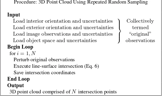
The actual construction of the 3D point cloud is accomplished by computing one 3D point at a time until a total ofN points are defined.Nis a large positive integer that denotes the number of RRS trials. At each trial the original unperturbed observables are perturbed according to the a priori stochastic model and a line-surface intersection algorithm (Eq. 6) returns the 3D object space coordinates of the intersection point. Figure 1 summarizes the process of generating the 3D point cloud.
The fidelity and spatial accuracy of RRS output point cloud is in-fluenced by several factors to include the fidelity of the a priori input stochastic error model (e.g., Gaussian, exponential, etc.), the quality of the pseudorandom number generator, and the num-ber of RRS trials executed. In practice, the quality of pseudo-random number generators is generally high, so the predominant factor influencing the accuracy of RRS output is the number of RRS trials executed.
function using the 3D point cloud itself. One way to build this empirical density function is to generate a voxel space surround-ing the point cloud and count the number of points that fall in each voxel. This realization of the empirical density function provides a framework where hypothesis testing can occur and is discussed later.
3.1 Size and Shape of Point Cloud
Several factors influence the size and shape of the the 3D point cloud generated by the RRS method. The factors fall into two separate categories: geometric factors and stochastic factors. The geometric factors include image collection geometry and terrain morphology, whereas the stochastic factors include a priori sto-chastic models and the nature of computational algorithms (deter-ministic or non-deter(deter-ministic). Finally, terrain interpolation falls in both categories. The contribution from each factor is described next.
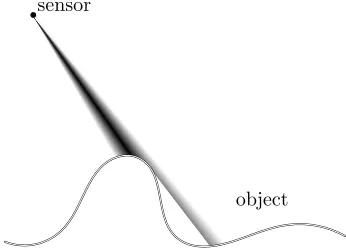
Geometry plays a large role in the resulting 3D point cloud. Con-ceptually, one can imagine a cone of uncertainty emanating from the sensor and projecting onto a surface with complex morphol-ogy. As image collection geometry changes from nadir perspec-tives to highly oblique perspecperspec-tives, the effect of object space occlusions can lead to discontinuities in the projected uncertain-ties (Figure 2). Depending on the circumstance — ranging from benign, smooth and continuous surfaces to urban surfaces with sharp corners — these discontinuities may lead to bi-modal or even multi-modal point clouds.
Stochastic factors also affect the resulting point cloud. For in-stance, if the a priori error covariance of the observations mapped to image space follows a multinormal distribution, then the “cone” of uncertainties will be conically shaped for uncorrelated image coordinates or elliptically shaped for correlated image coordi-nates. By contrast, if the a priori distribution is uniformly dis-tributed (i.e., a boxcar distribution), then the cone of uncertainty becomes more rectangular in shape. Separately, the nature of the computational algorithms that return the coordinates of the line-surface intersection may also affect the shape of the point cloud, especially if the algorithms are non-deterministic. Non-deterministic algorithms deliver a range of ouputs given a single input. The output from non-deterministic algorithms may contain random errors, systematic errors, or both.
Finally, surface interpolation methods fall into both the geomet-ric and stochastic categories. In a geometgeomet-ric sense, the interpo-lation method can introduce extreme discontinuities in the result-ing 3D point cloud when nearest neighbor interpolation methods are used, for instance. By contrast, a higher order interpolation method generally produces a smooth surface that may minimize the discontinuities in the resulting point cloud. From a stochas-tic perspective, surface interpolation may introduce both random and non-random errors into the resulting point cloud. The magni-tude of interpolation errors is a function of terrain point spacing, terrain morphology, and terrain interpolation method (Hu et al., 2009)
3.2 Special Case
The classical and RRS methods produce nearly identical esti-mates of uncertainty in at least one special case. This special case occurs when the a priori stochastic model is multinormal and when the object space is planar. The uncertainty estimate is realized in the form of a 3 by 3 covariance matrix that follows the multinormal distribution.
object sensor
Figure 2: A cone of uncertainty originates at the sensor and projects onto the object.
The reason the methods are only nearly identical and not exactly identical is because the classical method operates on a closed-form expression of the a priori stochastic model that completely describes the theoretical probability density function (PDF) as-sociated with the intersection point, whereas the RRS method attempts to closely approximate the theoretical PDF using a fi-nite number of empirical samples. The difference between the two methods tends to decrease as the number of RRS samples increases.
3.3 Hypothesis Test
The null hypothesis under evaluation is whether the coordinates of an intersection point,xI = [XI YI ZI]T, are consistent
with the coordinates of a truth point,xµ= [Xµ Yµ Zµ]T. As
in equation (3), the null and alternate hypotheses are stated as
Ho:xI−xµ=0
Ha:xI−xµ6=0 (7)
The objective of this test is no different than that of the classical method — to identify a density function and test statistic that are consistent with the null hypothesis. The primary challenge here is that the density function is unknown and must be created from empirical data points. Adding to the complexity, the density function is frequently non-Gaussian, potentially multi-modal in shape, and may contain random and non-random elements.
To meet these challenges and to accommodate the possibility of known a priori uncertainties in the truth point,xµ, an empirical
density function is constructed on the simple difference metric
d = xI−xµ. While other metrics could have been selected
and may be viable,dis selected here because it is rooted in the
null hypothesis statement and because it preserves the potentially complex shape and structure of the density function that origi-nates from the line-surface intersection. Like the classical case, when the a priori stochastic model is Gaussian and the object space is benign (i.e., planar), the expected value of dis zero.
However, in scenarios where the object space is complex, the den-sity function ofdcan become irregular, causing expected values
to differ from zero.
Procedure: 3D Point Cloud Using Repeated Random Sampling
Input
Load interior orientation and uncertainties Load exterior orientation and uncertainties Load image observations and uncertainties Load object space and uncertainties
Collectively termed “original” observations
Begin Loop fori= 1, N
Perturb original observations
Execute line-surface intersection (Eq. 6) Save intersection coordinates
End Loop Output
3D point cloud comprised ofNintersection points
Figure 1: Procedure to obtain empirical 3D point cloud using RRS method
ρdat an arbitrary voxel is computed as
ρd(i, j, k) =
Number of points in voxel
N
( 1≤i≤M
1≤j≤M
1≤k≤M
(8)
The outcome of this exercise is an expression – much like the analytical function in the classical case – whose total mass is 1 or
M X
i=1
M X
j=1
M X
k=1
ρd(i, j, k) = 1 . (9)
Given access to the individual voxel densities, the proposed ap-proach is to use standard elements of classical hypothesis testing as a guide with adaptations to accommodate the empirical na-ture of the problem and to accommodate the potentially complex shape and structure of the density function.
Thep-value is a classical element that is reused here; it serves as a computed quantity to determine if the null hypothesis is rejected or not. To obtain thep-value let the integers(ip, jp, kp)denote
the indices of the voxel containing the point
d= [XI−Xµ YI−Yµ ZI−Zµ]T. (10)
Then thep-value ,p, is computed as
p= X
(i,j,k)∈A
ρd(i, j, k) 0≤p≤1 (11)
whereAis the set of all indices(i, j, k)where the voxel density is less than or equal to the voxel density containing pointdor
A={(i, j, k) | ρd(i, j, k)≤ρd(ip, jp, kp)} (12)
Thep-value is small whendis inconsistent with the null
hypoth-esis and large whendis consistent with the null hypothesis. Let
αdenote the user-defined significance level of the test. The deci-sion rule is to reject the null hypothesis whenp < α.
The actual construction of the density function associated withd
is obtained by augmenting the steps used to obtain the RRS point cloud described in Figure 1 with additional steps to accommodate truth point uncertainty and to place the observed data points into a voxel space. When it exists, the truth point uncertainty inflates the geometric size ofρd. Let the origin of the density function lie
at a point xI nominal defined by the original, unperturbed
ob-servations. Also, in the context of theNRRS trials, let perturbed
Parameter value and standard deviation focal length = 100mm ± 0.01mm ximage coord. = 0mm ± 0.01mm yimage coord. = 0mm ± 0.01mm
XL = −500m ± 1m
YL = 40m ± 1m
ZL = 500m ± 1m
ω = 0◦
± 0.2◦ φ = −47.15◦
± 0.2◦
κ = 0◦ ± 0
.2◦ Table 1: Frame image parameters used in example
values be denoted with an elevated tilde (e.g.,˜xIdenotes the
per-turbed intersection point). Then the empirical data points that make up the density function are defined by three steps which are repeated at each trial: 1) perform the ray intersection using perturbed observations to obtain˜xI, 2) add a perturbation toxµ
according to the truth covariance matrixΣµµto obtainx˜µ, and
3) obtain a single datapointd˜ = ˜xI−x˜µ. TheN data points
obtained in this manner are then placed in the voxel space and the density function aboutdis computed. Figure 3 summarizes
these steps.
3.3.1 Example The theory above is applied to a real-world single-image example in this section. The data consist of a syn-thetic gridded elevation model and a synsyn-thetic image (Figures 4 and 5) to test whether the coordinates of an intersection point are consistent with the coordinates of an externally-defined ground truth point. Linear units are in meters and angular units are in decimal degrees. For simplicity it is assumed that all observables are normally distributed and uncorrelated. To simplify the exam-ple, the gridded elevation data is assumed to have no absolute or relative horizontal error (i.e.,σ = 0). By contrast the absolute elevation uncertainty at each node of the grid isσ =±1meter with no correlation between nodes. Bilinear interpolation is used to define terrain elevations between nodes. The elements of the standard frame image are described in Table 1. A total ofN = 100,000trials are used to describe the density function surround-ing xI nominal . The coordinates of the nominal intersection
point are computed using the nominal values appearing in Table 1 and Figure 4 to producexI nominal ≈[32.78 30.00 5.78]T
. The known, externally-derived truth point is defined with coor-dinatesxµ = [30.00 29.00 4.00]T with a covariance matrix
equal toI3. Consequently, the difference vector for this sample
data isd = xI−xµ ≈ [2.78 1.00 1.78]T. Voxels are 0.5
meters on a side.
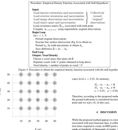
Procedure: Empirical Density Function Associated with Null Hypothesis
Input
Load interior orientation and uncertainties Load exterior orientation and uncertainties Load image observations and uncertainties Load object space and uncertainties
Collectively termed “original” observations
Load covariance matrixΣµµassociated with truth point
Compute xI nominal using unperturbed, original observations
Begin Loop fori= 1, N
Perturb original observations
Execute line-surface intersection (Eq. 6) to obtain˜xI
Perturbxµby truth uncertainty to obtainx˜µ
Save differenced˜= ˜xI−x˜µ
End Loop
Output: Voxel Density
Choose a voxel space that spans alld˜
Populate voxels withNpoints obtained in loop above Voxel density = number of points in voxel /N
Figure 3: Procedure to obtain the empirical density function associated with the null hypothesis
1
1
1 1
1
1
1 1
1
1
1 1
1
1
1 1
1
1
1 1
2 8 2
1 8 0
2 8 2
10 10
20 20
30 30
40 40
50 50
X(m)
Y
(
m
)
Figure 4: Synthetic terrain data defined by a grid of raster ele-vations. Elevation data are in meters and are provided in shaded circles.
Figure 5 illustrates the notional geometry of the problem as well as the location of 100 intersection points relative to the gridded elevation model. These intersection points are computed using the procedure outlined in Figure 1. A bimodal distribution of the RRS point cloud is evident in Figure 5 where one mode lies near the highest elevation in the elevation model and the second mode lies at the lower elevation beside it.
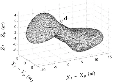
Given the object-space points in the RRS point cloud, the next step is to compute the density of each voxel using the proce-dure outlined in Figure 3. This voxel space is illustrated in Fig-ure 6 where an isosurface is rendered on the density function con-structed from the entire set ofN = 100,000points. As expected, Figures 5 and 6 exhibit a similar bi-modal distribution since they are produced from the same RRS simulation.
From a qualitative point of view, we reject the null hypothesis, Ho, because the pointdlies outside the1−α = 0.95
confi-dence surface; we would acceptHo ifdlied inside the surface
(Figure 6). From a quantitative perspective, the null hypothesis is rejected because thep-value ,p= 0.002, is less than the
signifi-cance levelα= 0.05. In summary,
Ho:xI−xµ=0
Ha:xI−xµ6=0
α= 0.05, p= 0.002
(13)
Therefore, according to this proposed methodology, sincep < α, the ground truth point is considered inconsistent with intersection point and werejectHoin this case.
4 DISCUSSION
While the proposed method appears to correctly handle challenges associated with non-Gaussian data, it suffers from long computa-tion times required to create an RRS point cloud containing thou-sands or hundreds of thouthou-sands of points. In the example it took neary 24 hours of computation time on a modern desktop com-puter using a crude 4-threaded parallel processing scheme.
Given today’s computing power it may be difficult to generate the RRS point cloud and compute the intersection uncertainty in near real-time. The computational task would be difficult even under ideal circumstances with highly-optimized multi-core and multi-threaded computational resources. The computational bur-den grows substantially when one imagines computing intersec-tion uncertainties for every pixel on an image.
5 CONCLUSIONS AND FUTURE
A repeated random sampling method has been proposed to char-acterize the spatial uncertainty at a point where a line intersects a surface. The classical method of characterizing spatial uncer-tainty is restricted to cases where the object surface is planar. The RRS method, on the other hand, makes no assumptions concern-ing surface morphology. The RRS method does not provide di-rect access to a closed-form expression of the probability density function; consequently an empirical density function is created from the 3D data points produced by the RRS method. The em-pirical density function is realized through a simple technique us-ing voxels.
X
RRS points denoted by circles
Figure 5: Synthetic data set illustrating notional geometry be-tween image and object. The 3D point cloud in object space is produced using a synthetic image and terrain data described in the text. The symbol⊗denotes the nominal location of the in-tersection point in the image and raster elevation model, while points in the RRS point cloud are denoted by “◦”. For visual clarity, the first 100 of theN = 100,000points are plotted. The shape and bi-modal structure of the point cloud closely resembles the density function in Figure 6.
ZI
Figure 6: Isosurface rendered on density function ofd. The
iso-surface encapsulates 95% of the mass of the density function. The symbol⊙denotes the discrete data point associated withdused
in the example. The density function is produced from empirical data points using the procedure outlined in Figure 3.
A formal hypothesis test is designed to determine whether an externally-defined point and its associated uncertainty is consis-tent with the intersection point and its uncertainty. An empirical density function is constructed from the RRS process and a test statistic is used to determine if the null hypothesis is rejected or accepted.
Future efforts will focus on techniques to improve and enhance the fidelity of the RRS empirical density function. While the voxel method described in this paper is intuitive, other sophisti-cated methods of density estimation may result in greater fidelity of the density function while at the same time requiring fewer RRS trials. Likewise, methods such as stratified sampling seek to exhaustively interrogate the sample space using fewer trials (Wikipedia, 2010). Also, computation time may be improved by using an intelligent convergence test to determine when the den-sity function has reached a steady state and does not benefit from additional RRS trials.
ACKNOWLEDGEMENTS
The author would like to thank Henry Theiss and two reviewers for their generous and helpful comments on this paper.
REFERENCES
Beekhuizen, J., Heuvelink, G. B. M., Biesemans, J. and Reusen, I., 2011. Effect of dem uncertainty on the positional accuracy of airborne imagery. IEEE Trans. on Geoscience and Remote Sensing 49(5), pp. 1567–1577.
Cuartero, A., Felicisimo, A. M., Polo, M. E., Caro, A. and Ro-driguez, P. G., 2010. Positional accuracy analysis of satellite imagery by circular statistics. Photogrammetric Engineering & Remote Sensing 76(11), pp. 1275–1286.
Hu, P., Liu, X. and Hu, H., 2009. Accuracy assessment of digital elevation models based on approximation theory. Photogrammet-ric Engineering & Remote Sensing 75(1), pp. 49–56.
Klein, J. and Zachmann, G., 2004. Point cloud collision detec-tion. Eurographics 23, pp. 567–576.
Mikhail, E. M. and Ackerman, F., 1976. Observations and Least Squares. University Press of America.
Mikhail, E. M., Bethel, J. S. and McGlone, J. C., 2001. Introduc-tion to Modern Photogrammetry. John Wiley & Sons, Inc., New York.
Mohamed, R., El-Baz, A. and Farag, A., 2005. Probability den-sity estimation using advanced support vector machines an the expectation maximization algorithm. World Academy of Science, Engineering and Technology.
Parzen, E., 1962. On estimation of a probability density function and mode. AMM. Math. Stat. 33, pp. 1065–1076.
Pollard, T., Eden, I., Mundy, J. and Cooper, D., 2010. A volumet-ric approach to change detection in satellite images. Photogram-metric Engineering & Remote Sensing 76(7), pp. 817–831.
Press, W., Vetterling, W., Teukolsky, S. and Flannery, B., 1988. Numerical Recipes in C. Cambridge University Press.
Wikipedia, 2010. Wikipedia 2010. http://en.wiki-pedia.org/wiki/Stratified sampling (last date accessed: 28 Sep 2010.).