A COMPARITIVE STUDY USING GEOMETRIC AND VERTICAL PROFILE
FEATURES DERIVED FROM AIRBORNE LIDAR FOR CLASSIFYING TREE GENERA
C. Ko1*, G. Sohn1 and T.K. Remmel2
1 Department of Earth & Space Science & Engineering, York University, Toronto, Ontario, Canada - (cko, gsohn)@yorku.ca 2 Department of Geography, York University, Toronto, Ontario, Canada - [email protected]
Commission III, WG II/2
KEY WORDS: LiDAR, tree genera, classification, Random Forest, feature selection, vertical profile
ABSTRACT:
We present a comparative study between two different approaches for tree genera classification using descriptors derived from tree geometry and those derived from the vertical profile analysis of LiDAR point data. The different methods provide two perspectives for processing LiDAR point clouds for tree genera identification. The geometric perspective analyzes individual tree crowns in relation to valuable information related to characteristics of clusters and line segments derived within crowns and overall tree shapes to highlight the spatial distribution of LiDAR points within the crown. Conversely, analyzing vertical profiles retrieves information about the point distributions with respect to height percentiles; this perspective emphasizes of the importance that point distributions at specific heights express, accommodating for the decreased point density with respect to depth of canopy penetration by LiDAR pulses. The targeted species include white birch, maple, oak, poplar, white pine and jack pine at a study site northeast of Sault Ste. Marie, Ontario, Canada.
1. INTRODUCTION
The goal of this paper is to compare the effectiveness of using geometric feature based descriptors for tree genera classification compared to the more conventional vertical profile descriptors. The advantages of deriving geometric descriptors are that these descriptors can be easily related to the physical and biological implication of tree form, such as growth direction, tree crown shape and the representation of internal tree crown structure. It also provides us with a graphical illustration of the tree for interpretation and an important visual aid for presentation. Conventional methods for retrieving vertical profile descriptors have proven effective and accurate for tree species classification. For example, Holmgren and Persson (2004) successfully classified Norway spruce and Scots pine with an overall classification accuracy of 95%; Moffiet et al. (2005) achieved an accuracy of 77% classifying Cypress Pine, Poplar Box, Silver Leaved Ironbark, Smooth Barked Apple and Brigalow; Ørka et al. (2007) achieved an accuracy of 74% for classifying spruce, birch and aspen. Ørka et al. (2009) achieved an accuracy of 88% for classifying large Norway spruce and birch trees. In the same year, Suratno et al. (2009) reported a classification accuracy of 95% when classifying ponderosa pine, Douglas-fir, western larch and lodgepole pine. Korpela et al. (2010) achieved an accuracy of up to 90% classifying Scots pine, Norway spruce and birch by using intensity variables; and Vauhkonen et al. (2010) showed a classification rate of 78% classifying Scot pine, Norway spruce and deciduous trees.
This paper investigates the results from two different approaches for tree species/genera classification, the first approach classifies tree genera by extracting geometric information from LiDAR point data, we derived 24 features for each tree crown, instead of looking at the point distribution within individual tree crowns using height percentiles, we derive geometric information to provide context to the
individual LiDAR tree crowns. The features are categorized into five groups:
1. Line related features – describe orientation and characteristics of line segments (hypothetical branches) derived from within the tree crown 2. Cluster related features – describe the shape of the
clusters derived from individual segmented tree crowns
3. Convex hull and alpha shape related features – describe the outer shape of the tree crowns
4. 3D buffering related features – describe the amount and characteristics of LiDAR point density inside a tree crown
5. Overall tree shape related features
The second approach classifies tree genera by extracting vertical height profile information from LiDAR points, we derived 78 features for each tree crown and the features can be categorized into three groups:
1. Percentage of first, single, and last returns at different height percentiles
2. Mean, standard deviation, coefficient of variation, kurtosis, skewness of first, single, and last returns for height values at different height percentiles
3. Mean, standard deviation, coefficient of variation, kurtosis, skewness of first, single, and last returns for intensity values at different height percentiles
We would like to study the potential to reduce the number of features for classification and the possibility to combine the most important features for classification. The advantage of combining features derived by two different methods is to take advantage of both perspectives, but before we can achieve this goal, we need to look at the features separately. The next step after this is to see if the two set of features are competitive or co-operative and combine them in a multiple classifier systems. Being able to classify tree genera or species accurately at a
stand level is useful for many applications. First, forest inventory can be updated more efficiently and therefore will have a better assessment for biomass estimation and a more effective forest management strategy. Another application related to this project is for identifying tree genera along utility transmission line right-of-ways (ROW); knowing tree genera information allows utility companies to better manage vegetation along the ROW. In conjunction with the growth and yield tables, managers can better estimate and predict the potential growth of the vegetation in or near the ROW. This can be used to determine the amount of tree cutting, trimming or pruning to maintain safe clearance zones.
2. STUDY AREA AND METHODS
2.1 Study area
The study area is located near Thessalon about 75 km east of Sault Ste. Marie, Ontario, Canada. We have selected eight field sites for capturing the diversity of environmental conditions in that region. In our study area, we have identified white birch (Betula papyrifera Marsh.), balsam fir (Abies balsamea (L.)), maple (Acer saccharum Marsh.), red oak (Quercus rubra L.), jack pine (Pinus banksiana Lamb.), poplar (Populus temuloides), white pine (Pinus strobus L.), white spruce (Picea glauca (Moench Voss)) and others during field visits. With the variety of species, our project aims to classify these species into three broader genera, pine, poplar, and maple. We sampled 186 trees during our field validation visit but only 160 of them belong to the genera of interest and therefore only those will be used for classification. The LiDAR data was collected on 7 August 2009, by a Riegl LMS-Q560 scanner. The flight altitude was about 122 m above ground level and the point density is approximately 40 pulses per m2 with up to five returns per pulse.
We have surveyed eight field sites and they are 1) Poplar1 with an approximate area of 0.56 ha. 2) Poplar2, 0.6 ha 3) Maple1, 1.7 ha, 4) Maple2 1.4 ha, 5) Maple3, 0.08 ha, 6) Corridor, 14.6 ha, 7) Pine1, 8.7 ha and 8) Pine2, 0.05 ha.
2.2 Methods
To classify the three genera, we have derived two sets of features and after the features are derived, we use Random Forest (Breiman, 2001) for classification and feature importance calculation.
Two field surveys were conducted from 30 July to 12 August 2009 and 8-10 August 2011. 18 trees were measured during the first field visit, attributes measured include tree height, tree crown base height, tree crown diameter and diameter at breast height (DBH), the center location of the 18 trees was measured by total station as well as a handheld GPS. LiDAR trees were isolated after visiting the field with the coordinates measured. During the second visit, only tree location (measured by handheld GPS), species and DBH are measured. Individual LiDAR trees were segmented manually before visiting the field site.
2.2.1 Features for classification: We derived features for classification in two different ways, the first involve defining groups of clusters within each tree crown, then the behaviours of best fit planes and lines for each cluster are described resulting features in F1 to F10 (Table 1). Volume and area related metrics for the tree crown are listed as F11 to F17 (Table 1).
The properties of how LiDAR points inside the tree crown conglomerate with the neighbouring LiDAR points if each point is buffered outward at a distance of 2% of the tree crown height is described by F18 to F21 (Table 1). The last category summarizes the overall tree shape (F22 to F 24). The detailed methodology of how each feature is calculated is described in Ko et al. (submitted). In total, we derive 24 features; each is described in Table 1.
No. Description Line related
F1 Average line segment lengths divided by tree height F2 Average line segment lengths divided by tree crown
height
F3 Average line segment lengths multiplied by the ratio between tree crown height and tree height
F4 Average line segment angles (rad) measured from the x-y plane to the line
F5 Average line segment angles (rad) measured from the y-axis to the line projected onto the x-y plane
Cluster related
F6 Average number of points in each cluster divided by the number of points in the tree crown
F7 Average of the average orthogonal distance from each point to the line in the tree crown for each cluster F8 Average of the average orthogonal distance from each
point to the plane in the tree crown for each cluster F9 F7 divided by the tree crown height multiplied by F8
divided by the tree crown height
F10 Average of the volume of the convex hull for each cluster divided by the number of points in the cluster Convex hull and alpha shape related
F11 Average of volume of the convex hull for each cluster divided by the number of points in the cluster
F12 The difference between the area of the convex hull and the alpha shape compared to the convex hull area F13 Volume of the tree crown convex hull divided by the
number of points in the crown
F14 Volume of the tree crown alpha shape divide number of points in the crown
F15 Average distance from each point to the closest facet of the convex hull
F16 Standard deviation of orthogonal distances from each point to the convex hull
F17 Coefficient of variation (F15/F16) 3D buffering related
F18 Sum of overlapped volume between ith and jth spheres F19 Overlapped count of points captured by ith and jth
spheres
F20 Overlapped volume divided by the number of points in the tree crown
F21 Number of count divided by the number of point in the tree crown, squared
Overall tree shape related
F22 Tree height divided by the radius of the tree crown, radius is obtained by assuming when the tree crown is projected to xy plane, it is circular
F23 Tree crown height divided by the radius of the tree crown, radius is obtained by assuming when the tree crown is projected to xy plane, it is circular
F24 Tree crown height divided by the tree height
Table 1. Descriptive summary of geometric derived features
The second set of features describes the vertical point distribution (height attributes and intensity attributes). There are 78 features for each tree derived. Table 2 summarizes these features. Each tree is height normalized and segmented into 10 vertical slices. The 10th percentile features represent the LiDAR points belonging to the bottom 10th percentile of the tree crown height whereas the 90th percentile features represents the points located at the top of the tree. Features include “first of many” returns; “single return” and “last of many” returns. Feature numbers are in bold.
V1 to V12 are attributes related to counting the percentage of points belonging to the first, single, or last category in different percentiles. V13 to V45 are features related to statistics of
V40. Kurtosis of variation height for first canopy return (V41. s) (V42. l)
V43. Skewness of variation height for first canopy return (V44. s) (V45. l) V73. Kurtosis of variation intensity of first canopy return
(V74. s) (V75. l)
V76. skewness of variation intensity of first canopy return (V77. s) (V78. l)
Table 2. Summary of features derived from vertical point profile: s= single; l= last; Std= standard deviation; Cv = coefficient of variation
Figure 1 shows an example of a sample tree from each genus we are trying to classify. Figure 1(a), (b), and (c) is an example of a pine, poplar and maple respectively and (d), (e), and (f) is an example of the point distribution for each genera, showing first of many returns, last of many returns, single returns and all return for pine, poplar and maple respectively
2.2.2 Random Forest: We use Random Forest for classification. Random Forest is an algorithm that construct a numerous classification trees recursively by randomly selected variables (Breiman, 2001), in our case, using the core randomForest package of the R software. This is a process for training the classification tree, Random Forest internally partitions approximately of the data for tree construction and use the remaining of the data for validation, called out of bag data (OOB). Therefore, the OOB error calculated from Random Forest represents the training error. In each of the iteration, different sub set of the features will be selected randomly for constructing the classification tree. By replacing different features, each iteration will result in different OOB error, the change of the error therefore determines whether a particular feature improve or degrade the overall classification and the change is recorded (mean decrease permutation accuracy) to evaluate the importance of the particular feature.
We did not use the default OOB error for evaluating our classification results because in forestry applications, situations that allow using of the data for training are rare. Moreover, we would like to find the optimal amount (least required for training and yet producing reasonable classification accuracy) of data required for training the Random Forest classifier.
(d) (e) (f) (a) (b) (c)
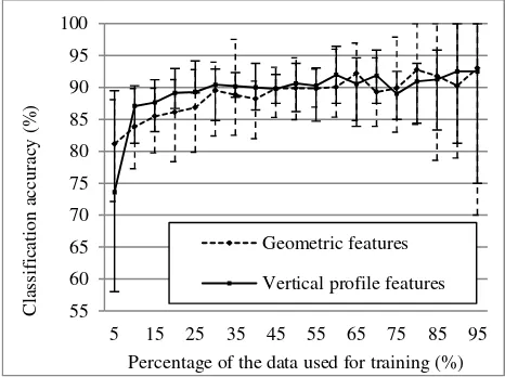
Therefore we performed an additional test; the test will investigate the sensitivity of classification accuracy with incremental increase (5%) training data. Start from using 5% of the entire dataset for training (95% for validation), Random Forest and validation are repeated 20 times and the average OOB and classification accuracy (obtained from partitioned validation dataset) are obtained. The average classification for both sets of features are plotted in Figure 2.
3. RESULTS
3.1 Partitioning results
The classification accuracy increases for both sets of features when the data partitioned for training increases because there are more referenced data for training the classifier; the variance of classification accuracy decreases as the proportion of training data increases for the same reason. However, when the training partition approaches or exceeds 85%, the validation data becomes relatively small and thus a single mis-classified sample will lead to a large reduction in classification accuracy, resulting in a large variance when the validation sample size diminishes. The classification accuracy in Figure 2 represents the mean accuracy obtained from running Random Forest 20 times at each partitioning increment. The error bars shown in Figure 2 represents the minimum and maximum classification accuracy obtained within the 20 trials. At each trial, it is a balanced sample selection meaning we made sure each training set had similar amount of pine, maple and poplar in each partition. For both sets of features, by only using 5% of the data for training, the classification accuracy can reach an average of 77%. From 10% to 25%, vertical profile derived features have a higher rate of gaining accuracy whereas geometric derived feature classifications increase at a slower rate until the 30%
Percentage of the data used for training (%) Geometric features
Vertical profile features
Figure 2. The average change in classification accuracy with increasing percentage of the data used for constructing classification trees, upper bars and lower bars represents the maximum and minimum accuracy respectively
3.2 Classification accuracy
In section 3.1, we show that for this project, by using 30% of the data for running training is optimal. Both methods can achieve comparable classification accuracy. Table 3 and Table 4 show the confusion matrices for classification by geometric derived features and vertical profile derived features at a 30%
Table 3. Confusion matrix for the classification accuracy averaged over 20 iterations using 30% of the data for training
Table 4. Confusion matrix for the classification accuracy averaged over 20 iterations using 30% of the data for training using vertical profile derived features (values are average over 20 iterations)
We used 70% of the 160 trees for validation; when this process is repeated 20 times with different samples, this result in 2240 trees. The overall accuracy for both methods is 90% and both methods exhibit lowest class error when classifying maple trees and both sets of features have highest class error classifying poplar trees.
3.3 Feature importance
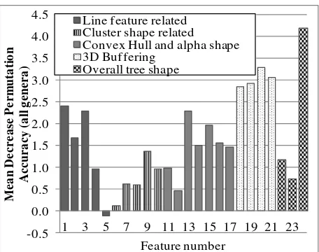
Feature importance is calculated by the mean decrease permutation accuracy. When running Random Forest, OOB error that is being recorded from each tree, e. Then, for each feature, fk, where k = number of features, the randomly permuted kth feature is being used and therefore will produce a new OOB error ek. Importance can be measured by using ek– e, average over all trees and are normalized by the standard deviation. This is called “mean decrease permutation accuracy” and is used in this paper. If a feature has a large value that means it is more important for classifying the three shapes and vice versa. Figure 3 shows the feature importance graph for geometric derived features and Figure 4 shows the feature importance graph for vertical profile derived features.
-0.5 genera for geometric derived features using 30% of the data for training genera for vertical profile derived features
Figure 3 shows that the two most important features derived from geometric attributes are F24 and F20; where F24 represents the ratio between the tree crown height and the tree height. F20 is calculated by buffering all LiDAR points outward by a distance equal to 2% of the tree crown height, points that increasingly proximal will result an overlapping volume. F20 therefore is the summation of all overlapping volumes from all possible points divided by the total number of LiDAR points within the tree crown.
Figure 4 shows that the two most important features derived from vertical profile attributes are V11 and V44; where V11 represents the percentage of single returns at 90th percentile, and V44 is the skewness of variation in height for the canopy, single return only.
4. DISCUSSION AND CONCLUSION
From Figure 2, we show that the OOB error rate is not the only way to evaluate classification accuracy and stability, instead of using of the entire dataset for constructing the classification tree, we have chosen to use 30% of the data for running
Random Forest. We also showed that both sets of features show a very similar rate of increase in classification accuracy when the training sample size increases. Models that are built by the two sets of features learn at a similar pace. The error bars for both methods are large when the training sample sizes are small because if the sample being selected for training is not representative of the trees in the area, then the classification accuracy could be very low. The error bars are also large when the testing sample sizes gets smaller because one misclassified tree can result in a significant reduction in the classification accuracy.
The overall accuracies for both methods are the same (90%) when using 30% of the data for training and 70% of the data for testing. Both features have the greatest difficulty differentiating between pines and poplar. This is because the vertical point distribution between pine and poplar are similar, with points located mostly at the top of the tree crown, density reduces, into the tree crown and decreases dramatically after it reaches the bottom of the tree crown (Figure 1d and 1e), where only points from the tree trunks are returned to the scanner. From the geometric feature perspective, the ratio between the tree crown and tree height for both genera could sometimes be similar resulting in the confusion. Geometric based features are more accurate in predicting pine trees and the error mostly comes from mistaking pine trees as poplars. Conversely, vertical profile derived features are more accurately classifying poplar trees. Both methods have high class accuracy for maple because maple trees usually grows in closed canopies where LiDAR pulses rarely reach to the lower levels of the forest canopy, resulting a sharp decrease in point density with height in the top part of the tree crown which is different from pine and poplar. The densely growing understory associated with maple field sites also makes the detection of the tree crown base difficult, often detected very close to the ground level (minimum height recorded from the LiDAR points for a particular segmented single tree). Lines (branches) derived from maple trees tend to be shorter and located at the top of the tree with no obvious orientation. As mentioned, the LiDAR points are mostly located at the top of the tree crown due to the low penetration rate, when points are buffered outward, the volume of overlapping also increases for maple trees compared with poplar trees.
The two most important geometric features are the ratio between the tree crown height and the tree height (F24); and the overlapping volume by the buffered spheres divided by the number of points within the tree (F20). Poplars have the smallest ratio (small size tree crown) whereas maples have the largest. In the case where the bottom of the tree crown base cannot be detected, the ratio is equal to one. F20 highlights the tree crown spatial distribution properties among the genera, pines and maples have high values because points tends to (V11) and skewness of variation in height for the canopy, first return only (V44). V11 is related to the penetration rate, it is noted that, at 90th percentile, if a tree permits LiDAR pulses to penetrate further into the tree crown, the proportion of single return is less, for example in Figure 1d, pine tree leaves are smaller than poplar (Figure 1e) and maple (Figure 1f). As a result, the proportions of single returns for poplar and pine trees are higher at 90th percentile. For the same reason, V44 is the
skewness of height distribution for single returns and is also important in differentiating the three genera.
Our vertical profile feature research demonstrates similar results with Persson and Holmgren (2004), where the important features located in the upper percentiles of the tree top. We also show that height attributes and the count attributes are more important than the intensity attributes, this is unlike the studies found in Korpela et al. (2010) but their intensity values are normalized by range and ours are not. Intensity values should be normalized by range because it is a function of range itself and to be able to interpret the received intensity value properly, the effect of range has to be removed. In Ørka et al. (2009), by using uncalibrated intensity value, they have shown that the maximum and mean intensity for first return and mean intensity for the last return are important for differentiating species for large trees. Our results illustrate that within the intensity attributes, V48 (mean intensity at the 10th percentile, last return only) is the most important feature.
Our comparative study shows that by using the two sets of features separately for classification, the classification accuracies are about the same. We also confirm the possibility of using geometric derived features for classification. The advantage of using geometric derived features is their valuable association between the derived geometric features within the tree crown to the actual tree forms. Although the classification accuracies are very similar in our studies, we believe the two sets of the features should complement each other under complex environmental conditions. For example, when tree crowns are severely overlapped with each other, or when only half the tree can be viewed by the LiDAR scanner, this situation is common in ROW corridor applications, due to the required vegetation clearance zones along both sides of the infrastructure; one side of the tree can be viewed openly whereas the other side of the tree could be occluded by other vegetation. We have already noted that there are some discrepancies in class error, meaning some features in each set of features are better at classifying certain genera. We also would like to discover if the performance of the two sets of features behave differently in complex situations.
5. ACKNOWLEDGEMENT
This research was funded by GeoDigital International Inc., Ontario Centre for Excellence (OCE) and NSERC.
6. REFERENCE
Breiman, L., 2001. Random forests. Machine Learning, 45(1), pp. 5-32.
Holmgren, J., and Å Persson, 2004. Identifying species of individual trees using airborne laser scanning. Remote Sensing of Environment, 90(4), pp. 415-423.
Ko, C., G. Sohn and T.K., Remmel, (submitted). Tree form classification with geometric features from high-density airborne LiDAR. Photogrammetric Engineering & Remote Sensing.
Korpela, I., Ørka, H. O., Maltamo, M. and Tokola, T., 2010. Tree species classification using airborne LiDAR—Effects of stand and tree parameters, downsizing of training set, intensity normalization and sensor type. Silva Fennica, 44(2), pp. 319– 339.
Moffiet, T., Mengersen, K., Witte, C., King, R. and Denham, R., 2005. Airborne laser scanning: exploratory data analysis indicates potential variables for classification of individual trees or forest stands according to species. ISPRS Journal of Photogrammetry and Remote Sensing, 59, pp. 289–309.
Ørka, H.O., Næsset, E. and Bollandsås, O.M., 2007. Utilizing airborne laser intensity for tree species classification. International Archives of the Photogrammetry, Remote Sensing and Spatial Information Sciences, 36, pp. 300–304 Part 3/W52.
Ørka, H.O., Næsset, E. and Bollandsås, O.M., 2009. Classifying species of individual trees by intensity and structure features derived from airborne laser scanner data. Remote Sensing of Environment, 113(6), pp. 1163-1174.
Suratno, A., Seielstad, C. and Queen, L., 2009. Tree species identification in mixed coniferous forest using airborne laser scanning. ISPRS Journal of Photogrammetry and Remote Sensing, 64(6), pp. 683-693.
Vauhkonen, J., Korpela, I., Maltamo, M. and Tokola, T. 2010. Imputation of single-tree attributes using airborne laser scanning-based height, intensity and alpha shape metrics. Remote Sensing of Environment, 114(6), pp. 1263–1276.