Buying several indivisible goods
a ,* b c
´ ´
Carmen Bevia , Martine Quinzii , Jose A. Silva a
` ` `
Departament d’Economia i d’Historia Economica, Universitat Autonoma de Barcelona, 08193 Bellaterra, Barcelona, Spain
b
Economics Department, University of California, Davis, CA, USA c
Universidad de Alicante, Alicante, Spain
Received 4 August 1997; received in revised form 17 December 1997; accepted 6 February 1998
Abstract
This paper studies economies in which agents exchange indivisible goods and money. The indivisible goods are differentiated and agents have potential use for all of them. We assume that agents have quasi-linear utilities in money, have sufficient money endowments to afford any group of objects priced below their reservation values, have reservation values which are submodular and satisfy the cardinality condition. This cardinality condition requires that for each agent the marginal utility of an object depends only on the number of objects to which it is added, not on their characteristics. Under these assumptions, we show that the set of competitive equilibrium prices is a non-empty lattice and that, in any equilibrium, the price of an object is between the social value of the object and its value in its second best use. 1999 Elsevier Science B.V. All rights reserved.
Keywords: Indivisible goods; Cardinality condition; Agents; Money
1. Introduction
This paper considers economies in which agents can buy and sell indivisible goods and in which all payments are made in units of a divisible good that, following standard use, we call money. This model is probably closer to many circumstances of exchange in the real world than the standard model in which all goods are assumed to be perfectly divisible, but is also more difficult to analyze. The use of marginal calculus is precluded, and the application of fixed point theorems based on continuity properties, still possible in some cases, is certainly not straightforward. In consequence the model has been studied under restrictive assumptions, which are progressively being relaxed. Until
*Corresponding author. E-mail: [email protected]
recently it was assumed either that all the indivisible goods were all units of the same good (Henry, 1970), or that buyers had use only for one type of indivisible good (Kaneko and Yamamoto, 1986), or just for one of the indivisible goods: this case covers most of the literature on assignment games and matching models (see Roth and Sotomayor (1990) for a comprehensive account of the results) and competitive equilibria of economies with indivisibilities (Kaneko, 1982; Gale, 1984; Quinzii, 1984). Recently several papers (Gul and Stacchetti, 1996; Bikhchandani and Mamer, 1997; Laan et al., 1997) have relaxed this assumption, and assumed that agents have use for several units of the indivisible goods, units which may be differentiated.
With the exception of Bikhchandani and Mamer (1997) who show that, if there are two types of agents with quasilinear utilities such that all agents of the same type have the same supermodular and increasing reservation values, a competitive equilibrium exists, all the results of these papers follow from assumptions of the agents’ demand functions rather than on their utility functions. Laan et al. (1997) impose a condition on agents’ demands which does not require quasi-linearity in money but seems to require separability of the utility functions with respect to the indivisible goods, while Gul and Stacchetti impose that the utilities be quasi-linear in money and that the demands satisfy the property of gross substitutability (to be formally defined in Section 2) introduced by Kelso and Crawford (1982) for a two-sided matching model between firms and workers. In contrast, this paper studies a class of economies which is defined by restrictions on the agents’ utility functions. First, the utilities are quasi-linear in money so that the preferences can be represented by reservation values for subsets of the available indivisible objects. Second, these reservation values are submodular i.e. the marginal utility of an object decreases when the set of objects to which it is added becomes larger. Last and not the least, this marginal utility depends only on the number of objects and not on the composition of the set to which it is added.
This last assumption, that we call the cardinality condition, is certainly strong. At the moment however, it is the only interpretable condition that we have found which precludes that, for at least one agent, some objects ‘fit’ better together than when they are associated with other objects — a situation which seems to cause non-existence of an equilibrium even with decreasing marginal utilities (see the example of non-existence in Section 2 or the one in Gul and Stacchetti (1996)). Under the assumption that utilities are submodular and satisfy the cardinality condition we show that the set of equilibrium
M
prices is non-empty, is a convex complete lattice and thus admits a vector p of maximum and a vector p of minimum equilibrium prices. Moreover these prices have am
M
natural economic interpretation: the maximum price p (a) of an object a is the contribution of this object to the social welfare, or its social value, while its minimum price p (ma) is its value in its second best use (these notions are precisely defined in Section 3).
those of Gul and Stacchetti. Being based on the study of the efficient assignments of the objects, they uncover properties of these efficient assignments which are of interest in themselves, and may be used to obtain results of comparative statics for this class of economy (see in particular Lemma 3.3 which describes some regularities of the efficient assignments when new objects are added to the available objects).
The paper is organized as follows: the model and an example of non-existence of equilibrium motivating the cardinality condition is presented in Section 2. The characterization of the prices supporting the efficient assignments of economies with submodular utility functions satisfying the cardinality condition is the subject of Section 3. Section 4 discusses the relation between the cardinality condition and the property of gross substitutability of demands.
2. The model
Consider an exchange economy e with a finite set I of agents (whose elements are denoted by i, j, . . . ), a finite setVof indivisible objects (whose elements are denoted by a,b, . . . ), and a perfectly divisible good called money. Agents’ preferences are quasi-linear: the utility that agent i[I derives from consuming a set of objects A can be
characterized by a reservation value V(i,A) which represents the quantity of money that agent i is ready to sacrifice in order to consume the objects in A. The utility of agent i holding m units of money and the set A of objects is thusi
u (A,m )i i 5V(i,A)1mi
For all i[I, the reservation value function V(i,.), defined on the power set P(V), is assumed to be weakly increasing (V(i,A)#V(i,B ) whenever A,B ) and to satisfy V(i,[)50.
¯ ¯ ¯ ¯
Agents’ endowments, (A ,m )i i i[I, with mi$0 and
<
i[IAi5V, are assumed to be¯
such that mi$V(i,V) for all i[I. This assumption implies that whenever the price of a
set A of objects is less than the reservation value V(i,A), agent i can afford to buy the objects in A.
Let ´denote the set of economies satisfying the above conditions. For an economy
e[´ an assignments of objects to agents is thus a partition of the objects among the agents. Let S(I,V) denote all possible assignments. A feasible allocation of e is a pair
uIu
¯
(s,m)[S(I,V)3R1 such that omi5om .i i[I i[I
the feasible allocations associated to the assignments which maximize the sum of the agents’ reservation values. Such an assignments, satisfying
O
V(i,s(i ))$O
V(i,t(i )), ;t[S(I,V),i[I i[I
is called an efficient assignment.
Suppose that the objects are exchanged on a market at prices ( p(a))a[V (prices are expressed in units of money). If agent i buys the set A of objects he will pay p(A)5 o p(a). The demand of objects D(i, p) of agent i at the price vector p5( p(a))a[V is a[A
defined by
D(i, p)5hA[P(V)uV(i,A)2p(A)$V(i,B )2p(B ), ;B[P(V)j
¯ ¯
The demand of agent i for money is then mi5mi1p(A )i 2p(A). This number is
always non-negative since, for A[D(i, p), V(i,A)2p(A)$0 (the empty set is always a
¯
possible choice), and since by assumption mi$V(i,V). The price vector p is a competitive equilibrium price vector if, for each i[I, there exists Ai[D(i, p) such that
the map i→Ai is an assignment. By Walras Law, this condition, which ensures equilibrium on the market for the indivisible goods, implies that the market for money is also in equilibrium. Thus a competitive equilibrium for the economy e can be defined as
uVu
a pair (s, p)[S(I,V)3R1 such thats(i )[D(i, p) for all i[I. It is easy to check that, if
(s, p) is a competitive equilibrium, then s is an efficient assignment. We say that an
uVu
efficient assignment s is supported by a price vector p[R1 if (s, p) is a competitive equilibrium.
Proposition 2.1. An economy e[´has a competitive equilibrium if and only if every efficient assignment s of e can be supported by a price vector.
Proof. If (s, p) is a competitive equilibrium, by definitionsis supported by p. Suppose that t is another efficient assignment. Then
V(i,s(i ))2p(s(i ))$V(i,t(i ))2p(t(i )), ;i[I.
The pair (t, p) is not an equilibrium if at least one of the inequalities is strict. But then, summing the inequalities leads to
O
V(i,s(i ))2p(V).O
V(i,t(i ))2p(V)i[I i[I
which contradicts thatt is efficient. Thus (t, p) is an equilibrium.
There exists a competitive equilibrium if and only if there is at least one efficient assignment supported by a price vector. By the above reasoning, this holds if and only if every efficient assignment is supported by a price vector. h
in the quasi-linear case that we are considering, if the reservation value functions are additive (V(i,A)5 o V(i,a)). In this case it is efficient to give each object to the agent
a[V
which values it most, and the price vector p such that p(a)5maxi[IV(i,a) supports such an assignment. In general an equilibrium may not exist (Henry, 1970; Bikhchandani and Mamer, 1997) and additional restrictions must be placed on the reservation value functions.
A condition that seems particularly attractive since it expresses, in the case of indivisible goods, the idea that the marginal utility of an additional item decreases when the bundle of goods to which it is added gets larger, is the assumption of submodularity.
Definition 2.2. A reservation value function is said to be submodular if it is satisfied for
all A,B in P(V)
V(i,A<B )#V(i,A)1V(i,B )2V(i,A>B )
or equivalently
V(i,A)2V(i,A•a)#V(i,B )2V(i,B•a), for alla[B#A
Under submodular reservation value functions, the existence of an equilibrium is guaranteed if all objects are identical (V(i,A)5V(i,uAu)) (Henry, 1970). But unfortunately, the assumption of submodularity is not sufficient to imply existence of an equilibrium for the case where the indivisible objects are not perfect substitutes for one another, as shown by the following example.
Example 1. Let e[´be such that I5h1,2,3j,V5ha,b,gj. The submodular reservation values of the agents for the different subsets of objects are given in Table 1.
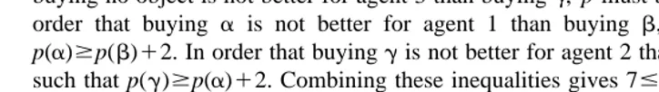
The only efficient assignment s of objects in this economy is such that s(1)5b, s(2)5a,s(3)5g. Suppose that p supports this assignment. In order that buyinghabjis not better for agent 2 than buying only a, p must be such that p(b)$5. In order that buying no object is not better for agent 3 than buyingg, p must be such that p(g)#8. In order that buying a is not better for agent 1 than buying b, p must be such that
p(a)$p(b)12. In order that buyinggis not better for agent 2 than buyinga, p must be such that p(g)$p(a)12. Combining these inequalities gives 7#21p(b)#p(a)#p(g)2 2#6, which is impossible.
Submodularity of the reservation values still permits complicated interdependence in utility among objects, which may prevent the existence of an equilibrium. In the previous example, if agent 2 has objectsaandb, then the marginal contribution ofais
Table 1
Non-existence with submodular reservation values
V \A a b g ab ag bg abg
V(1,A) 10 8 2 13 11 9 14
V(2,A) 8 5 10 13 14 13 15
equal to its value V(2,a) since V(2,ab)2V(2,b)51325585V(2,a), while if objectsa and g are combined the marginal contribution ofa is much lower: V(2,ag)2V(2,g)5 14210,V(2,a). Thus, for agent 2, having object bat the same time does not subtract any of the value ofa while having g lowers the desirability ofa.
A sufficient condition which ensures that the interdependence among objects is weak and that guarantees the existence of an equilibrium is that the demands of all agents satisfy the Gross Substitute (GS) assumption introduced by Kelso and Crawford (1982). Heuristically the demand of agent i satisfies the GS condition if, when the price of an object — let us say b — increases while the prices of all other objects stay the same, then the objects other thanbwhich were demanded by agent i are still demanded by this agent. This implies that there is no object which was demanded by agent i because it ‘fitted’ especially well withb, but is no longer desirable whenbbecomes too expensive. To state the formal definition of the GS property, let us adopt the following convention: we say that the objecta is in the demand of agent i at prices p if it belongs to at least one subset of objects demanded by agent i at p.
a[D(i, p)⇔a[A for some A[D(i, p)
Definition 2.3. The demand of agent i satisfies the gross substitute property if for any
uVu uVu
˜ ˜ ˜
p[R , and any p[R , p$p, with p(a)5p(a) for some a[V, then a[D(i, p) ˜
implies a[D(i,p ).
The gross substitute property however is not a condition on the primitive characteris-tics of the economy (the utility functions V(i,?)) but a condition on the derived demand functions (or more accurately demand correspondences). In this paper we will study a condition in the same spirit, which is stronger, but is made directly on the utility functions. The ‘cardinality condition’ that we impose requires that the marginal contribution of an object only depends on the number of objects to which it is added. This condition prevents interactions in utilities among objects — like objectsa and b fitting especially well together — which create problems for the existence of equilib-rium.
Definition 2.4. The utility function V(i,?) satisfies the cardinality condition if the marginal contribution of an object to agent i’s utility depends only on the number of objects to which it is added, i.e. for all A,B[P(V) such thatuAu5uBu and a[A>B
V(i,A)2V(i,A•a)5V(i,B )2V(i,B•a)
objects which are all of the same nature. The model studied in this paper generalizes, in the quasi-linear case the two-good model studied by Henry (1970) to the case where the indivisible objects are differentiated. An example of such objects could be paintings — or more generally art objects — collected by agents for purpose of decoration. The objects typically have different ‘esthetic values’ for different agents, and if the agents are more sensitive to the effect of each object than to the general effect that a group of objects produce together, then the cardinality condition can be a reasonable approxi-mation. The assumption that the agents’ reservation values are submodular seems also reasonable in this case, unless some agents are obsessive collectors.
The characterization of the cardinality condition given by the next proposition reveals that this condition is close to additive preferences. It simply adds to the valuation function a term of relative ‘satiation’ when several objects are consumed simultaneously.
Proposition 2.5. A reservation value function V satisfies the cardinality condition if and
only if there exists an increasing function f such that
V(A)5
O
V(a)2f(n), where n5uAu, f(0)5f(1)50 a[AIf in addition, V is submodular then f is supermodular i.e. f(n11)2f(n)$f(n)2f(n2 1) for all n.
Proof. It is clear that if the function V is as in Proposition 2.5 it satisfies the cardinality
condition. Let us prove the converse by induction on the cardinality of A. For any subset
A of V withuAu$2, define
f(A)5V(A)2
O
V(a) a[ALet A and B be two subsets of V such that A±B and uAu5uBu52. Let A5ha,a9j,
a[⁄ B, B5hb,b9j, b[⁄ A. Let C5ha,bj. By the cardinality condition, V(A)2V(A•a)5
V(C )2V(C•a) and V(B )2V(B•b)5V(C )2V(C•b). This is equivalent to V(A)2
V(a9)5V(C )2V(b) and V(B )2V(b9)5V(C )2V(a). Subtracting these two equalities gives f(A)5f(B ). Thus f takes the same value on all two-object subsets, value that we
denote f(2). Assume that for all values up to k, if A and B have the same number of elements which is less or equal to k, then f(A)5f(B ). Let us show that then this holds for k11. Let A,B[P(V) be such that uAu5uBu5k11. Suppose that A>B±[, and let
a[A>B. By the cardinality condition V(A)2V(A•a)5V(B )2V(B•a) which is equivalent to f(A)1V(a)2f(A•a)5f(B )1V(a)2f(B•a). This implies that f(A)5f(B )
since by the induction hypothesis f(A•a)5f(B•a). Suppose now that A>B5[. Let a[A,b[B and let D5A•a<b. ThenuAu5uDu5uBuand A>D±[, B>D±[. Using twice the previous argument leads to f(A)5f(B ). Thus f depends only on the cardinality
of the subsets. Let us show that if V is submodular then f is supermodular. Takea[V,
A and B two subsets such thatuAu5n21,uBu5n,a[⁄ A,a[⁄ B (for a feasible value of n). Then by submodularity V(A<a)2V(A)$V(B<a)2V(B ) which implies that f(n)2f(n2 1)$f(n11)2f(n). h
indivisible items related to their line of business (drilling permits, broadcasting permits, . . . ). In this case, assuming the cardinality condition means that the items do not present synergy in the production process. Adding submodularity implies that the marginal cost of some joint inputs (e.g. financing or management) increases with the number of items purchased. In the context of firms, the assumption that V is
1
supermodular — so that there are increasing returns to scale — is sometimes more appropriate than the assumption of submodularity. Unfortunately the following example shows that the existence of an equilibrium is not guaranteed if the agents’ reservation
2
functions are supermodular, even if they satisfy the cardinality condition.
Example 2. Let e[´ such that I5h1,2,3j, V5ha,b,gj. The reservation values of the agents for the different subsets of objects are given in Table 2.
The assignments s, s9, s0, s90 defined by: s(1)5habj, s(2)5hgj, s(3)5h[j; s9(1)5haj, s9(2)5hbgj, s9(3)5h[j; s0(1)5hbj, s0(2)5h[j, s0(3)5hagj; s90(1)5 h[j,s90(2)5hbj,s90(3)5hagjare efficient assignments. By Proposition 2.1, if there is a competitive equilibrium all these assignments must be supported by the same price vector p. Therefore a competitive price vector should satisfy,
V(1,ab)2p(a)2p(b)5V(1,a)2p(a)5V(1,b)2p(b)5V(1,[)
which is equivalent to
102p(a)2p(b)542p(a)542p(b)50
which is impossible.
In the following section we prove that if the utility functions are submodular and satisfy the cardinality condition, the set of equilibrium prices is non-empty and has the
M
lattice property found in the matching models with quasi-linear utilities. Thus if p (a) is the maximum value of object a for any equilibrium and p (ma) its lowest value in any
M M
equilibrium, then the vectors p and p are also equilibrium prices. Of course pm is the vector of equilibrium prices which is the most favorable for the sellers and p the mostm
M
favorable for the buyers. Moreover the prices p and pm have a natural economic
M
interpretation: p (a) is the social surplus created by objecta(to be precisely defined in Section 3) while p (m a) is the value of a in its second best use (also to be defined in
Table 2
Non-existence with supermodular reservation values satisfying the cardinality condition
V \A a b g ab g bg abg
V(1,A) 4 4 0 10 6 6 13
V(2,A) 0 4 4 6 6 10 13
V(3,A) 4 0 4 6 10 6 13
1
i.e. the inequality in Definition 2.2 is reversed. 2
Section 3). The analysis follows the route of the second Theorem of Welfare economics
M m
and shows that the prices p and p as well as a convex, complete lattice of intermediate prices support the efficient allocations of the objects among the agents.
3. Equilibrium prices
M
3.1. Definition of p and pm
The analysis of this section is made under the following set of assumptions on the utility functions which will not be repeated.
Assumption SC. For all i[I, the utility function V(i,?) is submodular and satisfies the cardinality condition.
Let s be an efficient assignment of the objects V to the I agents. The goal of this section is to derive the prices supporting this allocation of the objects. In a model with divisible goods and quasi-linear utilities, the prices supporting a Pareto optimal allocation are given by the multipliers associated to the scarcity constraints in the program of maximization of the sum of the utilities (social welfare) subject to the feasibility constraints. The envelope theorem then permits interpreting the multiplier associated to the scarcity constraint for a good (let us say gooda) as the change in social welfare resulting from a marginal decrease or increase in the supply of this good. Suppose now that good a is indivisible and exists in a single unit. If we proceed by analogy, there are two changes in the supply of a which play the role of a marginal change in the supply of a when the good is divisible: the supply can be decreased by one unit by taking the goodaout of the available supply of goods; or the supply can be increased by one unit by adding a copy of a to the supply of available goods. These changes induce changes in social welfare analogous to the changes in social welfare accompanying a marginal change in the supply of a divisible good. We will prove that these changes in social welfare define the maximum and minimum prices supporting the efficient allocation s.
Let us thus define the social welfare created by a supply Vof objects by
U(V)8
O
V(i,s(i )), for any efficient assignmentsofVi[I
M
Define p as the change in social welfare when the object a is taken out of the available objects, i.e.
M
p (a)5U(V)2U(V•a), a[V
or alternatively as the contribution of a to the social welfare. To define the minimum
˜
prices, for alla[Vleta denote an exact copy of objecta. To define the social welfare
˜
associated toV<a, we need either to extend the agents’ reservation value functions to
˜ ˜
subsets containing botha anda or to restrict ourselves to assignments ofV<a which
˜
assignaanda to different agents. We choose the second solution and define the set of
˜ ˜
˜ ˜
associated to V<a is then defined by
˜ ˜
U(V<a)5max
H
O
V(i,r(i ))ur[S 9(I,V<a)J
i[I
˜
and a solution to the maximum problem is called an efficient allocation ofV<a. The
˜
definition ofS9(I,V<a) is chosen in order to make it possible to consider assignments which allocate the object a to the agent i who has it in an efficient assignment of V, while giving a copy ofato the agent who would most benefit fromaafter agent i. Thus if we define
˜
p (m a)5U(V<a)2U(V), a[V
we can interpret p (ma) as the social value ofain its second best use (see Remark 1 after Lemma 3.3).
M M M
Define p 5( p (a))a[Vand pm5( p (m a))a[V. We first show that p (a) and p (ma) give respectively the highest and lowest possible equilibrium prices for object a.
Proposition 3.1. Let s be an efficient assignment of V, and suppose that there exists
uVu
˜
p[R1 supporting the assignment s. Then for all a[V, U(V<a)2U(V)#p(a)#
U(V)2U(V•a).
Proof. Since the vector p is supporting the assignment s, for all i[I, and for all A[P(V), V(i,s(i ))2p(s(i ))$V(i,A)2p(A). In particular, given a[V, let t be an
˜
efficient assignment ofV•aamong I, and letrbe an efficient assignment ofV<a. As noted above, assume w.l.o.g. thatr(i )[Vfor all i. Then, V(i,s(i ))2p(s(i ))$V(i,t(i ))2
p(t(i )) and V(i,s(i ))2p(s(i ))$V(i,r(i ))2p(r(i )) for all i[I. Summing up these ˜
inequalities, we get U(V)2p(a)$U(V•a) and U(V)$U(V<a)2p(a). h
M
The next two lemmas will be frequently used in proving that p and pm are equilibrium price vectors.
Lemma 3.2. Letaandbbe two objects inVand let C and D be two subsets ofVsuch that ha,bj>C5[ andha,bj>D5[. Then for all i[I
V(i,C<a)2V(i,C<b)5V(i,D<a)2V(i,D<b)
Proof. The property follows directly from the characterization of the cardinality
condition in Proposition 2.5. h
Lemma 3.3. Letsbe an efficient assignment of Vto the agents. For anya[Vthere is ˜
an efficient assignment t of V•a and an efficient assignment r of V<a such that
Proof. See Appendix A.
¯
Remark 1. The property that the agent i who is assigned a under s also receives a
under r, justifies the interpretation of p (m a) as the value of ain its second best use: r
¯
attributes the object a to the agent i to whom it is efficient (under s) to give it, and
¯
attributes the second copy of a to the agent who, after i, would benefit most of
consuming a — perhaps after a reallocation of the other objects.
M
We now prove that p and pm are equilibrium prices supporting the efficient allocations of the objectsV.
M
3.2. p supports the efficient assignments ofV to I
Lemma 3.4. Let sbe an efficient assignment of V among I. For all i[I
M
1. if a[s(i ), then p (a)#V(i,s(i ))2V(i,s(i )•a)
M
2. if b[⁄ s(i ), then p (b)$V(i,s(i )<b)2V(i,s(i )).
Proof.
M
1. Let a[s(i ), then U(V•a)$ o V( j,s( j ))1V(i,s(i )•a). Since p (a)5U(V)2
j[I, j±i
U(V•a),
M
p (a)#
O
V( j,s( j ))2O
V( j,s( j ))2V(i,s(i )•a)j[I j[I, j±i
5V(i,s(i ))2V(i,s(i )•a)
2. Let b[⁄ s(i ), and suppose that
M
p (b)5U(V)2U(V•b),V(i,s(i )<b)2V(i,s(i ))
then,
U(V),U(V•b)1V(i,s(i )<b)2V(i,s(i ))
By Lemma 3.3 there exists an efficient assignment, t, of V•b among I such that ut(i )u#us(i )u, and by Assumption SC
V(i,s(i )<b)2V(i,s(i ))#V(i,t(i )<b)2V(i,t(i ))
Then,
U(V),U(V•b)1V(i,t(i )<b)2V(i,t(i ))#U(V)
which is a contradiction.h
Proof.
Theorem 3.6. If s is an efficient assignment of Vamong I, then p supports s.
Proof. In order to prove the theorem, we must prove that ifsis an efficient assignment
M M
To show that this inequality is impossible, consider an efficient assignmenttofV•a such thatut( j )u#us( j )ufor all j[I. By Lemma 3.3 such an assignment exists. In order to
contradict inequality (3.1) we construct an assignment ofV•bfromtby removing the objectb from the agent who has it undertand ‘appropriately’ assigning the object a. Consider the agent j who receives1 bundert. If j15i, then take bfrom agent i and replace it by a. If j1±i then since b[t( j ) and1 b[⁄ s( j ), and since1 ut( j )u1 #us( j )u,1
there is an objectb1 ins( j ) which is not in1 t( j ). If this object is either1 aor is such that it belongs to t(i ), then the procedure stops: in the first case replaceb by ain the assignment of agent j , in the second replace1 bby b1for agent j and replace1 b1 bya for agent i. Ifb1cannot be eitheraor an object oft(i ), then there exists an agent j such2
that b1[t( j ). By the same reasoning, since2 b1[⁄ s( j ) there exists an object2 b2 in s( j ) which is not in2 t( j ). If either this object is2 a or if it belongs to t(i ), then procedure stops by replacingb byb1 for agent j , and1 b1 byafor agent j in the first2
j , . . . , and2 bm21 is replaced by afor agent j . In the second casem b is replaced byb1
for agent j ,1 b1 is replaced byb2 for agent j , . . . ,2 bm21is replaced bybmfor agent jm
andbm is replaced byafor agent i. Note that the agents j , . . . , j can be chosen so as1 m
to be different from each other since, if the same agent j is chosen twice, i.e. if for some,
,$1, r$1, j,5j,1, then the object b can directly be chosen ins( j ) instead ofb
r ,1r , ,
the first time that agent j is selected. We now use the assignment just constructed to find,
a bound on the difference U(V•a)2U(V•b). Consider the first case where b 5am .
U(V•a)2U(V•b)#V( j ,1t( j ))1 2V( j ,1t( j )1 •b<b1) 1V( j ,2t( j ))2 2V( j ,2t( j )2 •b1<b2)
1 . . .
1V( j ,mt( j ))m 2V( j ,mt( j )m •bm21<a)
By Lemma 3.2 (with C5t( j ), •b,2 and D5s( j )•b for ,51,...,m)
1 , ,
U(V•a)2U(V•b)#V( j ,1s( j )1 •b1<b)2V( j ,1s( j ))1
1V( j ,2s( j )2 •b2<b1)2V( j ,2s( j ))2
1 . . .
1V( j ,ms( j )m •a<bm21)2V( j ,ms( j ))m
By the efficiency of the assignment s
V(i,s(i ))1V( j ,1s( j ))1 1 ? ? ? 1V( j ,ms( j ))m $V(i,s(i )<a•b) 1V( j ,1s( j )1 •b1<b)1 ? ? ?
1V( j ,ms( j )m •a<bm21)
which, combined with the previous inequality implies
U(V•a)2U(V•b)#V(i,s(i ))2V(i,s(i )<a•b)
and contradicts (3.1). The proof for the casebm[t(i ) is similar and left to the reader. Note that it covers, with m50, the case where b[t(i ).
M
Thus inequality (3.1) is impossible so that if A[D(i, p ) is different from s(i ) then each object of A which is not ins(i ) can be replaced by a corresponding object ofs(i ) and the new subset obtained in this way is still in the demand of A. After a finite number
M
of such replacements the subset s(i ) will be obtained, so that s(i )[D(i, p ). h
Remark 2. Since efficient assignments exist, Theorem 3.6 proves the existence of a
competitive equilibrium for the economy e. The end of this section describes the
3.3. p supports the efficient assignments ofm V to I
Lemma 3.7. Let sbe an efficient assignment of V among I. For all i[I
1. if a[s(i ), then p (m a)#V(i,s(i ))2V(i,s(i )•a) 2. if b[⁄ s(i ), then p (m b)$V(i,s(i )<b)2V(i,s(i ))
Proof.
M
1. Since we have proved that p is an equilibrium price, Proposition 3.1 implies that
M M
pm#p . Since, by Lemma 3.4, p satisfies the inequality (1), so does p .m
˜
2. If b[⁄s(i ), adding b to the objects of i creates an assignment of V<b. Thus
˜
U(V<b)$U(V)2V(i,s(i ))1V(i,s(i )<b), which is equivalent to the inequality in (2). h
Lemma 3.8. For all i[I, there is A[P(V) such that uAu5us(i )u and A[D(i,p ).m
Proof. The proof is identical to the proof of Lemma 3.5. h
Theorem 3.9. If s is an efficient assignment of Vamong I, then p supportsm s.
Proof. We must prove that for all i,s(i )[D(i, p ). By Lemma 3.8, there exists A in them
demand of agent i such thatuAu5us(i )u. Let us show that if A±s(i ), then every objecta in A and not in s(i ) can be replaced by an object b in s(i ) and not in A, so that
A<b•a is in the demand of agent i. By the same reasoning than in the proof of Theorem 3.6, if A<b•a were not in the demand of agent i, then the following inequality would have to hold
˜ ˜
U(V<b)2U(V<a).V(i,s(i ))2V(i,s(i )<a•b) (3.2)
˜
To show that this equality is impossible, choose an efficient assignment rof V<b such thatr( j )[V,ur( j )u$us( j )u, for all j[I and such thatb[r(i ). By Lemma 3.3 such an assignment exists. There are two possible cases.
˜
Case 1. r assigns b and not a to agent i. Then consider the assignment of V<a
obtained in replacingb by a.
˜ ˜
U(V<a)$U(V<b)2V(i,r(i ))1V(i,r(i )•b<a)
˜
5U(V<b)2V(i,s(i ))1V(i,s(i )•b<a)
where the last equality follows from Lemma 3.2 with C5r(i )•b, D5s(i )•b. This contradicts inequality (3.2).
˜ ˜
or s(i ), then the procedure stops: in the first case replace b0 by a for agent j, and
˜ ˜
replaceb byb0for agent k. In the second case replaceb0bya for agent j, and replace bbyb0for agent i. Ifb0is neither ins(k) nor ins(i ), then there is an agent j such that1 the first case, andbbyb1for agent i in the second case; otherwise it continues. As long as the procedure continues the objects b1, b2, . . . , can be chosen so as to be different
We now use the assignment just constructed to find a bound on the difference
˜ ˜
U(V<b)2U(V<a)#V( j,s( j )<b0•a)2V( j,s( j )) 1V( j ,1s( j )1 <b1•b0)2V( j ,1s( j ))1
1 ? ? ?
1V( j ,ms( j )m <bm•bm21)2V( j ,ms( j ))m
1V(i,s(i )<a•bm)2V(i,s(i ))
1V(i,s(i ))2V(i,s(i )<a•b)
By the efficiency of the assignment s
V( j,s( j ))1 ? ? ? 1V( j ,ms( j ))m 1V(i,s(i ))$
V( j,s( j )<b0•a)1 ? ? ? 1V( j ,ms( j )m <bm•bm21)1V(i,s(i )<a•bm)
which, combined with the previous inequality implies
˜ ˜
U(V<b)2U(V<a)#V(i,s(i ))2V(i,s(i )<a•b)
and contradicts inequality (3.2). Thus (3.2) is impossible so that if A[D(i, p ) ism
different from s(i ) then each object of A which is not in s(i ) can be replaced by a corresponding object of s(i ), and the new subset obtained in this way is still in the demand of A. After a finite number of such replacements the subset s(i ) will be obtained, so thats(i )[D(i, p ). The case wherem bmbelongs tos(k) is similar and left to the reader. h
3.4. The lattice structure of equilibrium prices
Theorem 3.10. The set of prices supporting the efficient assignments of Vis a convex,
complete lattice.
Proof. The set of prices supporting an efficient assignmentsofVis the set of solutions to the linear inequalities V(i,s(i ))2p(s(i ))$V(i,A)2p(A),;A[Vand is thus closed and convex. To prove the theorem, we thus only need to prove that if p and p9are two prices supporting an efficient assignmentsofVthen p∧p9and p∨p9, defined by ( p∧p9)(a)5 minhp(a), p9(a)j and ( p∨p9)(a)5maxhp(a), p9(a)j for all a[V, also support s. This amounts to showing that s(i )[D(i, p∧p9) and s(i )[D(i, p∨p9) for all i[I. First note
M
that since, by Proposition 3.1, pm#p∧p9#p∨p9#p , the inequalities (i) and (ii) of
Lemma 3.4 or 3.7 are satisfied by p∧p9and p∨p9. By the same reasoning as in Lemma
9
3.5, this implies that, for all i, there exists A in D(i, pi ∧p9) and A in D(i, pi ∨p9) such
9
thatuAu5uA u5us(i )u. Suppose that, for some agent i, A±s(i ). Then there existsasuch
i i i
that a[A andi a[⁄ s(i ), and there exists b such that b[s(i ) andb[⁄ A . Let us showi
Table 3
M
A price vector obtained from p and p which is not an equilibrium price vectorm
V \A a b g ab ag bg abg
V(1,A) 8 9 8 16 15 16 22
V(2,A) 3 7 6 9 8 12 13
V(3,A) 5 4 7 8 11 10 13
V(i,Ai•a<b)2V(i,A )i 5V(i,s(i ))2V(i,s(i )•b<a)
$maxhp(a)2p(b), p9(a)2p9(b)j
$max ph ∨p9(a)2p∨p9(b), p∨p9(a)2p∨p9(b)j
where the last inequality can easily be checked case by case. Thus the objects of Ai
which are not ins(i ) can be replaced by objects ofs(i ), which proves thats(i )[D(i, p∧
9
p9). The same reasoning applied to Ai shows that s(i )[D(i, p∨p9). Thus the set of prices supporting the assignment s is a lattice, and being closed, it is complete. h
M
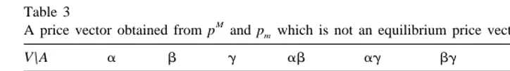
Note that choosing prices independently for each objecta between p (a) and p (ma) does not generally lead to a vector of equilibrium prices, as shown by the following example.
Example 3.11. Let e[´be such that I5h1,2,3j,V5ha,b,gj. The reservation values of the agents for the different subsets of objects are given in Table 3.
For this economy the efficient assignment is s(1)5habj, s(2)5[, s(3)5hgj. The
M
vectors p and pm are
M
p 5(7,8,7), pm5(4,7,6)
The price vector p5(4,7,7) however is not an equilibrium price vector since at these prices agent 3 would demand objectaand not objectg. The prices of objects need to be compatible: in particular the surplus of agent 3 on objectghas to be as least as large as on object a. The set of equilibrium prices is h(41e,7, p(g))u6#p(g)#min(61e,7)), 0#´#3j.
4. Relation between the cardinality condition and gross substitutability
We mentioned in Section 1 and in Section 2 that, for submodular reservation values, the cardinality condition implies that agents’ demands satisfy the gross substitute property. We now formally prove this claim. The proof uses the following properties of agents’ demands when their reservation value functions satisfy submodularity and the cardinality condition.
Lemma 4.1. Suppose that the reservation value V(i,?) of agent i is submodular and
1. if A and B are two subsets of D(i,p), and if uBu,uAu, then for everyasuch thata[A,
a[⁄ B, then B<ais in D(i,p)
2. if p and p9 are two vectors of prices such that p9$p, if A is a subset of D(i,p) of
maximum cardinality, then for all B[D(i,p9), uBu#uAu.
Proof.
1. uBu,uAu implies uB<au#uAu so that V(i,B<a)2V(i,B )$V(i,A)2V(i,A•a)$p(a), where the last inequality comes from the fact that A[D(i, p). Thus the surplus of
agent i with the objects of B<a is at least as large as with the objects of B, so that
B<a[D(i, p).
2. Suppose uBu.uAu. Then there exists b such that b[B, b[⁄ A. Since uA<bu#uBu,
V(i,A<b)2V(i,A)$V(i,B•b)2V(i,B )$p9(b)$p(b). Thus A<bis in D(i, p), which contradicts the assumption that A has the maximum number of elements among the subsets of D(i, p). h
Proposition 4.2. Suppose that the reservation value V(i,?) of agent i is submodular and
satisfies the cardinality condition. Then agent i’s demand satisfies the gross substitute
property.
Proof. Let p9be a price vector such that p9$p and let abe an element of D(i, p) such that p(a)5p9(a). By Lemma 4.1 demand (1), there is a subset uAu of maximum cardinality among the subsets of D(i, p) such thata[A. Let B[D(i, p9). By Lemma 4.1 demand (2),uBu#uAu. Ifa[⁄ B anduBu,uAu, then V(i,B<a)2V(i,B )$V(i,A)2V(i,A•a)$
p(a)5p9(a), so that B<a[D(i, p9). Ifa[⁄ B anduAu5uBu, there exists b[B, b[⁄ A. By Lemma 3.2, V(i,B•b<a)2V(i,B )5V(i,A)2V(i,A•a<b)$p(a)2p(b)$p9(a)2p9(b) where the last two inequalities come from the facts that A is at least as desirable at prices p than A•a<b, that p(a)5p9(a), and p9(b)$p(b). Thus B•b<a[D(i, p9) so that a[D(i, p9).h
Table 4
Free parameters with the cardinality condition
V \A a b g ab ag bg abg
V(1,A) 10 8 2 17 11 9 $17,#19
V(2,A) 8 5 10 11 16 13 $16,#21
V(3,A) 1 1 8 2 9 9 $9,#10
the cardinality condition satisfied, we can keep the same reservation values for objects a,b,g and the reservation values for one of the subsets composed of two objects (for example we keep the numbers in the column bg). Then the choice of numbers in this column determines all other reservation values for groups of two objects (since the marginal contribution ofa andgto one-object subsets are determined). The values for the three-object subset abg are then ‘free’ parameters (subject to the submodularity condition and monotonicity, that we have not used in the proofs, but is a natural assumption to require). For example, if we keep the same values for V(i,b<g) as in the original example, then the reservation values table must be as shown in Table 4.
If we only require that the demands satisfy the gross substitute property, then the only restrictions on the agents’ reservation values for subsets of two objects are as follows: if
V(i,a1<a2)2V(i,a2),V(i,a1<a3)2V(i,a3) then it must be that V(i,a1<a3)2V(i,a1)5
V(i,a2<a3)2V(i,a2). For if, for example, we had V(i,a1<a3)2V(i,a1).V(i,a2<a3)2
V(i,a2) then for prices p such that V(i,a1<a2)2V(i,a2),p(a1),V(i,a1<a3)2V(i,a3),
V(i,a2<a3)2V(i,a2),p(a3),V(i,a1<a3)2V(i,a1) and V(i,a2)2p(a2)5V(i,a1<a3)2
p(a1)2p(a3), agent i’s demand would consist of the setsha1,a3jandha2j. If the price
3
p(a1) slightly increases then the demand reduces to ha2j, which violates the gross substitute property. A similar reasoning eliminates the possibility that V(i,a1<a3)2
V(i,a1),V(i,a2<a3)2V(i,a2). Thus, when the column V(i,b<g) is chosen, there are still some degrees of freedom for choosing the values of V(i,a<b) and V(i,a<g) compatible with the GS property of the demand. For example, we could keep the two columns ag and bg of the original table, and the table of numbers has just to be modified so as to satisfy (Table 5).
Thus there are more ‘free’ parameters with the GS assumption than with the cardinality condition. It would be interesting to characterize all reservation value functions which lead to demands satisfying the GS property, in order to find which
Table 5
Free parameters with the gross substitute condition
V \A a b g ab ag bg abg
V(1,A) 10 8 2 10#V(1,a<b)#17 11 9 $maxh11,V(1,a<b)j
#11V(1,a<b)
V(2,A) 8 5 10 11 14 13 $14,#17
V(3,A) 1 1 8 1#V(3,a<b)#2 9 9 $9,#81V(3,a<b)
3
interpretable restrictions on the preferences of the agents are compatible with the GS property. Hopefully, future research will provide an answer to this question.
Acknowledgements
This paper was developed while the first author was visiting the Economics Department at the University of California, Davis, and the third author was visiting the Economics Department at Brown University. The hospitality of both departments is gratefully acknowledged. We thank H. Moulin and D. Perez for helpful comments. The first and third authors are also grateful for the financial support of the Spanish Ministry
´
of Education, Instituto Valenciano de Investigaciones Economicas, and D.G.I.C.Y.T under project PB93-6940.
Appendix A
Proof of Lemma 3.3
Step 1: Lettbe an efficient assignment ofV•a among I. Partition the set I of agents between the subsets
I15
h
i[Iuut(i )u.us(i )uj
, I25h
i[Iuut(i )u5us(i )uj
, I35h
i[Iuut(i )u,us(i )uj
and suppose that I is not empty, that is for some i1 [I,ut(i )u.us(i )u. Choose an agent
i[I . There exist b[t(i ) such that b[s( j ) for some agent j±i. 1
Suppose first that j[I , i.e.3 ut( j )u,us( j )u. Consider a new assignmentt* where agent j gets t( j )<b and agent i gets t(i )•b. Since ut( j )u,us( j )u, ut( j )<bu#us( j )u, then by Assumption SC we obtain that
V( j,t( j )<b)2V( j,t( j ))$V( j,s( j ))2V( j,s( j )•b)
Since s is an efficient assignment of V among I,
V( j,s( j ))2V( j,s( j )•b)$V(i,s(i )<b)2V(i,s(i ))
Since us(i )u,ut(i )u,us(i )<bu#ut(i )u, and by Assumption SC,
V(i,s(i )<b)2V(i,s(i ))$V(i,t(i ))2V(i,t(i )•b)
Therefore,
V( j,t( j )<b)2V( j,t( j ))$V(i,t(i ))2V(i,t(i )•b)
among I. Thus there must be equality, and the new assignmentt* obtained by shiftingb from agent i to agent j is an efficient assignment ofV•aamong I which has decreased by one the number of objects attributed to the agents of I .1
Suppose now that ut( j )u$us( j )u, that is j[I1<I . Then there exists an object2 b1 in t( j ) which is not in s( j ) and is thus in s( j ) for some agent j . For symmetry of1 1
notation call j the agent who has0 b unders( j5j ) and call0 b5b0. If j is in I then1 3
consider the assignmentt* obtained by transferringb0to agent j and0 b1to agent j . If1
agent j is in I1 1<I , then continue the procedure by finding an object2 b2 int( j ) which1
is not ins( j ) and is thus in1 s( j ) for some agent j . . . until an agent of I is reached.2 2 3
If the same agent in I1<I is selected at several stages of the procedure always choose a2
new object, so that b ±b ±b ±. . . . This is possible since for these agents ut(i )u$
0 1 2
us(i )u so that each object which is attributed to i under s and not under t has been replaced by a new object. Since I is non-empty, (there are less objects in3 V•athan in V) after a finite number of steps the procedure must stop by reaching an agent j in I .k 3
Consider the assignment t* obtained by transferring b0 from i to j ,0 b1 from j0 to
j , . . . ,1 bk to j . Note that without loss of generality we can assume that the agentsk
j , j , . . . , j are all different. For if the same agent is chosen at different stages of the0 1 k
procedure, i.e. if, for ,$0, r$1, j,5j,1 , then it is possible to choose directly the
r
objectb,1r11instead ofb,11int( j ) the first time that agent j is reached, avoiding the, ,
cycle j , j, ,11, . . . , j,1r. Let us show that the assignment t* is efficient. Applying Lemma 3.2 with C5t( j ), •b,11 and D5s( j ), •b, gives for agents j , . . . , j0 k21
V( j ,,t( j ), •b,11<b,)2V( j ,,t( j )), 5V( j ,,s( j )), 2V( j ,,s( j ), •b,<b,11) For agent i, since ut(i )u.us(i )u, by the cardinality condition
V(i,s(i )<b0)2V(i,s(i ))$V(i,t(i ))2V(i,t(i )•b0) and for agent j , sincek ut( j )uk ,us( j )uk
V( j ,kt( j )k <bk)2V( j ,kt( j ))k $V( j ,ks( j ))k 2V( j ,ks( j )k •bk)
Adding up these equalities and inequalities leads to
[V(i,t(i )•b0)1V( j ,0t( j )0 •b1<b0)1 ? ? ? 1V( j ,kt( j )k <bk)] 2[V(i,t(i ))1V( j ,0t( j ))0 1 ? ? ? 1V( j ,kt( j ))]k
$[V(i,s(i ))1V( j ,0s( j ))0 1 ? ? ? 1V( j ,ks( j ))]k
2[V(i,s(i )<b0)1V( j ,0s( j )0 •b0<b1)1 ? ? ? 1V( j ,ks( j )k •bk)] $0
where the last inequality is implied by the efficiency ofs.
Thus as long as an efficient assignment tof V•a is such that I is not empty it is1
possible to construct another efficient assignment t* with one less object attributed to the agents of I and one more to the agents of I . In a finite number of such steps we1 3
˜
Step 2: Consider now an efficient assignment rof V<a and partition the set I into
J15
h
i[Iuus(i )u.ur(i )uj
, J25h
i[Iuus(i )u5ur(i )uj
, J35h
i[Iuus(i )u,ur(i )uj
from agent j0 to agent i and note that the new assignment r9 obtained in this way
˜
belongs toS9(I,V<a). If agent j is in J stop here. If agent j is in J0 3 0 1<J there is an2
˜
objectb1which is ins( j ) and not in0 r( j ) (with the same convention for0 aanda) and is therefore in r( j ) for some agent j different from j . Transfer1 1 0 b1 from j to j and1 0
continue the procedure until an agent of J is reached. This has to happen since the3
objectsb0,b1, . . . can be chosen to be different and some objects must belong to agents of J . The same type of equalities / inequalities as in Step 1 show that the new3
˜
assignment ofV<a so obtained is efficient and gives one more object to the agents of
J . Transferring objects to these agents must lead in a finite number of steps to an1
˜
efficient allocation of V<a for which the set J is empty.1
˜
Step 3: Letrbe an efficient assignment ofV<a, which, by Step 2, can be chosen such
¯ ¯
Adding these equalities and exploiting the optimality of sleads to
¯ ¯ ¯
V(i,r(i )•b<a)1V(i ,1 r(i )1 <b•a)$V(i,r(i ))1V(i ,1r(i ))1
so that the new assignment is as efficient as r.
If a[⁄ r(i ) continue following the objects which are assigned in the assignment1 r differently than ins: there existsb1inr(i ) which is not in1 s(i ) and thus which is in1 by a different object. Since there are a finite number of different objects, at some point
˜
an agent i must be reached such thatm a(ora) is inr(i ). Then replacem bbyafor agent
¯i, b1 by b for agent i , . . . ,1 a by bm21 for agent i . As explained in Step 1 them
¯
type of equalities than in the simple case where m51 considered above, combined with the optimality of s, implies that the assignment so obtained is as efficient as r.h
References
Bikhchandani, S., Mamer, J., 1997. Competitive equilibrium in an exchange economy with indivisibilities. Journal of Economic Theory 74, 385–413.
Gale, D., 1984. Equilibrium in a discrete exchange economy with money. International Journal of Game Theory 13, 61–64.
Gul, F., Stacchetti, E., 1996. Walrasian Equilibrium Without Complementarity. Mimeo. ´
Henry, C., 1970. Indivisibilite dans une Economie d’Echanges. Econometrica 38 (3), 542–558.
Kaneko, M., 1982. The central assignment game and the assignment markets. Journal of Mathematical Economics 10, 205–232.
Kaneko, M., Yamamoto, Y., 1986. The existence and computation of competitive equilibria in markets with an indivisible commodity. Journal of Economic Theory 38, 118–136.
Kelso, A.S., Crawford, V.P., 1982. Job matching, coalition formation, and gross substitutes. Econometrica 50 (6), 1483–1504.
Laan, G., Talman, D., Yang, Z., 1997. Existence of an equilibrium in a competitive economy of indivisibilities with money. Journal of Mathematical Economy 28 (1), 101–109.
Quinzii, M., 1984. Core and competitive equilibria with indivisibilities. International Journal of Game Theory 13, 41–60.
Roth, A.E., Oliveira Sotomayor, M.A., 1990. Two-Sided Matching. Cambridge University Press, Cambridge. Shapley, L.S., Shubik, M., 1972. The assignment game I: The core. International Journal of Game Theory 1,