Doing Rawls Justice: Evidence from the PSID
Antonio Abatemarco
Abstract
Distributive value judgments based on the ‘origins’ of economic inequalities (e.g. circumstances and responsible choices) are increasingly evoked to argue that ‘the worst form of inequality is to try to make unequal things equal’. However, one may reasonably agree that distributive value judgments should also account for the ‘consequences’ of economic inequalities in such a way as to (i) improve economic efficiency and (ii) prevent from subordination, exploitation and humiliation. In this way of thinking, by evoking the well-known Rawlsian ‘Fair Equality of Opportunity’ and ‘Difference Principle’, the author proposes a pragmatical non-parametric estimation strategy to compare income distributions in terms of Rawlsian inequity and its contribution to overall inequality. The latter methodology is applied to PSID data from 1999 to 2013 and compared with existing empirical evidences on Roemer’s (A Pragmatic Theory of Responsibility for the Egalitarian Planner, 1993, and Equality of Opportunity, 1998) inequality of opportunity. Remarkably, Rawlsian inequity is found between 56% and 65% of the overall income inequality, with an increasing pattern originating from the recent economic crisis.
JEL D63 I32 D3
Keywords Rawlsian justice; equality of opportunity; income distribution
Authors
Antonio Abatemarco, Department of Economics and Statistics, University of Salerno, Fisciano, Italy, [email protected]
Citation Antonio Abatemarco (2016). Doing Rawls Justice: Evidence from the PSID. Economics: The Open-Access, Open-Assessment E-Journal, 10 (2016-33): 1—39.
1 Introduction
“Conservative egalitarians have a dream. They dream of a society in which at some age all individuals have equal opportunities, and in which all inequalities in out-comes can be traced to responsible choices ... there is nothing in this picture which precludes the coexistence of misery and outrageous wealth ... All egalitarians do not have to share this dream, and one can rightly view it as a nightmare. [T]he bulk of the egalitarian program is precisely to fight against this view of social life, and to look for institutions that would enable the population to form a community in which values of solidarity and mutual care would be embodied in institutions and would guarantee that every individual ... would be preserved from subordination, exploitation, humilation” (Fleurbaey 2001, p. 526).
From the perspective of a conservative egalitarian, inequalities areillegitimate (and so, compensation deserving) orlegitimate(and so, not compensation deserv-ing) depending on their determinants (e.g., luck, responsible choices), or let’s say, origins. This view can be seen as innervating Sen’s (1992)capabilityapproach, as well as Roemer’s (1993, 1998) ideal ofleveling the playing field, orluck egali-tarianism(e.g., Dworkin 1981a, 1981b, Cohen 1989), andstrict egalitarianism of opportunity(Arneson 1999).
Differently, outcome egalitarians deny that members of a society are ever non-identical in a distributively important sense. Here, it is said, in the name of individual responsibility and meritocracy, human rights of equal respect, equal social status and participation in democratic arenas are often violated in such a way as to welcome oppression and destitution (Anderson 1999). In this view, inequalities are said to be illegitimate due to their immediateconsequences– e.g., subordination, exploitation and humilation – whatever theirorigins. To the extent that one or the other perspective – origins, or consequences – is spoused, any attempt to reconcile distributive judgments is deemed to fail.
The contribution of this paper intends to be both methodological and empirical. From a methodological point of view, we propose a ‘pragmatical’ approach by which inequity – Rawlsian in spirit – can be (non-parametrically) estimated from income distributions. In this scenario, any pairwise disparity is said to be legitimate if it is (i) “attached to offices and positions open to all under conditions of fair equality of opportunity”, and (ii) “to the greatest benefit of the least-advantaged members of society” (Rawls 2001). As such, Rawls’ meritocracy is defined in a broader setting where both (i)fairnessof inequality origins, and (ii)goodnessof inequality consequences for the society as a whole, are simultaneously accounted for.
From an empirical point of view, given the separation betweensocialand natu-ralcircumstances that is innervating Rawls’ thought (Sugden 1993), US income distributions from 1999 to 2013 are compared over time in terms of both Rawlsian inequity and its contribution to overall inequality. Given the PSID resources (Panel Study of Income Dynamics), 64 subgroups are generated from the combination of two binarysocialcircumstances (i.e., place of origin and economic situation of parents in the early years) and four binarynaturalcircumstances (i.e., gender, health status in the early years, ethnicity, IQ-score). Iniquitous income disparities are found to account for 55.7–64.9% of overall outcome inequality. As compared to the 15–20% of iniquitous income disparities as estimated for Roemer’s inequality of opportunity (Pistolesi 2009, Abatemarco 2015), our analysis highlights that opting for the Rawlsian idea of justice more than doubles the share of illegitimate inequalities in the US.
our proposal for the non-parametric estimation of Rawlsian inequity is applied to US income distributions from 1999 to 2013. Section 5 concludes.
2 Rawlsian Equity
Following the old tradition of ‘social contract theory’ – whose best known pro-ponents are Hobbes, Locke and Rousseau – Rawls (1971) proposed a normative framework inspired by the ideal ofsocial cooperationfor the constitution of a well-ordered societywhere thestability of political institutionsis achieved through the legitimation of social and economic inequalities (reciprocity principle).
Rawls’ proposal is grounded on two basic value judgments which are known as theLibertyand theEqualityprinciple. According to the former, “Each person is to have an equal right to the most extensive total system of equal basic liberties compatible with a similar system of liberty for all”. This is indicated by Rawls as the principle having priority over the second one which is the one we focus on in what follows.
TheEqualityprinciple consists of two ethical value judgments for the identifi-cation of fair/good social and economic inequalities within an equity perspective: Fair Equality of Opportunity(hereafter, FEO) andDifference Principle(hereafter, DP). By FEO, social and economic inequalities “are to be attached to offices and positions open to all under conditions of fair equality of opportunity”, whereas, by DP, these inequalities are additionally required “to be to the greatest benefit of the least-advantaged members of society” (Rawls 2001).
of Sen’sleximinprinciple to preserve consistency with strong Pareto efficiency). Furthermore, for the same reason the Rawlsian theory of justice goes well beyond the basic foundations of egalitarianism of opportunity.
In what follows, we recall the basic foundations of both FEO and DP sepa-rately, the main objective being the identification of criteria by which a separating line is drawn between legitimate and illegitimate (pairwise) outcome inequalities according to our interpretation of Rawls’ theory.1
2.1 Fair Equality of Opportunity
According to Westen (1985), equality of opportunity is a three-way relationship between a person, some obstacles and a desired goal. A person only has an oppor-tunity if she has a chance of achieving that goal, meanwhile opportunities are equal if each individual faces the same relevant obstacles, none insurmountable, with respect to achieving the same desirable goal. In this view, inequality of opportunity concerns the distribution of obstacles only.
Similarly, FEO requires that citizens have the same educational and economic opportunities (obstacles) regardless of whether they were born rich or poor: “In all parts of society there are to be roughly the same prospects of culture and achieve-ment for those similarly motivated and endowed” (Rawls 2001). As such, FEO emphasizes the role of institutions, which are required to grant to all individuals equal command over resources. Basically, in Rawls’ view the society is intended as asystem of fair cooperationwhere “what has to be distributed justly – or fairly – are the benefits and burdens of social cooperation” (Sugden 1993). In this sense, optimal redistributive policies concern the distribution of social (e.g. training and education costs), not natural (e.g. talent) resources.2
Notably, Rawls’ view has been criticized by Sen (1992) as “equal command over resources can coexist with unequal real opportunities because individuals
1 Strictly speaking, Rawls proposal is a theory of ‘background procedural justice’ where all outcome
inequalities are said to be legitimate whenever resulting from a well-ordered society.
2 The interpretation of Rawls’fair equality of opportunityas proposed in this paper is not the only
differ in their ability to convert resources into functionings”. Evidently, Sen and Rawls’ views originate from two very different definitions of opportunity. In Rawls’ view, an opportunity is intended as a ‘chance of access to resources’, whereas Sen refers to an opportunity as a ‘chance of outcome’ (or outcome prospect).3
This aspect of Rawlsian justice is particularly relevant when considering FEO as one of the two criteria that outcome inequalities are required to satisfy to be regarded as legitimate. Since inequalities must “be attached to offices and posi-tions open to all under condiposi-tions of fair equality of opportunity” (Rawls 2001), if outcome inequalities occur between individuals with the same endowment of socialresources (e.g., economic conditions of parents in the early years, access to public services in the place of origin), then this inequality is said to be fair.
Here, we propose an extension of this idea by claiming that outcome inequal-ities arefair if and only if unequal access to social resources cannot be said to be one of the ‘determinants’ of inequality. In this sense, social and economic inequalities are required to be ‘complaint-free’ in the view of the Rawlsian ideal of social cooperation and stability, independently of the contribution of un/fairness to the single outcome gap. This is of moral importance in itself as, in this view, which clearly differs from Roemer’s ideal ofleveling the playing field, any pairwise outcome gap is said to be unfair even if it is partly but not entirely originating from unequal social circumstances.4
According to this extension of Rawls’ FEO, we claim that if the outcome dis-parity benefits the least endowed individual (e.g., with no access to same offices and positions as the other individual), it must be the case that fairness holds once again.5 This consideration is not superfluous because outcomes, as remarked by Sen’s critique above, are not uniquely generated by social resources, i.e., better out-comes might be achieved by individuals with worse endowment of social resources because of different natural resources, or even luck (e.g., Lefranc et al. 2009).
3 In a sense, this debate resembles the old distinction betweenformalandsubstantiveequality of
opportunity (Rosenfeld 1986).
4 As such, a distinction is made between fair and unfair disparities, independently of the monetization
of the contribution of circumstances and responsible choices which is implicitly assumed for the parametric estimation of equality of opportunity (e.g., Bourguignon et al. 2007).
5 A similar procedure has been already implemented in the empirical strategy proposed by
So said, we claim that, in Rawls’ view, pairwise outcome disparities areunfair, and so,illegitimate, if and only if the better-off individual coincides with the better endowed one in terms of social resources. On the other hand, pairwise outcome disparities arefair, and not yetlegitimate(as goodness is also required), whenever the better-off individual is not the better endowed one in terms of social resources.
2.2 Difference Principle
In Rawls’ view,fairnessof social and economic inequalities is ruled by FEO, mean-whilegoodnesscomes from DP. Specifically, DP poses an additional condition to be verified to make social and economic inequalities legitimate, by which social institutions be arranged so that financial inequalities are to everyone’s advantage, and specifically, to the greatest advantage of those advantaged least (Wenar 2012). Remarkably, to the extent that income inequalities are said to be good if generating benefits for the whole population, and especially for the worst-off, Rawlsian meritocracy takes into account theconsequencesof inequalities, besides their origins (i.e., responsibilities or circumstances).6 As such, the theory of justice as fairness goes definitely beyond the idea of equalizing opportunities. Also, as merit is defined by considering social consequences of inequalities, not just individual ones, DP is meant to be a threat tomethodological individualism characterizing most of the standard economic theory.
Drawing from DP, two major implications can be emphasized. First, DP recalls one of the most relevant debates in the economic theory, that is the identification of the ‘effects of inequality on growth’. Second, since growth is required to benefit especially the worst-off, poverty is crucial. In this sense, the Rawlsian theory of justice relies, among all, on the capacity of social and economic inequalities to generate growth, which is additionally required to be of the ‘pro-poor’ kind.
It turns out that DP concerns theindirecteffect of inequality on poverty through growth, which is not to be confused with the direct effect (e.g., Bourguignon 2005) by which any inequality reducing transfer is inevitably poverty reducing (independently of growth) when the donor is non-poor whereas the recipient is
6 ”[Rawls] argues that after establishing equality of opportunity, rational individuals would tolerate
poor, and vice versa. Differently, in the Rawlsian view, inequalities are good whenever they are (i) growth enhancing, and (ii) to the greater benefit to the poorest individuals.
As such, the definition of a methodology for the empirical estimation of Rawlsian equity passes inevitably through the identification of implementable criteria by which good and bad (pairwise) inequalities can be identified according to their impact on (i) growth determinants, and (ii) pro-poor growth, which is not straightforward at all. In what follows, we consider both aspects separately.
a) Inequality on growth
In this section, we argue that any pairwise outcome inequality can be said to be growth enhancing if (i) the disparity is not jeopardizing individual opportunities to access profitable investments in terms of both human and physical capital accumulation, and (ii) the disparity enforces effort and economic incentives in general. In what follows, we offer a justification for this claim. More specifically, given the most relevant growth determinants as identified in Barro’s (1998) seminal paper,7consequences of pairwise inequalities in terms of growth are delineated by evaluating the impact of such inequalities on each growth determinant.
According to Barro, “[long-run or steady-state level of per capita output] depends on an array of choice and environmental variables. The private sector’s choices include saving rates, labor supply, and fertility rates, each of which depends on preferences and costs. The government’s choices involve spending in various categories, tax rates, the extent of distortions of markets and business decisions, maintenance of the rule of law and property rights, and the degree of political freedom”.
Let’s consider first the effect of inequality on the saving rate. On one hand, inequality affects the saving rate by giving to few people a better and deeper chance to invest in resource-demanding activities which would not be undertaken otherwise. This applies to both physical (e.g., Kaldor 1957) and human capital (e.g., Barro 2000, Wenar 2012). On the other hand, in the presence of credit market
7 Undoubtedly, the identification of growth determinants is an open debate, and several additional
imperfections, inequality, by enlarging the set of people who may have access to profitable investments in human and physical capital, may increase efficiency, and so generate growth (Galor and Zeira 1993). These two causalities evidently conflict with each other. However, the latter is known to dominate the former on the basis of empirical evidences.8
Let’s now turn to the second determinant of growth as indicated by Barro. Labor supply is clearly affected by inequality as well. Compressed wage structures that do not reward merit will lead to more equal societies, but it is also likely that they will reduce workers’ incentives to put in additional effort or aim at outstanding achievements (Mirrlees 1971). “Good inequalities are those that reflect and reinforce market-based incentives that are needed to foster innovation, entrepreneurship and growth” (Chaudhuri and Ravallion 2006). In this sense, the principle of reward,9 by which inequalities determined by responsible choices (e.g., effort) are legitimate (and not to be compensated), is implicitly relevant in Rawlsian justice as “institutions promote or restrict growth according to the protection they accord to effort” (Lewis 2013). Nevertheless, in contrast with Roemer’sleveling of the playing field, here, rewarding effort is to be intended as a step toward meritocracy, not meritocracy itself.
Then, from the former two growth determinants (i.e., saving rate and labor supply), we can infer that pairwise inequalities are expected to affect growth through (i) individual opportunities to access profitable investments in terms of both physical and human capital accumulation, and (ii) the optimal design of
eco-8 In a sequence that mirrors intellectual fashions on the empirics of growth, researchers have looked
at rates of growth over long periods of time (e.g., Persson and Tabellini 1996, Perotti 1996, Alesina and Rodrik 1994), the level of income across countries (Easterly 2007), and the duration of growth spells (Berg, Ostry and Zettelmeyer 2012), and have found that inequality is associated with slower and less durable growth. The few exceptions (Forbes 2000, Banerjee and Duflo 2003) tend to pick up ambiguous short-run correlations (Aghion, Caroli, and Garcia-Penalosa 1999, Halter, Oechslin, and Zweimï¿œller 2014). According to Galor and Moav (2004), the dominating causality strongly depends on the degree of development in the society; more precisely, the positive effect of inequality is expect to prevail in developing countries only.
nomic incentives. In addition, for the rest of the growth determinants mentioned above, the way inequality may affect growth basically replicates these two ratio-nales.10
b) Growth on poverty
The impact of growth on poverty rates has been the object of vibrant debates among those who believe that growth is itself the best anti-poverty policy and those who argue that growth is not necessarily alleviating poverty within a market economy.
According to the first view, Dollar and Kraay (2002) show empirically that the income of the poor rises one-for-one with overall growth.11 As such, Dollar and Kraay conclude that governments need not follow pro-poor growth policies; they should simply maximize economic growth provided they avoid high inflation and maintain fiscal discipline.
In contrast, some others have observed that economic growth in the last decades has not changed the degree of relative inequality, meaning that, the proportional benefits of growth going to the poor are the same as those enjoyed by the non-poor. According to this view, Kakwani and Pernia (2000) observe that “the growth process that results from market forces generally benefits the rich proportionally
10Fertility is a standard variable in basic growth models. An impact of inequality on the endogenous
fertility rate may exist if poor families show higher fertility rates and lower investment capacity (Schultz 1989, and Barro and Lee 1994). Then, in the presence of credit market imperfections, since access to profitable investments in human capital is not granted to the increasing part of the population, inequality lowers growth (de la Croix and Doepke 2003). Similarly, market distortions due to government choices alter individual opportunities to invest in human or physical capital and/or economic incentives. In this sense, Alesina and Rodrik (1994) observe that high inequality enlarges the demand for (distorting) redistribution of the median-voter due to the lognormal distribution of income. Finally, as observed by Barro (1998), democracy is relevant for growth because, “in extreme dictatorships, an increase in political rights tends to raise growth because the limitation on governmental authority is critical. However, in places that have already achieved some political rights, further democratization may retard growth because of the heightened concern with social programs and income redistribution”. Then, dictatorship limits individual liberties and so the possibility to exploit profitable investment, meanwhile excessive democratization may jeopardize, once again, economic incentives (Bourguignon and Verdier 2000).
11This general relationship between the income of the poor and per capita GDP growth holds in a
more than the poor. This is because the rich have inherent advantages (e.g., human and material capital) in a market economy”.
It is evident in itself that the basic foundation of pro-poor growth is strictly related to Rawls’ (1971)maximinprinciple. Even more, in line with Kakwani and Pernia (2000), DP clearly progresses in the direction of pro-poor growth by claiming that growth is desirable to the extent that it is to the greatest benefit of the neediest part of the population.
Given Rawls’ focus on pro-poor growth, it is worth observing that, within this literature, several definitions of pro-poor growth have been proposed. For some observers, growth is pro-poor if it leads to any reduction in poverty (e.g., Ravallion and Chen 2003, Ravallion 2004); for others, it is pro-poor only if it leads to a disproportionate increase in the incomes of the poor, that is, if it is associated with declining inequality (e.g., White and Anderson 2000).12
The former definition of pro-poor growth is much less strict and focuses solely on the link between poverty and growth; a growth episode is said to be pro-poor if poverty falls regardless of the developments on the inequality front. The second definition, instead, would basically require that the income share of the poor population increases. The simplest version of this definition is based on a relative concept of inequality and would simply state that the growth rate of the income of the poorest individuals is greater than the average growth rate (White and Anderson 2000).13
To the extent that growth is to benefitmorethe least well off, Rawls’ DP clearly evokes the latter approach, that is, growth is of the pro-poor kind if it reduces both poverty and inequality. In this sense, DP resembles the definition of the Asian Development Bank (ADB 1999) by which “growth is pro-poor when ... accompanied by policies and programs that mitigate inequalities and facilitate income and employment generation for the poor, particularly women and other
12Specifically, the major benefit for the poorest part of the population can be defined in absolute or
relative terms, depending on the use of money measures or shares (e.g., Bibi et al. 2012).
13Another version of this definition is proposed by Kakwani and Pernia (2000) where poverty
traditionally excluded groups”.14
The latter definition, in line with Rawls’ idea ofequal command over resources, emphasizes the role of opportunities of access to income and employment positions. In this sense, “[pro-poor growth is obtained by removingartificial barriers to entry into certain trades and professions, or into the formal labor market in general ... [through] adequate public spending for basic education, health and family planning services, improved access to credit, and the promotion of small and medium enterprises” (Kakwani and Pernia 2000).
As such, we argue that in order to generate pro-poor growth, pairwise outcome inequalities must not be jeopardizing the opportunities of access to profitable investments in human and physical capital accumulation. As this statement is the same as the first condition obtained in the previous section (i.e., for pairwise inequalities to be growth enhancing), in our view, growth-enhancing pairwise inequalities are generally expected to generate growth of the pro-poor kind (not vice versa). Notably, this does not mean that growth is generally pro-poor (i.e., pro-poor growth policies are useless), but that growth originating from pairwise inequalities is always pro-poor.
Summing up, according to our interpretation of Rawlsian justice, pairwise outcome inequalities aregoodby DP (not necessarilylegitimate), if (i) disparities enforce effort and economic incentives, and (ii) disparities do not jeopardize individual opportunities to access profitable investments in terms of both human and physical capital accumulation. In addition, to belegitimate, pairwise outcome disparities are required (iii) to befair by FEO, that is, the better-off individual must not be the better endowed one in terms ofcommand over (social) resources.
14This is additionally supported by empirical evidences showing that pro-poor growth originates
3 A Non-Parametric Pragmatic Estimation Strategy
3.1 Formal Definitions
Given a population of N individuals, let {y1, ...,yN} ∈ℜN+ be the increasingly
ordered outcome vector whereyis the socioeconomic variable which, without loss of generality, may be intended as income.
Each individual is associated with a set ofznnaturalcircumstances{n1, ...,nzn} identifying genetic traits (e.g., gender, cognitive abilities). Moreover, each individ-ual is characterized by a finite set ofsocialcircumstances{s1, ...,szs}indicating the social environment in the early years (e.g., parental income, access to public services/facilities). Evidently, both natural and social circumstances are intended as beyond individual control.
For each natural circumstance, letnq:={n1q, ...,n τq
q}be the vector indicating
τqmutually exclusive discrete values (e.g., male or female) associated to theqth
natural circumstance variable (e.g., gender). Similarly, letsq:={s1q, ...,s τq
q }be the
vector indicatingτq mutually exclusive discrete values (e.g., high/medium/low)
associated to theqth social circumstance variable (e.g., parental income). We define theithnatural opportunity type(θn
i) as a combination of discrete
values (e.g., male and Hispanic) associated with each natural circumstance variable (e.g., gender and cognitive abilities), i.e. θn
i = (nα1 ∩...∩nωzn). Similarly, theith social opportunity type(θs
i) is defined as a combination of discrete values (e.g., low
parental income and high public services performances) associated with each social circumstance variable (e.g., gender and cognitive abilities), i.e.θs
i = (sα1∩...∩sωzs). Given the finite set of natural opportunity typesΘn:={{θn
i }ni¯=1}and social opportunity typesΘs:={{θs
i}si¯=1}, let define withΘ:={{θin}in¯=1,{θsj}s¯j=1}the finite set ofopportunity profiles, each one indicating a single natural and social opportunity type respectively, which can be reformulated asΘ:={θk}kn¯=×s1¯. E.g., if natural circumstances consist of gender (male or female) and cognitive abil-ities (high or low), whereas social circumstances are parental income (low or high) and public services performances in the place of origin (low or high), then
¯
n= (2)2 and ¯s= (2)2. In addition, the set of opportunity profiles consists of
(n¯×s¯) = (2)2×(2)2= (2)4different opportunity types.
respect to theirresponsibility type(e.g., effort). More specifically, letE :={ei}e¯ i=1 be the finite set of responsibility types. We assume thaty= f(θn,θs,e) is the
income generating function where f:Θn×Θs×E →ℜ
+. Evidently, income is
expected to increase when natural or social opportunity type improves, as well as when the responsibility type is better. As such, the definition of an empirical strat-egy crucially depends on the identification of both opportunity and responsibility orderings, that is not straightforward as strong assumptions are inevitably required. In what follows, we opt for anordinalpragmatic approach.15
Opportunity Orderings
Given the vector indicatingτq mutually exclusive discrete values (e.g., high or
low cognitive abilities, male or female) associated to theqth natural circumstance variable (e.g., cognitive abilities, gender), i.e.nq:={n1q, ...,n
τq
q}, we assume that
discrete values can be completely ordered in terms ofpropitiousnesswithin the income generating process (e.g., high cognitive abilities more propitious than low ones) independent of other circumstances and responsible choices. Formally, this means that, holding fixed the rest of the natural and social circumstance variables and the responsibility type, for each pair of values{nαq,nβq}(originating the two
natural opportunity typesθn
i andθnj respectively), and according to existing social
conditions (which may differ over time and across geographical areas), one may reasonably expect eitheryθn
i,θ¯s,e¯= f(θ
Given a complete ordering among discrete values associated to each natural
15For cardinal approaches quantifying the contribution of effort and circumstance within the income
generating function see, Bourguignon et al. (2007), Checchi et al. (2008), Pistolesi (2009), Ferreira and Gignoux (2011), and Almas et al. (2011).
16Even if the possibility of orderings of opportunity sets has been already considered in the existing
circumstance, let {θn
1, ...,θn¯n} be the set of natural opportunity profiles and let
yi jk indicate the income unit with theith natural opportunity type, thejth social
opportunity type and the kth responsibility type. We define the partial natural opportunity ordering≻n
θ as follows: (i)yi jk≻nθ ym jk, wheneverθincan be obtained
from θn
m by selecting more propitious values for some natural circumstance
variable(s) without worsening any other, and (ii)yi jk||nθym jk(non-comparability),
whenever θn
i can be obtained fromθmn by selecting more propitious values for
some natural circumstance variable(s) but less propitious for some other(s). We write n
θ and∼nθ to indicate the asymmetric and symmetric component of the
natural opportunity ordering respectively.
For instance, let cognitive abilities (high, low) and gender (male, female) be the only two (binary) natural circumstance variables. Since being ‘high’ and ‘male’ is usually found to be more propitious in the income generating process, then, by virtue of the natural opportunity ordering above, ‘low’-‘males’ benefit of a better natural opportunity type with respect to ‘low’-‘females’, but the former is not comparable with the natural opportunity type consisting of ‘high’-‘females’.
Evidently, the same formal framework can be replicated for social circumstance variables. Once again, we assume that discrete values (e.g., high or low)) asso-ciated to theqth social circumstance variable (e.g., parental income in the early years) can be completely ordered in terms ofpropitiousnesswithin the income generating process, independently of other circumstances and responsible choices. Formally, holding fixed the rest of the natural and social circumstance variables and the responsibility type, for each pair of values{sαq,sβq}- originating the two
social opportunity typesθs
i and θsj respectively - it is reasonable to expect, on
a priorigrounds, eitheryθ¯n,θs
1, ...,θss¯}be the set of natural opportunity profiles. Thepartial social
opportunity ordering≻s
θ is defined as follows: (i)yi jk≻sθ yiok, wheneverθiscan be
obtained fromθs
oby selecting more propitious values for some social circumstance
variable(s) without worsening any other, and (ii)yi jk||sθyiok(non-comparability),
wheneverθs
i can be obtained fromθosby selecting more propitious values for some
circumstance variable(s) but less propitious some other(s). We writes
θ and∼sθ
ordering respectively.
Finally, let’s recall the finite set of opportunity profiles Θ :=
{{θn
i}ni¯=1,{θsj}s¯j=1}. We define the opportunity profiles ordering ≻θ as
fol-lows: (i)yi jk≻θ ymok, wheneveryi jkθn ymokandyi jksθ ymokwith at least one of
the two preferences holding strictly, (ii)yi jk||θymok(non-comparability), whenever
yi jk≻nθ ymokandyi jk≺sθ ymok, oryi jk≺θn ymok andyi jk≻sθ ymok, oryi jk||nθymok, or
yi jk||sθymok. Once again, we write θ and ∼θ to indicate the asymmetric and
symmetric component of the opportunity profiles ordering respectively.
Responsibility Ordering
In line with Roemer’s (1993) pragmatic theory, if a disjoint and exhaustive partition rule is assumed to exist by which individuals within the same population can be grouped depending on the opportunity profile (accounting for both natural and social circumstances), two individuals belonging to different subgroups are said to becomparablein terms of responsible choices (not necessarily the same degree of responsibility) if they are equally ranked in the respective subgroup income distributions. In this sense, the income gap among equally ranked individuals may capture the contribution of circumstances to overall inequality.
Here, a more demanding pragmatic approach is proposed by which rank-based partial responsibility orderingsare defined (Abatemarco 2010). Given the disjoint and exhaustive partition of the population with respect to the finite set of opportunity profilesΘ:={θk}nk¯×=1s¯, letFk(y)be the subgroup cumulative frequency distribution
associated to thekth opportunity profile. Letφ(·)be a monotone transformation and yikthe income of theith individual associated to thekth opportunity profile, we
iden-tify the responsibility type ofyikwith the intervalφ[Fk(yi−1,k)]<eik≤φ[Fk(yik)].
As such, the partial responsibility ordering≻ecan be (pragmatically) defined as
follows: (i) ifFk(yi−1,k)≥Fh(yjh)thenyik≻eyjh, (b) ifFk(yik)≤Fh(yj−1,h)then
yjh≻eyik, (c) ifFk(yi−1,k) =Fh(yj−1,h)andFk(yik) =Fh(yjh)thenyik∼eyjh, and
(d) the income units are non-responsibility comparable otherwise (yik||eyjh).17 The
asymmetric component of the responsibility ordering is indicated bye.
17For instance, given two increasingly ordered subgroup income vectors,x:={x
1,x2}andy:= {y1,y2,y3}, thenx2≻ex1,y3≻ey2≻ey1,y3≻ex1andx2≻ey1, while the couples(x1,y1),(x1,y2),
Within the rank-based approach, since individuals belonging to the same sub-group are characterized by the same opportunity type, within-sub-group income gaps are unequivocally ascribed to different responsible choices. As such, rank-based responsibility orderings allow to overcome very information demanding processes which would inevitably be required otherwise. However, this is not afree-meal. To the extent that some circumstances may be unobservable at reasonable costs, individuals within the same subgroup may indeed differ from each other in terms of circumstances, and the rank-based ordering would erroneously legitimate such income disparities in the name of nonexisting differences in terms of responsible choices. This is a relevant problem which is known to afflict both parametric and non-parametric estimation strategies (Ramos and Van de gaer 2012). In this context, we argue thatpartialresponsibility orderings are definitely to be preferred with respect tocompleteones, as this may allow the mitigation of distortions originating from unobserved circumstances.
An additional consideration concerns theindirecteffect of circumstances; it is known that responsible choices may be significantly influenced by circumstances (e.g., Bourguignon et al. 2007). In this sense, it is worth observing that the rank-based approach automatically accounts for the indirect effect because responsibility orderings are invariant with respect to both translations and scale transformations applied to each subgroup.
3.2 Fairness and Goodness
According to FEO, pairwise income inequalities are fair whenever the better-off individual did not enjoy any advantage in terms of access to social resources; as we said above, in line with the Rawlsian ideal of social cooperation, we assume that fairness holds if the disparity is complaint-free in terms of command over social resources, whatever the size of the contribution of unfairness to the income gap. As such, fairness of pairwise income inequalities can be defined as follows.
Definition 3.1 (Fairness) Given the finite set of social opportunity typesΘs:=
{θs
i}si¯=1and the income distribution{y1, ...,yN} ∈ℜN+ withyj>yi,
3.1.i)ifyjsθ yi, then|yj−yi|is fair;
3.1.ii)ifyj≻sθ yioryj||sθyi, then|yj−yi|is not fair.
To the extent that the sole social circumstance variables are accounted for, Rawl-sian fairness in Definition 3.1 differs with respect to the standardcompensation principlefor two reasons at least. First, Rawlsian fairness is not sufficient to claim legitimacy of an income gap, and so compensation deservingness. Second, natural circumstances are not accounted at all, as fairness is uniquely concerned with institutions intended as a system of fair cooperation.
Rawlsian fairness is a necessary but not sufficient condition forlegitimacyof pairwise inequalities, as the additional criterion to be considered for sufficiency purposes is goodness. In turn, as argued above, by virtue of DP, two necessary conditions are required for goodness, i.e. (i) income disparities must enforce effort and economic incentives (hereafter, incentive-based goodness), and (ii) income disparities must not jeopardize individual opportunities to access profitable in-vestments in terms of both human and physical capital accumulation (hereafter, access-based goodness). Remarkably, the simultaneous verification of both condi-tions is sufficient and necessary for an income disparity to be good.
Definition 3.2 (Incentive-based Goodness) Given the finite set of opportunity profilesΘ:={θi}in¯=×1s¯and the income distribution{y1, ...,yN} ∈ℜN+ withyj>yi,
3.2.i)ifyj≻eyi, then|yj−yi|is good for incentives;
3.2.ii)ifyjeyi, oryj||eyi, then|yj−yi|is not good for incentives.
As such, Definition 3.2 resembles the principle of reward as intended by Ar-neson’s (1999)strict egalitarianism of opportunity, where maximum equality of opportunity is obtained if “no one is worse off than others through no fault or voluntary choice of her own”. Notice that, to be coherent with Rawlsian framework, reward has not to be regarded as thelegitimateprize for better individual respon-sible choices. Here, reward isborneto the extent that it represents an incentive to better responsible choices, which are expected to be growth enhancing in the interest of the society as a whole. Most importantly, alegitimateprize does not need to beincentivizing, and vice versa.
responsible choices and circumstances we have opted for, because a distinction is made between good and non-good income disparities without any possibility to separate the good from the non-good component in every single income gap. Differently, to the extent that the contribution of circumstances and responsible choices within the income function is monetized (i.e., parametric approach), good inequalities may be identified according to the principle of naturalreward, by which the effect of heterogeneous circumstances are to be canceled out across the entire population, or, alternatively, according to the principle ofutilitarianreward, by which heterogeneous circumstances are to be canceled out across equally de-serving individuals in such a way as to maximize the sum of individual utilities.
Moving a step forward, as observed above, in order to be good, pairwise income inequalities are additionally required to be not jeopardizing individual opportuni-ties to access profitable investments in terms of both human and physical capital accumulation. The very basic question to be answered is the following: when do pairwise income inequalities jeopardize individual opportunities of access? Evidently, an answer to this question cannot be given independently of a definition of access opportunities.
From a methodological point of view, opportunities of access can be differently defined depending on the main objectives. For instance, within a strictly dichotomic approach, one may say that two individuals differ in terms of opportunities of ac-cess when acac-cess is granted to one but not to the other. However, if the dichotomic approach is abandoned, opportunities of access may still differ in magnitude even if access is granted to both individuals.
In this paper, as we aim at separating pairwise inequalities which jeopardize access opportunities from the rest of pairwise inequalities, we opt for the former approach, that is, we claim that access is not granted for socially excluded individu-als, and vice versa (i.e., it is the status of poor that really matters, not the size of the poverty gap). As such,access-based goodnesscan be formally defined as follows.
Definition 3.3 (Access-based Goodness) Given the income distribution {y1, ...,yN} ∈ ℜ+N with yj >yi, let z be the poverty line capturing social
ex-clusion in the society,
3.3.i)ifyi>z, oryj≤z, then|yj−yi|is not bad for access;
Basically, by Definition 3.3, any pairwise income inequality jeopardizes access opportunities for one of the two individuals whenever the income disparity is associated with an access disparity as well. On the contrary, if the income disparity does not concur with an access disparity, then such inequality is not said to be jeop-ardizing access. Intuitively, goodness cannot hold whenever the income disparity can be said to be contributing to the generation of access disparities. Remarkably, by claiming that a necessary (but not sufficient) condition to legitimize social and economic inequalities is that such a disparity should be notresponsiblefor poorness, our interpretation of DP principle is coherent with Rawlsian maximin principle.18
3.3 Gini-based Aggregation
Recalling formal definitions in the previous Section, Ralwsian equity can be reformulated as follows.
Definition 3.4 (Rawlsian Equality Principle) Given the income distribution {y1, ...,yN} ∈ℜ+N withyj>yi and the poverty linezcapturing social exclusion in
a specific society, letΘs:={θs
i}si¯=1 be the finite set of social opportunity types, andΘ:={θi}in¯=×1s¯the finite set of opportunity profiles,
I)if|yj−yi|satisfies (3.1.i), (3.2.i), and (3.3.i), then|yj−yi|is legitimate;
II)if (3.1.i), or (3.2.i), or (3.3.i)does not hold, then|yj−yi|is illegitimate.
As compared to egalitarianism of opportunity, social and economic inequalities are said to be legitimate to the extent that rewarding effort at the individual level, that is assumed to be growth enhancing, is not poverty enhancing, given that fair equality of opportunity has been granted.19
According to Definition 3.4, inequity is given by the aggregation of income gaps satisfying condition(II), meaning that equity differs from equality due to legitimate income inequalities(I). Specifically, for measurement purposes, in line
18To the extent that the income thresholdzis country-specific, Definition 3.3 allows to account
for the heterogeneity of institutional contexts which clearly matters for the identification of social exclusion.
19“Thus the principles of social justice are macro and not necessarily micro principles” (Rawls
with the old tradition of the Gini index, we opted for the unweighted aggregation of income gaps, even if weighted aggregation functions may be supported as well. LetΩbe the set of pairwise income gaps satisfying conditions(I)in Definition 3.4, given income distribution{y1, ...,yN} ∈ℜN+, inequality is measured as,
where µ stands for mean income. Most importantly, following the same logic behind Dagum’s (1997) decomposition (two-components),Gcan be decomposed as follows
where the second component in squared brackets captures inequity. As such, we measure Rawlsian inequity (GR) as
GR=
where the contribution of Rawlsian inequity to overall inequality is defined as
GcR= GR
G (4)
The inequity indexGR(andGcR) is scale invariant, partially symmetric in
Cow-ell’s (1980) sense, and defined in[0,1]. In addition, it is replication invariant to the extent that a k-fold replication of the entire population refers to all the characteris-tics of each income unit (i.e., income, responsibility type, social opportunity type).
Any non-reranking rich-to-poor transfer (hereafter, PD transfer) betweenykand
yhis inequity reducing wheneverh,k6∈ω. Also, it can be shown that, givenyk>yh
withk∈Ωandh6∈Ω, any PD transfer is inequity reducing wheneveryh<y˜with
˜
yindicating the median income for alli6∈Ω. Similarly, givenyk>yhwithk6∈Ω
the median income for alli6∈Ω.
According to this framework, it must be the case that inequity is null when inequality is null, but not vice versa. Mostly, perfect equity may be attained in the presence of social and economic inequalities. Proposition 3.1 makes the point.
Proposition 3.1 (Perfect Equity) Given the set of natural and social opportunity typesΘn:={θn
i }ni¯=1andΘs:={θis}is¯=1respectively, letΘ:={θi}ni¯=×1s¯be the set of opportunity profiles whose corresponding subgroup income distributions are
¯
yi :={y1i,y2i, ...}, and let {y1, ...,yN} ∈ℜN+ be the income distribution where
∃i:yi6=yj. The two following statements are equivalent.
i)GR=0.
ii)(a.)∀i,j,θn
i 6=θnj ⇔θi6=θj;
(b.)∃i: ¯yj is a k-fold replication of ¯yi∀ j, and
(c.)yi≥z∀i, oryi<z∀i.
Proof 3.1 Givenθi6=θjif and only ifθin6=θnj, it must beyi∼sθ yj∀i,jby which
(3.1.i) holds for all|yj−yi|. Similarly, ifyi≥z∀i, oryi<z∀i, then (3.3.i) holds
for all |yj−yi|. Finally, if each subgroup, as obtained through a disjoint and
exhaustive partition w.r.t. {θi}ni¯=×1s¯, is the k-fold replication of another subgroup, thenyi=yj∀i,j:yi∼eyj andyj>yi∀i,j:yj ≻eyi. As such, (3.2.i) holds for
all|yj−yi|. This proves thatGR=0. On the other hand, given{y1, ...,yN} ∈ℜN+
such that∃i:yi6=yj (i.e.,G6=0), ifGR=0, we prove that all pairwise income
inequalities must be Rawlsian equitable according to Definition 3.4. GivenGR=
0, by (3.2.ii), if yj ∼e yi, or yj||eyi, then it must be yj =yi∀i,j. As such, by
definition of≺e, if{y1, ...,yN} ∈ℜN+is such that∃i:yi6=yj, then each subgroup
associated to an opportunity profile must be the k-fold replication of another subgroup. Indicating byNithe size of the ith subgroup, this ensures thatNj=kjNi
for all subgroups, withkj being any positive integer. By (3.3.ii), |yj−yi|=0
wheneveryj ≥z>yi, which is possible if and only if allyi≥z∀i, oryi<z∀i.
Finally, given that (i) {y1, ...,yN} ∈ℜN+ is such that ∃i:yi 6=yj, (ii) i,j∈θk
implies i,j∈θs
h∀i,j,k,h, and (iii) each subgroup is the k-fold replication of
another subgroup, let’s assume, by contradiction, that∃i,j:yj ≻θs yi, oryj||sθyi
(i.e., (3.1.ii)), by which two subgroups differ from each other with respect toθs. It
at least one unfair inequality, which would contradictGR=0. As such, it must be
the case thatyi∼sθ yj∀i,j.
Proposition 3.1 emphasizes that within the Rawlsian view, the focus is on a social system of fair cooperation where the same opportunities of investments in human and physical capital must be granted to everybody. In addition, in line with a broader interpretation of the maximin principle, equity is maximized when there is no group of more disadvantaged individuals, or, equivalently, all of them are disadvantaged. Finally, given these two conditions above, inequalities can be tolerated if and only if these are determined by effort in such a way as to be growth but not poverty enhancing. In this sense, as compared to Roemer’s ideal of leveling the playing field, the applicability of the principle of reward is restricted a prioriby additional normative requirements concerning theconsequencesof income disparities.
4 An Empirical Application to PSID
4.1 Data
The PSID20 is used to compare US income distributions over time in terms of Rawlsian equity as defined above. This database has been preferred due to (i) the availability of information on most of the natural and social circumstance variables, and (ii) the high number of records. The former aspect is crucial because, as we observed above, omitted variables may cause the misleading legitimation of illegitimate income gaps, which may seriously jeopardize the reliability of major empirical findings (Ramos and van de Gaer 2012). The latter aspect is crucial as well; to the extent that the initial population is to be partitioned into several subgroups, a high number of observations is required to ensure a sufficient number of records in each subgroup (Ferreira and Gignoux 2011).
To facilitate the comparison with the existing empirical literature, we consider the same initial wave as in Abatemarco (2015), where the evolution of equality
20Panel Study of Income Dynamics public use dataset. Produced and distributed by the Institute for
of opportunity in the US is measured according to Roemer’s idea ofleveling the playing field. More specifically, eight waves are considered from 1999 to 2013 (1999, 2001, 2003, 2005, 2007, 2009, 2011, 2013).21
We refer to the sole population of heads aged less than 80 years old. Evidently, the estimation of the impact of circumstance and effort variables on the income generating function requires a population of individuals, not households. In addi-tion, we choose to focus on the sole population of heads because (i) the decisions of non-heads are usually more influenced by family needs than heads’ ones, and (ii) some variables are not available for non-heads (e.g., taxable income).
Income is measured in disposable terms. More specifically, disposable income is defined as total income from labor and capital investments plus public (monetary) transfers minus income and property taxes.22 Poverty thresholds for each wave are taken from publicly available data of the US Census Bureau.23
According to the distinction between natural and social circumstances, we consider fournaturalcircumstance variables, i.e. gender, health status in the early years (before 16–17 years old), ethnicity, and IQ score24, and twosocial circum-stance variables, i.e. economic situation of parents in the early years, and place of origin in the early years.25
Remarkably, we consider health status in the early years and not current health, as (i) the latter is more informative about chances given to each individual to invest
21Income data refer to the previous chronological year (e.g., 1999 income records refer to 1998). 22Total income is determined by head’s income from labor, asset, trust fund, dividends, and interest.
To account for the Federal Income Tax, brackets and tax rates from 1998 to 2012 have been considered. The property tax is entirely imputed to the head when single, whereas it is halved for married heads. To save as many observations as possible, missing values for each income variable (e.g. 1999) have been been replaced by the corresponding value of the same respondent as resulting from the subsequent wave (e.g. 2001) if available. Finally, outliers in the distribution of disposable income have been dropped by eliminating observations below and above the 5th and the 95th centile respectively (e.g. Jarvis and Jenkins 1998).
23Data for unrelated individuals available at https://www.census.gov/hhes/www/poverty/data/threshld/. 24The introduction of a proxy for cognitive abilities (IQ test) within the set of circumstance variables
is not straightforward from a philosophical point of view because a trade-off may occur between different social and ethical objectives, that is, the“above notion of equality of opportunity may contradict other ethical principles such as self-ownership and freedom” (Lefranc et al. 2008).
25To preserve a sufficient number of observations, missing values are replaced by records available
in human capital accumulation, and (ii) it is less influenced by responsible choices even if, as observed by Sen (2002), the impact of responsible choices may be ambiguous in this field “since we tend to give priority to good health when we have the real opportunity to choose”. In addition, as compared to Abatemarco (2015), for our purposes the place of origin is not considered in terms of employment opportunities (i.e. unemployment rate in the place of origin in the early years), but as the characterization of opportunities given to an individual to invest in human capital accumulation whenever willing to. This aspect is captured by using information on the degree of urbanization in the place where the respondent grew up (i.e., farm, rural area, small town, large city).
Binary circumstance variables are defined even if, except for gender, more than two alternatives are available from the PSID. This choice is to be intended as a compromise aimed at minimizing the loss of information. On the one hand, an increase in the number of alternatives for each variable would grant more precise information at the individual level. On the other hand, the number of subgroups would exponentially increase with a serious loss of information due to the lack of statistical significance for many subgroups.
As such, 64 subgroups are generated from the combination of six binary cir-cumstances: gender (male [M], female [F]), health in the early years (no health problems [H], health problems [ ¯H]), ethnicity (propitious [E], non-propitious [ ¯E]), IQ score (high [I], low [ ¯I]), economic situation of parents in the early years (pretty well off [W], non-pretty well off [ ¯W]), and place of origin (low [U], high [ ¯U]).26
26To construct each subgroup, both the PSID family and the PSID individual data files have been
Subgroups with less than five observations have been disregarded.
The number of observations varies across waves from a minimum of 4,999 to a maximum of 6,146 records, which is enough to grant statistical significance of the results.27 In addition, from 1999 to 2013, the population consists of 66–69% male, 76–81% had no health problems, 21–27% pretty well-off parents, 50–66% are of a propitious ethnicity, 55–57% showed high IQ scores and 37–40% were from highly urbanized areas.
The average disposable income is 27.422 USD in 1999, 29,796 USD in 2001, 29,794 USD in 2003, 31,542 USD in 2005, 34,474 USD in 2007, 35,148 USD in 2009, 32,741 USD in 2011, and 33,962 USD in 2013. Given the focus on the population of heads, these statistics confirm previous evidences in the existing literature (Heathcote et al. 2009).
Income data are disaggregated at the subgroup level in Table 1, where subgroups are grouped on the basis of the number of favorable circumstances from the better-off to the worst-better-off. Reasonably, subgroup average income is increasing with the number of favorable circumstances. More specifically, to highlight the contribution of each circumstance variable, correlation matrices have been computed between circumstance variables and disposable income (Table A.1, Appendix). By the latter,
(e.g., French, German) or “religious” (e.g., Jewish, Catholic) and the others reporting “hyphenated American”, “non-specific Hispanic identify”, “racial” or “other”. This partition is supported by empirical evidence on average disposable incomes for each group (Abatemarco 2015). IQ test records are obtained from the family data file for the 1968 and the 1972 waves. The latter variables have been associated with the corresponding income units from the 1999 to the 2013 waves using family, not person identifier, i.e., the IQ score is not referred to the single individual but the family. The IQ score is assumed to be low whenever (i) family has been interviewed in both waves, obtaining a score that is below the median score in both waves, or (ii) family has been interviewed in one of the two waves and is positioned below the median score. For the economic situation of parents in the early years, the population has been partitioned by drawing a separating line between individuals reporting “pretty well off” and the remaining population answering “poor” or “average”. This definition is primarily aimed at the identification of true benefits in the income generating process due to family origins. Finally, the place of origin is assumed to limit access to profitable investment in human capital if individuals grew up in a “farm”, or “rural area”, “suburb”, or “small town” as compared to opportunities offered by “large cities”.
27Subgroups with less than five observations are considered statistically insignificant and are
Tab. 1: Groups of subgroups average disposable incomes (thousand dollars) and shares by number of favorable circumstances
1999 2001 2003 2005
ID No.F. (%) $1000 (%) $1000 (%) $1000 (%) $1000 1 6 0.02 43.0 0.02 38.5 0.03 44.3 0.02 43.9 2-7 5 0.16 36.1 0.17 39.5 0.16 37.4 0.15 41.0 8-22 4 0.29 29.4 0.30 32.8 0.31 32.1 0.30 34.1 23-42 3 0.29 26.6 0.28 26.9 0.28 28.1 0.30 29.3 43-57 2 0.17 20.2 0.16 22.9 0.15 22.6 0.17 25.6 58-63 1 0.05 15.9 0.05 17.5 0.05 14.9 0.05 17.9 64 0 0.01 13.1 0.01 10.3 0.01 11.2 0.00 16.8
2007 2009 2011 2013
ID No.F. (%) $1000 (%) $1000 (%) $1000 (%) $1000 1 6 0.01 48.6 0.02 44.3 0.02 38.9 0.02 37.4 2-7 5 0.13 42.8 0.14 42.2 0.13 38.9 0.14 40.3 8-22 4 0.32 39.2 0.33 39.1 0.32 35.8 0.33 37.2 23-42 3 0.31 32.2 0.31 33.0 0.31 31.4 0.30 31.9 43-57 2 0.16 27.4 0.15 28.2 0.16 27.0 0.16 28.9 58-63 1 0.06 19.8 0.04 20.4 0.05 21.6 0.05 22.4 64 0 0.01 17.5 0.00 23.7 0.00 18.8 0.00 21.8
Each group of subgroups (ID:={1, ...,64}) is characterized by the same number of favorable circumstances (No.F.). Average disposable incomes (thousand US dollars) and frequencies (%) are reported for each group and wave. Source: author’s computation on PSID data.
it turns out thatnaturalcircumstance variables are much more relevant thansocial ones within the income generating process. Remarkably, the degree of urbanization in the place of origin and economic conditions of parents in the early years seem to have a non-significant impact on disposable income.
4.2 Results
In this section, we discuss the results of the empirical methodology we have proposed for the estimation of Rawlsian inequity. As such, we do not discuss immediate policy implications as this would go beyond the scopes of this paper. On the contrary, the reliability of our results is verified by considering previous evidences on inequality of outcomes and opportunities in the US.
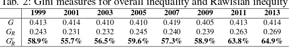
Tab. 2: Gini measures for overall inequality and Rawlsian inequity
1999 2001 2003 2005 2007 2009 2011 2013 G 0.413 0.414 0.410 0.410 0.419 0.405 0.413 0.414
GR 0.243 0.231 0.232 0.245 0.240 0.239 0.263 0.269
Gc
R 58.9% 55.7% 56.5% 59.6% 57.3% 58.9% 63.8% 64.9%
Gini’s decomposition. Source: author’s computation on PSID data.
heads aged, on average, between 42 and 44 years old, the Gini index is found between 0.405 and 0.419 from 1999 to 2013 (Table 2). This result is consistent with previous findings in Heathcote et al. (2009), where inequality is found to be sensibly larger in the population of singles28(income pooling within married households reduces inequality) and is increasing with the age of the sample (early retirements and the experience wage premium usually increase inequality).
As reported in Table 2, Rawlsian inequity from 1999 to 2013 is found to be between 55.7% and 64.9% of the overall inequality. This result sensibly differs with respect to previous parametric and non-parametric empirical evidences for Roemer’s inequality of opportunity, which is usually found between 15% and 20% (Abatemarco 2015, Pistolesi 2009). Nevertheless, this is just what one may expect; Roemer’s view is grounded on the legitimation of income gaps with respect to the sole origins of inequality, whereas Rawlsian inequity is defined by accounting for both the origins and the implications of income inequality.
Additional information can be obtained by considering the dynamics of inequity from 1999 to 2013. Starting from 2007, a rapid increase in the absolute and relative amount of inequity can be observed. This is evidently determined by the financial crisis in 2007, whose major effects are detected since 2009. The main rationale behind the impact of this crisis on Rawlsian inequity appears immediately from Table 3, where the contribution of FEO and DP are computed separately.29
Both FEO and DP have sensibly increased in the latter three waves. However,
28Evidently, the population of singles is not the same as the population of heads, but the latter
definitely accentuates the share of singles.
29We report the contribution of FEO and DP, as considered separately, and not the decomposition
Tab. 3: Rawlsian inequity decomposition by FEO and DP
1999 2001 2003 2005 2007 2009 2011 2013 Gc
R (58.9%) (55.7%) (56.5%) (59.6%) (57.3%) (58.9%) (63.8%) (64.9%)
Gc
R(FEO) 28.1% 25.5% 27.3% 31.8% 30.8% 31.7% 35.9% 37.4%
Gc
R(DP) 43.8% 41.7% 42.1% 42.3% 41.7% 43.3% 47.4% 49.6%
Gc
R(DP1) 9.3% 8.6% 8.2% 8 .4% 9.1% 9.1% 10.7% 13.1%
Gc
R(DP2) 39.5% 37.7% 38.5% 38.9% 38.5% 40.7% 44.5% 46.9%
Gc
R(FEO) andGcR(DP) indicate the shares of illegitimate income disparities whenever FEO and DP are
separately accounted for respectively. Similarly,Gc
R(DP1) andGcR(DP2) account for illegitimate income
disparities due to failure of (3.2.i) and (3.3.i) respectively. Source: author’s computation on PSID data.
by considering separately the contribution of “incentive-based goodness” (DP1) and “access-based goodness” (DP2), it can be observed that the financial crisis has mostly worsened the existing poverty conditions, so that a larger share of income inequality is found to cause social exclusion and limited access to profitable investments in human and physical capital.
Remarkably, in addition to the (expected) impact of the financial crisis on poverty, and so Rawlsian inequity, Table 3 also highlights a relevant contribution of FEO, whose increase from 1999 is even stronger than that of DP. According to our framework, this means that the financial crisis has been paid relatively more by individuals with poor parental origins in rural areas.
Finally, the U-shaped pattern of DP1 in Table 2 suggests that the financial crisis has seriously jeopardized the capacity of the economic system to reward better responsible choices. A discussion on the motivations of this result, although of crucial importance for the design of optimal redistributive policies, is beyond the aims of this paper. For our purposes, it is enough observe that this result confirms previous evidences on the U-shaped pattern of Roemer’s inequality of opportunity (Abatemarco 2015).
5 Conclusive Remarks
no valid judgments are agreed upon by which some inequalities may be said to be fair/good, or some equalities are said to be unfair/bad, equality is said to be equitable or just.
In the recent times, most of the research effort in the empirical literature has been devoted to the estimation of inequality of opportunity, meanwhile Rawls’ ideal of asystem of fair cooperationaimed at social and politicalstabilityhas been mostly disregarded in this sense. The success of egalitarianism of opportunity is somehow related to the increasing concern for ‘individual responsibility’ characterizing the Protestant culture (Fleurbaey 2001). Nevertheless, to the extent that egalitarianism of opportunity characterizes Rawlsian theory as well, we suggest that such a minor interest for Rawlsian Principle of Equality can be better motivated by theoretical impediments in accommodating the Difference Principle within the standard economic theory.
In this paper, RawlsianFair Equality of OpportunityandDifference Principle have been interpreted in such a way as to render Rawlsian equitypragmatically workable within an empirical setting. Undeniably, Rawls’ theory of justice is less user-friendly and much more information demanding than other approaches, but, to our opinion, this should not be a valid reason for abandonment.
A methodology for non-parametric estimation of Rawlsian inequity has been proposed. The latter approach has been implemented to calculate the contribution of Rawlsian inequity to overall income inequality in the USA from 1999 to 2013. Iniquitous income disparities are found to account for 56–65% of overall outcome inequality, which more than doubles the usual 15–20% of iniquitous income disparities as estimated for Roemer’s inequality of opportunity (Abatemarco 2013, Pistolesi 2009). Even worse, our analysis suggests that, due to the recent financial and economic crisis, the huge amount of inequity is found to be rapidly increasing in the last waves.
because welfare improvements in terms of equality of opportunity may be offset by increasing subordination, exploitation, and humilation if implemented.
Appendix
Tab. A.1: Correlation matrices
1999 Income Gender Health Urbanization Parents Ethnicity IQ Score
Income 1
Gender 0.28 1
Health 0.14 0.09 1
Urbanization 0.01 -0.07 -0.01 1
Parents 0.06 -0.01 0.04 0.05 1
Ethnicity 0.17 0.13 0.06 -0.08 -0.01 1
IQ Score 0.18 0.10 0.07 0.00 0.05 0.25 1
2001 Income Gender Health Urbanization Parents Ethnicity IQ Score
Income 1
Gender 0.27 1
Health 0.15 0.08 1
Urbanization 0.00 -0.08 -0.01 1
Parents 0.10 0.03 0.02 0.05 1
Ethnicity 0.16 0.13 0.07 -0.10 -0.01 1
IQ Score 0.19 0.10 0.07 -0.00 0.04 0.26 1
2003 Income Gender Health Urbanization Parents Ethnicity IQ Score
Income 1
Gender 0.27 1
Health 0.11 0.06 1
Urbanization 0.01 -0.09 -0.02 1
Parents 0.08 0.01 0.04 0.03 1
Ethnicity 0.14 0.12 0.05 -0.10 -0.01 1