Full Terms & Conditions of access and use can be found at
http://www.tandfonline.com/action/journalInformation?journalCode=ubes20
Download by: [Universitas Maritim Raja Ali Haji] Date: 12 January 2016, At: 22:50
Journal of Business & Economic Statistics
ISSN: 0735-0015 (Print) 1537-2707 (Online) Journal homepage: http://www.tandfonline.com/loi/ubes20
Clustering of Auto Supplier Plants in the United
States
Thomas Klier & Daniel P McMillen
To cite this article: Thomas Klier & Daniel P McMillen (2008) Clustering of Auto Supplier Plants in the United States, Journal of Business & Economic Statistics, 26:4, 460-471, DOI: 10.1198/073500107000000188
To link to this article: http://dx.doi.org/10.1198/073500107000000188
Published online: 01 Jan 2012.
Submit your article to this journal
Article views: 301
Clustering of Auto Supplier Plants in the United
States: Generalized Method of Moments
Spatial Logit for Large Samples
Thomas KLIER
Federal Reserve Bank of Chicago, Research Department, Chicago, IL 60604 (tklier@frbchi.org)
Daniel P. MCMILLEN
Department of Economics (MC 144), University of Illinois at Chicago, Chicago, IL 60607 (mcmillen@uic.edu)
A linearized logit version of Pinkse and Slade’s spatial GMM estimator reduces estimation to two steps— standard logit followed by two-stage least squares. Linearization produces a model that can be estimated using large datasets. Monte Carlo experiments suggest that the linearized model accurately identifies the presence of spatial effects and is capable of producing accurate estimates of marginal effects. In an application to the location of supplier plants in the U.S. auto industry, the results imply no additional clustering of new plants beyond the level of clustering of existing plant locations.
KEY WORDS: Agglomeration; Automobile industry; Spatial GMM.
1. INTRODUCTION
Discrete-choice models can be problematic in spatial datasets because standard spatial models typically imply heteroscedas-ticity and autocorrelation. Full maximum likelihood estimation is problematic because the likelihood function involvesn inte-grals, wherenis the sample size. Several estimators have been proposed that are capable of producing consistent estimates when data are spatially autocorrelated and heteroscedastic— Case (1992), LeSage (2000), McMillen (1992), and Pinkse and Slade (1998). However, these estimators become infeasible for large samples because they require the inversion ofn×n ma-trices.
The primary objective of our article is to propose a compu-tationally feasible estimator for spatial discrete-choice models. Our estimator is a linearized version of the generalized method of moments (GMM) estimator proposed by Pinkse and Slade (1998). Linearization allows the model to be estimated in two steps. The first step is a standard probit or logit model, in which spatial autocorrelation and heteroscedasticity are ignored. The second step involves two-stage least squares estimates of the linearized model. The benefit of linearization is that no matrix needs to be inverted and estimation requires only standard pro-bit/logit models and linear two-stage least squares. Thus, the model can be estimated even with very large sample sizes.
Our estimator extends the literature on spatial modeling by allowing a model with a spatially weighted dependent vari-able to be estimated in a discrete-choice framework. For the case of continuous dependent variables, examples of this sort of model include Bordignon, Cerniglia, and Revelli (2003), Brett and Pinkse (2000), Brueckner (1998), Brueckner and Saavedra (2001), Case, Rosen, and Hines (1993), Fredriksson and Mil-limet (2002), Revelli (2003), and Saavedra (2000). The general model is writtenY=ρWY+Xβ+u, whereYis the dependent variable,W is the weight matrix,X is a matrix of explanatory variables,uis an error term, andρandβ are parameters whose values are to be estimated. Spatial effects are present if ρ is not equal to zero; values ofY are influenced by nearby values of Y, where “nearby” is defined implicitly by the prespecified
entries of the weight matrix. For example, Brueckner (1998) found that California municipalities are more apt to have re-strictive growth control measures if nearby municipalities are also highly restrictive. Current estimators for this class of spa-tial models are only suitable for models with continuous depen-dent variables. We extend these estimators to the case where the dependent variable of interest is discrete. Continuing with the example of growth controls, we reinterpretYas the underlying latent variable showing the strength of the tendency to adopt growth controls, which then is translated into a discrete vari-able showing whether the municipality has measures to control growth.
Monte Carlo experiments suggest that the linearized model accurately identifies spatial effects. Whenρ is small—from 0 to about .5—the linearized model shows no tendency toward excessive rejections of the null ofρ=0. As ρ increases, the linearized model eventually tends to overstate the value ofρ. However, the linearized model combined with one calculation of the full covariance matrix produces remarkably accurate es-timates of the marginal effects ofX.
In an empirical application to the location decisions of new auto supplier plants in the United States, the linearized logit model leads to the same qualitative results as full GMM es-timation. The auto industry is an interesting example because significant restructuring since the 1970s has altered the spatial distribution of supplier plants. Does the location of new plants simply follow the pattern already established in the areas that are attracting openings? Or do suppliers seek out locations that have not yet attracted other plants? The issue is important be-cause economic development agencies spend large sums to at-tract firms. Such policies may have little chance of success if they are designed to attract firms to remote locations when firms prefer to locate in areas close to other suppliers. Our results suggest that new plants tend to cluster together. However, once
© 2008 American Statistical Association Journal of Business & Economic Statistics October 2008, Vol. 26, No. 4 DOI 10.1198/073500107000000188
460
we control for proximity to existing plants, new plants show no
additionaltendency toward concentration. The shift of the in-dustry from an east–west to a north–south orientation has been accomplished by having new supplier plants mimic the location decisions of existing plants. The industry remains highly con-centrated, and Detroit continues to be its hub. Policies designed to attract firms to remote locations are unlikely to be successful.
2. SPATIAL DISCRETE–CHOICE MODELS
The spatial model is written in matrix notation as
Y=ρWY+Xβ+ε. (1)
The n×n matrix W is the “weight matrix.” In the typical specification,Wii=0 andnj=1Wij=1 for j=i. This speci-fication implies that each value of Y is a function of a group of explanatory variables,X, and a weighted average of the val-ues of the dependent variable for nearby observations. Coun-ties are the unit of observation in our application. We follow common practice and impose thatWij=1/ni for all counties that are contiguous to countyi, whereni is the number of ob-servations that are contiguous to countyi. Under this specifi-cation,W is sometimes referred to as the “contiguity matrix,” and the coefficientρ captures the spatial interaction effect. If
ρ >0, then high values ofY for nearby observations increase the value for observationi. In our formulation,ρ >0 implies clustering: the probability of having an auto supplier plant in a county increases if there are plants in neighboring counties. In contrast,ρ <0 implies dispersion as the probability decreases when there are plants in neighboring counties.
When the dependent variable is continuous, (1) is usually es-timated by maximum likelihood methods (Anselin 1988). Al-ternatively, Kelijian and Prucha (1998) proposed a GMM esti-mator for the model in which the spatial autoregressive term,
WY, is replaced by an instrumental variable, which is the pre-dicted value from a regression ofWYon a set of instruments,Z. The GMM estimator has two advantages over maximum likeli-hood estimation: (1) it does not rely on a potentially inaccurate assumption of normally distributed errors, and (2) by relying on two-stage least squares, estimation does not require calculating the determinants and inverses ofn×nmatrices. Although the primary advantage of maximum likelihood estimation is the po-tential for efficiency, one of the reasons why researchers con-sider employing a spatial model in the first place is the true structure of the model is rarely known. The specification ofW
is arbitrary, and researchers often try several different specifica-tions to figure out which one best captures the spatial patterns evident in the data. The prospect of efficiency becomes ques-tionable when the true model is uncertain. GMM estimation is more robust than maximum likelihood to departures from the restrictive assumptions required by the maximum likelihood es-timator.
When the dependent variable is discrete rather than contin-uous, maximum likelihood estimation is problematic because the likelihood function typically involvesn integrals. Several authors have proposed estimation procedures that maintain the structure implied by maximum likelihood estimation for the
spatial probit model. Case (1992) assumed a special, block di-agonal structure forW, which simplifies the estimation proce-dure substantially. For example, we might assume that all ob-servations within a state have a common spatial component:
Wij=1/(ns−1)for all observations (i=j) in states, where
ns is the number of observations in state s. However, this re-strictive specification does not allow the weights to decline with distance within a state. McMillen (1992) and LeSage (2000) based their estimators directly on (1) and (2). McMillen used an expectation-maximization (EM) algorithm to estimate the model under the assumption of normally distributed errors, whereas LeSage used a Bayesian approach based on Gibbs sampling to simulate the probabilities. Both approaches are limited to relatively small samples because they require the
n×nmatrix(I−ρW)−1to be inverted in each iteration. Beron and Vijverberg (2004) proposed an interesting but computation-intensive probit model using a GHK simulator to evaluate the
n-dimensional normal probability.
A variant of the Pinkse and Slade (1998) GMM estimator for a spatial discrete-choice model does not rely on the normality assumption. Their estimator is designed for a model with spa-tially dependent errors:
y=Xβ+e, e=θWe+ε=(I−θW)−1ε, (2) where ε is a vector of independent and identically distrib-uted errors. Equation (2) forms the basis for either a probit or a logit model; the discrete variable, d, equals 1 if y>0, andd=0 otherwise. The covariance matrix is proportional to
V(e)= [(I−θW)′(I−θW)]−1, and the variances are given by the diagonal elements, σi2. The model structure implies both heteroscedasticity and autocorrelation foreunlessθ=0.
Although Pinkse and Slade (1998) used (2) as the basis for a probit model, we will outline their estimator using the logit ap-proach that we employ in our empirical application. The prob-ability thatdi=1 is given byPi=exp(Xi∗β)/[1+exp(X∗iβ)], whereXi∗=Xi/σi, and the generalized logit residuals are sim-plyui=di−Pi. The GMM estimator is the set of values forβ andθ that minimizesu′ZMZ′u, whereZ is a matrix of instru-ments andM is a positive definite matrix. An interesting appli-cation of the Pinkse and Slade estimator for the probit case is found in Flores-Lagunes and Schnier (2005).
If M =(Z′Z)−1, the GMM estimator reduces to nonlinear two-stage least squares. The iterative procedure has the follow-ing steps:
The covariance matrix is given by
var(Ŵ)ˆ =(Gˆ′Gˆ)−1 dient term forρis much more complicated:
Gρi= −Pi(1−Pi)
Xi∗β σi2 ii,
where is the n×n matrix (I−ρW)−1W(I−ρW)−1(I−
ρW)−1. Note that reduces toW whenρ=0. SinceWii=0, the gradient term for ρ equals zero for all observations when
ρ=0.
This model extends readily to the model with a spatially lagged dependent variable. To do so, we must reinterpret (1) as the underlying latent variable explaining thepropensityto have
d=1. As the propensity to have d=1 increases for nearby observations, the propensity increases for observation i also. This assumption is different from a model in which the discrete variableddepends directly on neighboring values ofd, that is, whered=ρWd+Xβ+ε. It is also different from a model in which the value of the underlying variable depends on neigh-boring values ofd, so thaty=ρWd+Xβ+ε. These models are not algebraically consistent.
The assumption that the latent variable depends on spatially lagged values of the latent variable may be disputable in some settings. In our example, we are assuming that the propensity to locate a new supplier plant in a county depends on the propen-sity to locate plants in nearby counties, and it doesnotdepend simply on whether new plants have located nearby. The as-sumption is reasonable in this context because of the forward-looking nature of plant location decisions. Having other plants nearby may help lower costs by adding to the pool of labor with the skills desired by the industry. Similarly, having more plants in the area may attract specialized firms that produce in-puts to the auto supplier plants, and it may encourage state and local governments to invest in infrastructure valued by supplier plants. In Brueckner’s (2003) terminology, the auto supplier industry is characterized by a resource flow model, in which skilled labor, specialized suppliers, and local infrastructure are drawn to an area as auto supplier plants locate there. Thus, a firm’s costs are lower when it is not alone in an area. If firm location decisions are forward looking, then they may look for locations where other firms are expected to locate, that is, to places with high values of the latent variable. In this situation, firms expect that high values of the latent variable will attract other firms, which in turn will lower costs. In contrast, the spa-tial error model of (2) is more appropriate in a situation where plants are attracted to an area because of missing variables that are correlated over space. For example, an area may have an un-usually productive work force that attracts firms to an area. In practice, it often is difficult to distinguish between these models in a continuous dependent-variable setting. In the case of a dis-crete dependent variable, an additional attraction of the model with a spatially lagged latent dependent variable is that it leads to a particularly tractable estimation procedure based on a lin-earized version of the spatial autoregressive logit model.
Pinkse and Slade’s (1998) estimator is readily extended to a model with a spatially lagged dependent variable. Following the interpretation of (1) as the underlying latent variable for the discrete-choice model, we have
Y=(I−ρW)−1Xβ+(I−ρW)−1ε. (4) As in the Pinkse and Slade (1998) model, the covariance ma-trix is given by [(I−ρW)′(I−ρW)]−1 and the generalized derive a linearized version of the model.
3. THE LINEARIZED SPATIAL LOGIT MODEL
Although GMM estimation is robust to departures from the distributional assumption that is explicit in maximum likeli-hood estimation, the spatial probit and logit models remain computationally burdensome. Each step of the iterative esti-mation procedures requires the inversion of then×n matrix
(I−ρW). Yet the spatial model given by (1) is generally viewed as an approximation. We seldom know the true structure of the spatial dependence; what is known is that the errors tend to be correlated over space. Whereas the models implied by (1) and (2) were developed for the relatively small datasets that were common in the past, large datasets require less restrictive models that do not require inverting large matrices.
Because the model is already viewed as an approximation, a reasonable simplification is to make the approximation ex-plicit and linearize the model around a convenient starting point (see Greene 2002). In this case, the starting point is obvious: whenρ=0,βis estimated consistently by standard logit mod-els. And when ρ =0, no matrices need be inverted because
(I−ρW)−1=I. The gradient terms simplify substantially
be-With the linearized model, estimation involves the following steps:
(1) Estimate the model by standard logit. The estimated val-ues areβˆ0. Calculateu0 and the gradient terms,Gβi=
ˆ
Pi(1− ˆPi)XiandGρi= ˆPi(1− ˆPi)Hiβˆ, whereH=WX. (2) RegressGβ andGρ onZ. The predicted values are Gˆβ andGˆρ. Then regress u0+G′ββˆ0 on Gˆβ andGˆρ. The coefficients are the estimated values ofβandρ. No large matrices have to be inverted in this algorithm. All it requires is standard logit followed by two-step least squares.
The algorithm is closely related to the first step of the GMM estimator for the nonlinearized model, which is a regression of
u0onGˆβandGˆρ. Subsequent iterations of the full model would require calculating(I−ρW)−1, whereas the covariance matrix requires calculating(I−ρW)−1W(I−ρW)−1(I−ρW)−1. The spatial error model approach of Pinkse and Slade (1998) is not identified under the linearization approach because the gradi-ent for the spatial term is equal to zero whenρ=0. However, the first term in (6) allowsρto be estimated under the spatial model. If the true structure of the model is given by (1), lin-earization will provide accurate estimates as long asρis small, and in general, the linearized model will provide a good ap-proximation to the unknown underlying spatial model.
4. MONTE CARLO ANALYSIS
Previous studies (McMillen 1995; Beron and Vijverberg 2004) have used Monte Carlo procedures to establish that spa-tial effects produce severe bias in linear probability and stan-dard probit models. In this section we present the results of a set of Monte Carlo experiments that verify the usefulness of both the GMM and the linearized logit estimator for the spatial lag model. The basis for the experiments is a simple version of (1) with a single explanatory variable:Y=ρWY+β1+β2x+ε. The explanatory variable, x, is drawn from a U(−1,1) dis-tribution, and the same values of x are used for each repli-cation of an experiment. Letting X=(1,x),Xi∗=Xi/σi, and
To construct the dependent variable, we draw a vector of er-rorsefrom a U(0,1)distribution, and definedi=1 ifei≤Pi anddi=0 otherwise. This experimental setup assures that the assumptions behind the spatial logit model are met.
The main difficulty in setting up the Monte Carlo experi-ments is deciding on the structure of the weight matrix, W. GMM estimation involves invertingn×n matrices, and esti-mation quickly becomes intractable as sample sizes increase. Though the linearized logit model can easily be estimated for any sample size—indeed, that is one of its primary attractions— it is helpful to have the GMM estimator as a basis of compar-ison. Furthermore, constructing the base model requires calcu-lating(I−ρW)−1for linearized logit as well as for GMM esti-mation.
To make calculating(I−ρW)−1feasible in a Monte Carlo setting, we simplify the structure of the weight matrix in two ways. First, we take advantage of the approximation (I −
ρW)−1=I+ρW+ρ2W2+ρ3W3+ · · · to avoid having to calculate the inverse directly. In our Monte Carlo experiments, we use this third-order expansion to form the base model. The second simplifying assumption makes it possible to avoid work-ing with large matrices at all: we defineWi,j=.5 if|i−j| =1 (withW12=Wn,n−1=1). This form forWwould apply, for ex-ample, if the data were drawn from locations along a ray from a base point and the observations were ordered by distance. In this example, theW matrix is a standard first-order contiguity matrix, and it is easy to solve directly for(I−ρW)−1. These simplifications make Monte Carlo analysis feasible for large data sets while maintaining the essential structure of standard spatial models.
The number of observations varies between 1,000 and 10,000 and ρ varies from −.9 to .9, whereas β1 =0 and β2=1 throughout. We report standard logit estimates of β1 and β2, along with linearized logit and GMM estimates of β1, β2, andρ. To save space, we present a subset of the full results; the full set of results is available on request. The instruments for both GMM and linearized logit estimation are a constant,x,
Wx,W2x, andW3x. Note that because the scale of the logistic distribution is 1, the variance isσ2=π2/3. All three estima-tors provide estimates ofβ/σ rather thanβ (the spatial coeffi-cientρis not affected by the scaling). Thus, we reportβˆ0
√
3/π
andβˆ1
√
3/π rather thanβˆ0andβˆ1. We run 1,000 replications
of each experiment, and summarize the results by the mean, standard deviation, and root mean squared error (RMSE) of the 1,000 sets of estimates.
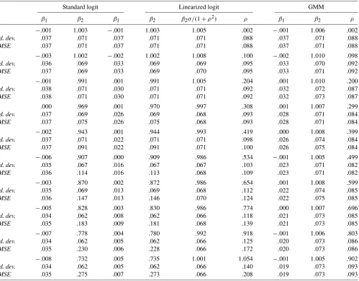
Table 1 presents the results forρ≥0 whenn=1,000. All three estimators perform well when spatial effects are absent (ρ=0). The RMSEs for both β1 andβ2 are identical in this case for each estimator. As ρ increases, standard logit fares worse than the other two estimators. Whereas the estimated values of the intercept term β1 fall slightly below their true value of zero asρincreases, the estimated values ofβ2decline markedly, averaging .732 whenρ=.9, significantly below the true value of 1. The linearized logit estimator does not correct this tendency toward a downward bias inβˆ2; the RMSEs for bothβ1andβ2are approximately the same for the standard and the linearized logit estimators. However, the linearized logit es-timator is very successful in identifying spatial effects. For val-ues ofρ between .1 and .5, the linearized logit estimates ofρ
are close to their actual values. Asρ increases, the linearized logit estimates ofρ tend to be higher than their actual values. The GMM estimator is very accurate for all values ofρ.
The downward bias in the linearized logit estimates of β2 does not automatically imply a downward bias to the marginal effects, ∂P/∂x. The probability P is a function of the index valueX∗∗β=(I−ρW)−1X∗β, andX∗is also a function ofρ
becauseX∗i =Xi/σi. In general, calculating∂Xi∗∗β/∂Xirequires some matrix manipulation. Given our experimental design,
X∗∗β=(I+ρW+ρ2W2+ρ3W3)X∗β tion, then, is whether linearized logit provides good estimates of this expression. To adjust the linearized logit estimate ofβ2, we calculateβˆ2σ/(1+.5ρ2), whereσ2is the implied value of the variance for 3<i<n−2.
The adjusted values of βˆ2 are presented for the linearized logit estimates in Table 1. The estimated values are quite ac-curate. The RMSEs for the adjusted linearized logit estimates
β2σ/(1+.5ρ2)are actually lower than the GMM estimates of
β2due to relatively low standard deviations. Of course, in gen-eral the adjusted estimates require the inversion of large matri-ces, and avoiding these calculations is one of the attractions of linearized logit over GMM estimation. Nonetheless, the matri-ces only have to be inverted once for the linearized logit estima-tor, and reasonably accurate estimates ofρare provided without having to invert a single matrix.
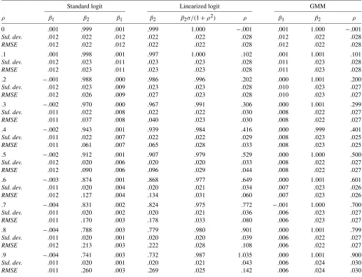
Table 2 repeats the Monte Carlo analysis for a larger sample size,n=10,000. Standard logit estimates ofβ2continue to be biased toward zero. The linearized logit estimates ofρare fairly accurate forρ≤.5, with an upward bias showing up at high values. It is important to note that the upward bias isnotevident when ρ is equal to or close to zero. Thus, the linearized logit estimator can be used to test for spatial effects without biasing the results toward rejection of the null of ρ=0. Though the
Table 1. Monte Carlo results:n=1,000
Standard logit Linearized logit GMM
ρ β1 β2 β1 β2 β2σ/(1+ρ2) ρ β1 β2 ρ
0 −.001 1.003 −.001 1.003 1.005 .002 −.001 1.006 .002
Std. dev. .037 .071 .037 .071 .071 .088 .037 .071 .088
RMSE .037 .071 .037 .071 .071 .088 .037 .071 .088
.1 −.003 1.002 −.002 1.002 1.008 .100 −.002 1.010 .098
Std. dev. .036 .069 .033 .069 .069 .095 .033 .070 .092
RMSE .037 .069 .033 .069 .070 .095 .033 .071 .092
.2 −.001 .991 .001 .991 1.005 .204 .001 1.010 .200
Std. dev. .038 .071 .030 .071 .071 .092 .032 .072 .087
RMSE .038 .071 .030 .071 .071 .092 .032 .073 .087
.3 .000 .969 .001 .970 .997 .308 .001 1.007 .299
Std. dev. .037 .069 .026 .069 .068 .093 .028 .071 .084
RMSE .037 .075 .026 .075 .068 .093 .028 .071 .084
.4 −.002 .943 .001 .944 .993 .419 .000 1.008 .399
Std. dev. .037 .071 .022 .071 .071 .098 .026 .074 .084
RMSE .037 .091 .022 .091 .071 .100 .026 .075 .084
.5 −.006 .907 .000 .909 .986 .534 −.001 1.005 .499
Std. dev. .035 .067 .016 .067 .067 .103 .023 .071 .082
RMSE .036 .114 .016 .113 .068 .109 .023 .071 .082
.6 −.003 .870 .002 .872 .986 .654 .001 1.008 .599
Std. dev. .035 .069 .013 .069 .068 .112 .022 .074 .085
RMSE .036 .147 .013 .146 .070 .124 .022 .075 .085
.7 −.005 .828 .003 .830 .986 .774 .000 1.007 .696
Std. dev. .034 .062 .008 .062 .066 .118 .021 .073 .085
RMSE .035 .183 .009 .181 .068 .139 .021 .073 .085
.8 −.007 .778 .004 .780 .992 .918 −.001 1.006 .803
Std. dev. .034 .062 .005 .062 .066 .125 .020 .073 .086
RMSE .035 .230 .006 .228 .066 .172 .020 .073 .086
.9 −.008 .732 .005 .735 1.001 1.054 −.001 1.005 .902
Std. dev. .034 .062 .005 .062 .066 .140 .019 .073 .093
RMSE .035 .275 .007 .273 .066 .208 .019 .073 .093
NOTE: Averages are calculated for 1,000 replications of a Monte Carlo experiment withβ1=0 andβ2=1.
downward bias in the linearized logit estimates ofβ2 is clear again, the adjusted estimates βσ/(1+ρ2)are quite accurate. The RMSEs of the GMM and linearized logit estimates ofρare about the same forρ < .3, but the RMSE of the GMM estimates remains low asρincreases whereas the linearized logit RMSE increases as a result of the bias inρˆ.
5. EMPIRICAL APPLICATION—DATA
North American auto supplier plants have been remarkably concentrated for a long time (Klier 2004; Klier and McMillen 2006). However, since the mid-1970s the spatial configuration of the industry has been changing (Rubenstein 1992). Whereas the industry was quite concentrated in a corridor running from Chicago to New York, it now has a north–south orientation. The industry continues to be very spatially concentrated (Ellison and Glaeser 1997). Using county-level data, Woodward (1992) and Smith and Florida (1994) found evidence that vertical link-ages as well as the presence of highway infrastructure influence plant location decisions of Japanese plants in the United States. In our empirical application, we model the location decisions of
new auto supplier plants using logit models that take explicit ac-count of the tendency for auto plants to cluster together. Despite the rapid change in the geographic configuration of the indus-try, we show that three salient features remain the same. First, Detroit remains the hub of the auto corridor, which now ex-tends southward to Kentucky and Tennessee with fingers reach-ing into Mexico and Canada. Second, both supplier plants and assembly plants tend to cluster together. Third, plant locations seldom stray far from the network of highways running toward Detroit.
We base our analysis on data acquired from ELM Inter-national, a Michigan-based vendor that attempts to cover the entire North American auto supplier industry. Data are avail-able at the plant and company level. However, plants produc-ing primarily for the aftermarket are not part of the database; nor are plants that produce machine tools or raw materials, such as steel and paint. The database includes information on a plant’s address, products, employment, parts produced, cus-tomer(s), union status, and square footage. After some prepa-ration which is described in Klier and McMillen (2006), the dataset comprises 3,416 observations of auto supplier plants lo-cated in North America.
Table 2. Monte Carlo results:n=10,000
Standard logit Linearized logit GMM
ρ β1 β2 β1 β2 β2σ/(1+ρ2) ρ β1 β2 ρ
0 .001 .999 .001 .999 1.000 −.001 .001 1.000 −.001
Std. dev. .012 .022 .012 .022 .022 .028 .012 .022 .028
RMSE .012 .022 .012 .022 .022 .028 .012 .022 .028
.1 .001 .998 .001 .997 1.000 .102 .001 1.001 .101
Std. dev. .012 .023 .011 .023 .023 .028 .011 .023 .028
RMSE .012 .023 .011 .023 .023 .028 .011 .023 .028
.2 −.001 .988 .000 .986 .996 .202 .000 1.001 .200
Std. dev. .012 .023 .009 .023 .023 .028 .010 .023 .027
RMSE .012 .026 .009 .027 .023 .028 .010 .023 .027
.3 −.002 .970 .000 .967 .991 .306 .000 1.001 .299
Std. dev. .011 .022 .008 .022 .022 .030 .008 .022 .027
RMSE .011 .037 .008 .040 .023 .030 .008 .022 .027
.4 −.002 .943 .001 .939 .984 .416 .000 .999 .401
Std. dev. .011 .022 .007 .022 .022 .029 .008 .023 .025
RMSE .011 .061 .007 .065 .028 .033 .008 .023 .025
.5 −.002 .912 .001 .907 .979 .529 .000 1.000 .500
Std. dev. .012 .020 .006 .020 .020 .033 .008 .022 .027
RMSE .012 .090 .006 .096 .029 .044 .008 .022 .027
.6 −.003 .874 .001 .868 .977 .649 .000 1.001 .601
Std. dev. .011 .020 .004 .020 .021 .034 .007 .023 .026
RMSE .012 .127 .004 .134 .031 .060 .007 .023 .026
.7 −.004 .831 .002 .824 .975 .772 −.001 1.000 .700
Std. dev. .011 .020 .002 .020 .021 .036 .006 .023 .027
RMSE .011 .170 .003 .178 .033 .080 .006 .023 .027
.8 −.004 .788 .003 .779 .980 .901 .000 1.001 .799
Std. dev. .011 .020 .001 .020 .020 .039 .006 .022 .027
RMSE .012 .213 .003 .222 .028 .108 .006 .022 .027
.9 −.004 .741 .003 .732 .987 1.035 .000 1.001 .900
Std. dev. .011 .020 .001 .020 .021 .043 .006 .024 .030
RMSE .011 .260 .003 .269 .025 .142 .006 .024 .030
NOTE: Averages are calculated for 10,000 replications of a Monte Carlo experiment withβ1=0 andβ2=1.
Our analysis focuses on new plants—those that opened be-tween 1991 and 2003. Focusing on new plants has several ad-vantages. First, it allows us to determine whether recent plant location decisions differ from those of the past. The Ameri-can auto industry went through major changes in the 1980s as Japanese producers opened U.S. plants and the entire industry moved toward a north–south orientation about its Detroit base. Focusing on new plants allows us to determine the extent to which agglomerative forces have changed over time. A second advantage of focusing on plant openings from after 1990 is that it allows us to match the plant openings with explanatory vari-ables from the 1990 U.S. Census. Moving the date forward by one year from the time of the Census ensures that these explana-tory variables can be taken as exogenous. Third, focusing on new plants helps to avoid survivor bias. In this cross-sectional dataset, the age variable applies only to surviving establish-ments. This focus on survivors could lead us to understate the extent to which “old” plants are concentrated at the upper end of the auto corridor. Survivor bias is much less of a problem when focusing on new plant sites.
Another advantage of focusing on new plants is that it al-lows us to avoid potential endogeneity problems when
analyz-ing agglomeration. Explanatory variables for new plant loca-tions include the number of nearby assembly and existing sup-plier plants. Because existing supsup-plier plants date from prior to 1991, their spatial distribution can be taken as exogenous. We also treat the location of assembly plants during the ob-servation period as exogenous. Only eight assembly plants were opened between 1991 and 2003 (these plants represent 13% of all assembly plants operational in the United States in 2003). With most assembly plant locations predetermined and the others opened only with long lead times, the assump-tion that assembly plant locaassump-tions are exogenous is reason-able.
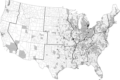
Figure 1 shows the location of existing (pre-1991) supplier plants in North America in 2003, along with the sites of as-sembly plants. The dominance of the East North Central re-gion is striking. Detroit remains the core of the industry, with large numbers of counties occupied by supplier plants in Ohio and Indiana, also. The locus of the industry has been moving southward over time. Though many plants are still evident in New England and the Middle Atlantic States, the East South Central and South Atlantic states have been adding plants re-cently. Very few plants are located in the western states.
Figure 1. Counties with existing plants.
ure 2 shows the location of supplier plants that opened between 1991 and 2003. Most of the new plants are located along a path running south from Detroit, although a respectable number of plants have opened in New England and the Middle Atlantic states. The tendency of supplier plants to locate near assemblers is clear in both Figures 1 and 2.
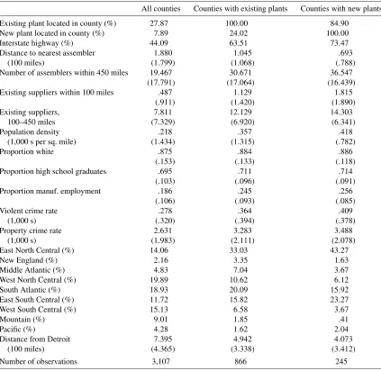
Table 3 presents descriptive statistics for the variables used in our analysis. Of the 3,107 counties in the 48 contiguous states for which all data are available, 866 (27.87%) have plants that opened before 1991 and 245 (7.89%) have new plants. Most new plants are located in counties that already have an exist-ing plant: only 37 counties have only a new plant. As shown in
Figure 2. Counties with new plants.
Table 3. Descriptive statistics
All counties Counties with existing plants Counties with new plants
Existing plant located in county (%) 27.87 100.00 84.90 New plant located in county (%) 7.89 24.02 100.00 Interstate highway (%) 44.09 63.51 73.47 Distance to nearest assembler 1.880 1.045 .693
(100 miles) (1.799) (1.068) (.788)
Number of assemblers within 450 miles 19.467 30.671 36.547
(17.791) (17.064) (16.439)
Existing suppliers within 100 miles .487 1.129 1.815
(.911) (1.420) (1.890)
Existing suppliers, 7.811 12.129 14.303 100–450 miles (7.329) (6.920) (6.341)
Population density .218 .357 .418
(1,000 s per sq. mile) (1.434) (1.315) (.782)
Proportion white .875 .884 .886
(.153) (.133) (.118)
Proportion high school graduates .695 .711 .714
(.103) (.096) (.091)
Proportion manuf. employment .186 .245 .256
(.106) (.093) (.085)
Violent crime rate .278 .364 .409
(1,000 s) (.320) (.394) (.378)
Property crime rate 2.631 3.283 3.488 (1,000 s) (1.983) (2.111) (2.078)
East North Central (%) 14.06 33.03 43.27
New England (%) 2.16 3.35 1.63
Middle Atlantic (%) 4.83 7.04 3.67
West North Central (%) 19.89 10.62 6.12 South Atlantic (%) 18.93 20.09 15.92 East South Central (%) 11.72 15.82 23.27 West South Central (%) 15.13 6.58 3.67
Mountain (%) 9.01 1.85 .41
Pacific (%) 4.28 1.62 2.04
Distance from Detroit 7.395 4.942 4.073 (100 miles) (4.365) (3.338) (3.412)
Number of observations 3,107 866 245
NOTE: Standard deviations are in parentheses for continuous variables.
Figures 1 and 2, both new and existing plants are concentrated in the East North Central, South Atlantic, and East South Cen-tral Census regions; these three regions account for more than two-thirds (32.45%, 20.16%, and 16.06%, resp.) of the counties with auto supplier plants in 2003. The rotation of the auto re-gion toward a corridor running south from Detroit is evident in the tendency for new plants to open up in the East North Cen-tral and East South CenCen-tral regions. In fact, counties with new plants tend to be closer to Detroit on average than counties with existing plants—407 miles compared to 494 miles. New sup-plier plants are also closer to assembly plants on average than are the existing suppliers: the centers of the counties in which new plants are located are 693 miles from the nearest assembler on average, compared with 1,045 miles for existing plants. The number of assembly plants within 450 miles of county centers is also higher for new plants than for existing plants—36.547 versus 30.671. Overall, Table 3 suggests that the auto industry is retrenching by drawing closer to Detroit along a north–south corridor.
The explanatory variables drawn from the Census include characteristics of the counties in which the plants opened—
population density, the proportion of the residents who are white, the proportion who have graduated from high school, the proportion of the employment in the county that is in man-ufacturing, and measures of the rates of violent and property crime. Other explanatory variables include the regional dummy variables and distance from Detroit. We include a dummy vari-able indicating whether an interstate highway runs through the county. Auto suppliers have increasingly been using just-in-time manufacturing systems, placing a premium on locations near highways running to assembly plants and to Detroit. To account for the tendency to locate near assembly plants, our ex-planatory variables include the distance to the nearest assembler and the count of the number of assemblers within 450 miles (an approximate one day’s drive) from the center of the county.
We account for the tendency of supplier plants to cluster in two ways. First, we include the spatial lag variable,WY, which is a weighted average of the propensity for neighboring coun-ties to have a supplier plant. The weight matrix,W, is a con-tiguity matrix. We construct the matrix by setting Wij=1/ni for counties that share a common border, whereni is the num-ber of observations that are contiguous to countyi.Wij=0 for
all other observations (includingWii). A positive value for this variable’s coefficient implies a county’s probability of having a plant increases with the propensity for neighboring counties to have plants. Our second measure of the tendency to cluster is the number ofexistingsuppliers (as of 1990) within 100 miles and between 100 and 450 miles of the center of the county. The results for these variables will help determine whether the lo-cation decisions for new plants simply mimic those of existing plants.
GMM estimation is impractical for the full sample of 3,107 counties. In order to compare the linearized logit estimates to GMM, we employ a simplifying assumption that significantly reduces computation time for matrix inversions. For GMM es-timation, we alter the weight matrix such that Wij=0 when countiesiandjare in different Census regions. This assump-tion greatly reduces computaassump-tional time by producing a block
diagonal structure forW. Although computational time could be reduced still further if we used states rather than Census re-gions as the basis for the blocks, the advantage of using Census regions is that the resulting weight matrix is closer to the orig-inal structure in whichW is not block diagonal. Comparisons of linearized logit estimates for the original specification ofW
and the block diagonal specification suggest that the results are very similar.
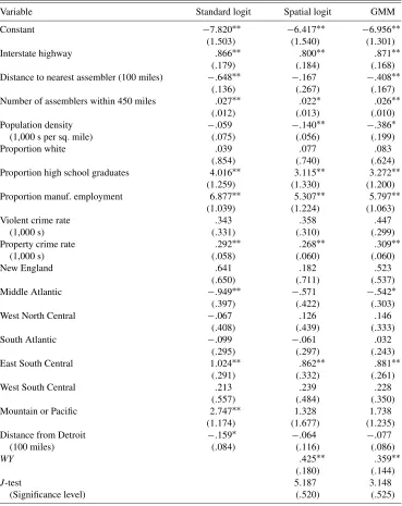
6. LOGIT RESULTS
Our base model for counties with new plants is shown in the first column of results in Table 4. The estimated logit model in-dicates that the presence of an interstate highway significantly increases the probability that a county will have a new auto sup-plier plant. The probability of having a new plant also increases
Table 4. Logit models for new supplier plants: No controls for location of existing suppliers
Variable Standard logit Spatial logit GMM
Constant −7.820∗∗ −6.417∗∗ −6.956∗∗
(1.503) (1.540) (1.301)
Interstate highway .866∗∗ .800∗∗ .871∗∗
(.179) (.184) (.168)
Distance to nearest assembler (100 miles) −.648∗∗ −.167 −.408∗∗
(.136) (.267) (.167)
Number of assemblers within 450 miles .027∗∗ .022∗ .026∗∗
(.012) (.013) (.010)
Population density −.059 −.140∗∗ −.386∗ (1,000 s per sq. mile) (.075) (.056) (.199)
Proportion white .039 .077 .083
(.854) (.740) (.624)
Proportion high school graduates 4.016∗∗ 3.115∗∗ 3.272∗∗
(1.259) (1.330) (1.200)
Proportion manuf. employment 6.877∗∗ 5.307∗∗ 5.797∗∗
(1.039) (1.224) (1.063)
Violent crime rate .343 .358 .447
(1,000 s) (.331) (.310) (.299)
Property crime rate .292∗∗ .268∗∗ .309∗∗
(1,000 s) (.058) (.060) (.060)
New England .641 .182 .523
(.650) (.711) (.537)
Middle Atlantic −.949∗∗ −.571 −.542∗
(.397) (.422) (.303)
West North Central −.067 .126 .146
(.408) (.439) (.333)
South Atlantic −.099 −.061 .032
(.295) (.297) (.243)
East South Central 1.024∗∗ .862∗∗ .881∗∗
(.291) (.332) (.261)
West South Central .213 .239 .228
(.557) (.484) (.350)
Mountain or Pacific 2.747∗∗ 1.328 1.738
(1.174) (1.677) (1.235)
Distance from Detroit −.159∗ −.064 −.077
(100 miles) (.084) (.116) (.086)
WY .425∗∗ .359∗∗
(.180) (.144)
J-test 5.187 3.148
(Significance level) (.520) (.525)
NOTE: Standard errors are in parentheses. Significance at the 5% and 10% level is indicated by “**” and “*.”
if the center of the county is close to an assembly plant and if it is within a day’s drive from a large number of assemblers. Not surprisingly, the probability of having a new supplier plant is higher if the county has a high proportion of high school gradu-ates and if it already has a high concentration of manufacturing employment. A somewhat surprising result is our finding that the probability of having a plant is higher in counties with high crime rates. This result holds even though we have controlled for the population density in the counties. A possible expla-nation is that high crime rates reduce land values in a county, and that auto plants substitute toward private security provision. Another possibility is that crime rates are correlated with urban locations in a way that is not captured by the population density variable. At any rate, the positive association between crime and plant location is a robust result that holds up in subsequent models.
The auto industry has traditionally been clustered in the base location, the East North Central region. Evidence that the in-dustry is moving from an east–west to a north–south orienta-tion is provided by the significantly negative coefficient for the Middle Atlantic region and the positive coefficient for the East South Central region. (The Mountain and Pacific regions were combined due to the small number of plants in these locations.) Although distance from Detroit is not a significant determinant of plant locations once other variables are taken into account, plants are much more likely to be located near assembly plants and in counties containing interstate highways. Because assem-bly plants are clustered in the auto corridor around Detroit, sup-plier plants tend to cluster together also.
The results for the linearized spatial logit model and GMM estimator are also presented in Table 4. Instruments for the GMM estimation procedure include all of the exogenous vari-ables shown in Table 4. In addition, we include the weighted average of nearby values (WX) of those variables that vary sig-nificantly over space—the presence of an interstate highway, population density, crime rates, the proportion of employment that is in manufacturing, and the proportions of the county’s residents who are white and who have high school degrees. We test for the statistical validity of the instruments using Hansen’s (1982)J-test. TheJ-test simultaneously tests the overall model specification and the potential endogeneity of the instruments.
Most of the results for the spatial version of the model are quite similar to those for the standard model. The main dif-ference is simply the significance of the spatial lag variable (WY). The positive coefficient forWYimplies that the probabil-ity that a county has an existing supplier plant increases when neighboring counties have a high propensity to have plants as well. These results suggest that existing plants cluster together closely, even beyond the extent indicated by the controls for re-gions, the presence of nearby assembly plants, highways, and other manufacturing establishments.
The spatial logit and GMM estimates ofρare similar in Ta-ble 4, .425 versus .359. The standard error is lower for GMM estimation, but both estimators strongly reject the null ofρ=0. In general, the coefficients are similar across the two spatial models even though the estimates are not adjusted for the bias found in the Monte Carlo study. However, standard errors are lower for the GMM estimator. TheJ-test does not reject the validity of the instruments for either estimator.
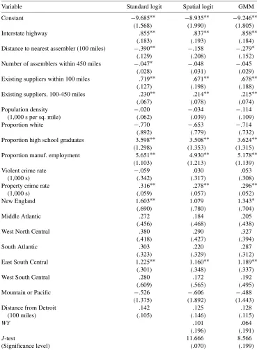
Table 5 adds two variables to the models, the number of existing suppliers within 100 miles and between 100 and 450 miles of the county. The probability of having a new plant in a county rises significantly when older plants already exist in the area, with a pronounced effect if there already are plants within 100 miles of the county center. Although the effect di-minishes in size for plants located within the larger radius, it re-mains statistically significant. The spatial autoregressive term is no longer statistically significant once these variables are added to the models. Though new plants have a tendency to cluster to-gether, the tendency simply mimics the location pattern of ex-isting plants. There is no increment to the clustering tendency among new plants. As in Table 4, the linearized logit and GMM results are generally similar, and the J-test does not reject the validity of the instruments.
7. CONCLUSION
The spatial autoregression model is useful when individual decisions are mutually dependent and are influenced by prox-imity. Do tax rates in one jurisdiction depend on tax rates in nearby jurisdictions? Does the presence of growth controls de-pend on whether neighboring municipalities have growth con-trols? Does the sales price of a house depend on the prices paid for nearby homes? We show that the same class of model is use-ful for identifying clustering in the location decisions of auto supplier plants in the United States. Does the presence of sup-plier plants in neighboring counties increase the probability that a county will also have a plant? We find strong evidence of clus-tering among new auto supplier plants. New supplier plants are more likely to locate in counties that are near assembly plants, in counties that contain a stretch of interstate highway, and in counties that already have supplier plants. But whereas new plants tend to cluster, there is no additional tendency toward clustering beyond that shown by older plants.
We extend the literature on spatial modeling in two ways. First, we extend the standard spatial autoregression model to the case of a discrete variable. Our model is appropriate if thepropensity to have a value of 1 for the dependent variable depends on the propensity for nearby observations. Thus, the probability that an auto supplier plant is located in a county de-pends on the underlying latent variable determining the proba-bility that nearby counties have assembly and/or supplier plants. The model can be estimated using a straightforward extension of the GMM estimator proposed by Pinkse and Slade (1998) for a spatial model. Our second contribution to the literature on spatial modeling is to show how a linearized version of the GMM approach can be used to estimate the spatial logit model when the sample size is large.
Monte Carlo estimates suggest that the linearized logit es-timator is very accurate at identifying spatial effects. When
ρ > .5, the estimates of the spatial parameter are biased upward, but whenρis close to zero there is no bias. Combining the lin-earized logit estimates with a single calculation of(I−ρW)−1
produces very accurate estimates of(I−ρW)−1X∗β. Our em-pirical application suggests that the linearized model’s esti-mates are very similar to full GMM estiesti-mates. However, the computational burden of full GMM estimation can be pro-hibitive in even moderately sized samples, whereas the lin-earized model requires two simple steps—standard logit and
Table 5. Logit models for new supplier plants: No controls for location of existing suppliers
Variable Standard logit Spatial logit GMM
Constant −9.685∗∗ −8.935∗∗ −9.246∗∗
(1.568) (1.990) (1.805)
Interstate highway .855∗∗ .837∗∗ .858∗∗
(.183) (.193) (.184)
Distance to nearest assembler (100 miles) −.390∗∗ −.158 −.279∗
(.129) (.208) (.152)
Number of assemblers within 450 miles −.047∗ −.048 −.045
(.028) (.031) (.029)
Existing suppliers within 100 miles .719∗∗ .671∗∗ .678∗∗
(.127) (.198) (.188)
Existing suppliers, 100-450 miles .230∗∗ .214∗∗ .215∗∗
(.067) (.078) (.074)
Population density −.020 −.034 −.114 (1,000 s per sq. mile) (.062) (.039) (.109)
Proportion white −.770 −.653 −.714
(.892) (.779) (.732)
Proportion high school graduates 3.598∗∗ 3.508∗∗ 3.624∗∗
(1.298) (1.353) (1.315)
Proportion manuf. employment 5.651∗∗ 4.930∗∗ 5.178∗∗
(1.103) (1.213) (1.139)
Violent crime rate −.059 .030 .053
(1,000 s) (.342) (.317) (.308)
Property crime rate .316∗∗ .278∗∗ .296∗∗
(1,000 s) (.059) (.057) (.052)
New England 1.603∗∗ 1.079 1.343∗
(.690) (.780) (.704)
Middle Atlantic .272 .184 .205
(.456) (.468) (.438)
West North Central .380 .290 .327
(.418) (.427) (.394)
South Atlantic .303 .220 .287
(.323) (.329) (.312)
East South Central 1.225∗∗ 1.160∗∗ 1.189∗∗
(.301) (.348) (.337)
West South Central .280 .172 .192
(.609) (.565) (.495)
Mountain or Pacific −.526 −.606 −.488
(1.375) (1.892) (1.443)
Distance from Detroit .142 .125 .128
(100 miles) (.105) (.146) (.115)
WY .101 .064
(.196) (.191)
J-test 11.666 8.566
(Significance level) (.070) (.199)
NOTE: Standard errors are in parentheses. Significance at the 5% and 10% level is indicated by “**” and “*.”
two-step least squares. The tractability of the linearized logit estimator makes it a very attractive option for large datasets.
ACKNOWLEDGMENT
The authors thank Cole Bolton and Paul Ma for excellent research assistance.
[Received May 2005. Revised January 2007.]
REFERENCES
Anselin, L. (1988),Spatial Econometrics, Boston: Kluwer Academic Publish-ers.
Beron, K. J., and Vijverberg, W. P. M. (2004), “Probit in a Spatial Context: A Monte Carlo Analysis,” inAdvances in Spatial Econometrics: Methodol-ogy, Tools and Applications, eds. L. Anselin, R. J. G. M. Florax, and S. J. Rey, New York: Springer, pp. 169–195.
Bordignon, M., Cerniglia, F., and Revelli, F. (2003), “In Search of Yardstick Competition: Property Tax Rates and Electoral Behavior in Italian Cities,” Journal of Urban Economics, 54, 199–217.
Brett, C., and Pinkse, J. (2000), “The Determinants of Municipal Tax Rates in British Columbia,”Canadian Journal of Economics, 33, 695–714. Brueckner, J. K. (1998), “Testing for Strategic Interaction Among Local
Gov-ernments: The Case of Growth Controls,”Journal of Urban Economics, 44, 438–467.
(2003), “Strategic Interaction Among Governments: An Overview of Empirical Studies,”International Regional Science Review, 26, 175–188. Brueckner, J. K., and Saavedra, L. A. (2001), “Do Local Governments Engage
in Strategic Property-Tax Competition?”National Tax Journal, 54, 203–229.
Case, A. C. (1992), “Neighborhood Influence and Technological Change,” Re-gional Science and Urban Economics, 22, 491–508.
Case, A. C., Rosen, H. S., and Hines, J. C. (1993), “Budget Spillovers and Fiscal Policy Interdependence: Evidence From the States,”Journal of Public Economics, 52, 285–307.
Ellison, G., and Glaeser, E. L. (1997), “Geographic Concentration in U.S. Man-ufacturing Industries: A Dartboard Approach,”Journal of Political Economy, 105, 889–927.
Flores-Lagunes, A., and Schnier, K. E. (2005), “Estimation of Sample Selection Models With Spatial Dependence,” working paper, University of Arizona. Fredriksson, P. G., and Millimet, D. L. (2002), “Strategic Interaction and the
Determinants of Environmental Policy Across U.S. States,”Journal of Urban Economics, 51, 101–122.
Greene, W. H. (2002),Econometric Analysis, Upper Saddle River, NJ: Prentice-Hall.
Hansen, L. P. (1982), “Large Sample Properties of Generalized Method of Mo-ments Estimators,”Econometrica, 50, 1029–1054.
Harbour Consulting (2003),Harbour Report, 2004.
Kelijian, H. H., and Prucha, I. R. (1998), “A Generalized Spatial Two-Stage Least Squares Procedure for Estimating a Spatial Autoregressive Model With Autoregressive Disturbances,”Journal of Real Estate Finance and Eco-nomics, 17, 99–121.
Klier, T. (2004), “Challenges to the U.S. Auto Industry,” Chicago Fed Letter, Chicago: Federal Reserve Bank of Chicago.
Klier, T., and McMillen, D. P. (2006), “The Geographic Evolution of the U.S. Auto Industry,”Economic Perspectives, 30, 2–13.
LeSage, J. P. (2000), “Bayesian Estimation of Limited Dependent Variable Spa-tial Autoregressive Models,”Geographical Analysis, 32, 19–35.
McMillen, D. P. (1992), “Probit With Spatial Autocorrelation,”Journal of Re-gional Science, 32, 335–348.
(1995), “Spatial Effects in Probit Models: A Monte Carlo Investiga-tion,” inNew Directions in Spatial Econometrics, eds. L. Anselin and R. J. G. M. Florax, New York: Springer-Verlag, pp. 189–228.
Pinkse, J., and Slade, M. E. (1998), “Contracting in Space: An Application of Spatial Statistics to Discrete-Choice Models,”Journal of Econometrics, 85, 125–154.
Revelli, F. (2003), “Reaction or Interaction: Spatial Process Identification in Multi-Tiered Governmental Structures,”Journal of Urban Economics, 53, 29–53.
Rubenstein, J. M. (1992),The Changing U.S. Auto Industry—A Geographical Analysis, London: Routledge.
Saavedra, L. A. (2000), “A Model of Welfare Competition With Evidence From AFDC,”Journal of Urban Economics, 47, 248–279.
Smith, D., and Florida, R. (1994), “Agglomeration and Industrial Location: An Econometric Analysis of Japanese-Affiliated Manufacturing Establishments in Automotive-Related Industries,”Journal of Urban Economics, 36, 23–41. Woodward, D. (1992), “Locational Determinants of Japanese Manufacturing Start-Ups in the United States,”Southern Economic Journal, 58, 690–708.