Full Terms & Conditions of access and use can be found at
http://www.tandfonline.com/action/journalInformation?journalCode=ubes20
Download by: [Universitas Maritim Raja Ali Haji] Date: 13 January 2016, At: 00:33
Journal of Business & Economic Statistics
ISSN: 0735-0015 (Print) 1537-2707 (Online) Journal homepage: http://www.tandfonline.com/loi/ubes20
Bayesian Analysis of Interval Data Contingent
Valuation Models and Pricing Policies
Carmen Fernández, Carmelo J León, Mark F.J Steel & Francisco José
Vázquez-Polo
To cite this article: Carmen Fernández, Carmelo J León, Mark F.J Steel & Francisco José
Vázquez-Polo (2004) Bayesian Analysis of Interval Data Contingent Valuation Models and Pricing Policies, Journal of Business & Economic Statistics, 22:4, 431-442, DOI: 10.1198/073500104000000415
To link to this article: http://dx.doi.org/10.1198/073500104000000415
View supplementary material
Published online: 01 Jan 2012.
Submit your article to this journal
Article views: 52
Bayesian Analysis of Interval Data Contingent
Valuation Models and Pricing Policies
Carmen F
ERNÁNDEZDepartment of Mathematics and Statistics, Lancaster University, Lancaster, U.K. (c.fernandez@lancaster.ac.uk)
Carmelo J. L
EÓNDepartment of Applied Economic Analysis, University of Las Palmas de Gran Canaria, Las Palmas de Gran Canaria, Spain (cleon@daea.ulpgc.es)
Mark F. J. S
TEELDepartment of Statistics, University of Warwick, Coventry, U.K. (m.f.steel@stats.warwick.ac.uk)
Francisco José V
ÁZQUEZ-P
OLODepartment of Quantitative Methods, University of Las Palmas de Gran Canaria, Las Palmas de Gran Canaria, Spain (fjvpolo@dmc.ulpgc.es)
The general aim of a contingent valuation survey is to elicit the willingness to pay (WTP) of respondents for some (public) commodity without a clear market price. This could be a program to protect some environmental resource or, as in our application, the access to a recreational area of particular interest. In this context, we want to accommodate the possibility of zero WTP and we need to deal with the fact that observations arise as intervals for WTP, rather than point observations. We propose a flexible Bayesian statistical analysis of WTP as a function of characteristics of the respondents that formally incorporates this structure through a mixture model. We consider model uncertainty and pay particular attention to the predictive distribution of revenue if a certain entry price were asked. The latter is an important tool for deriving pricing policies.
KEY WORDS: Dichotomous choice; Ignorability; Mount Teide National Park; Posterior existence; Revenue; Willingness to pay.
1. INTRODUCTION
Contingent valuation (CV) surveys aim to elicit the willing-ness to pay (WTP) of respondents for some good not currently marketed. A guide to the basic techniques has been provided by Mitchell and Carson (1989), and a recent overview has been given by Carson, Flores, and Meade (2001). The CV methodol-ogy has been applied to a wide array of problems in the val-uation of public goods, including those whose value largely comes from existence rather than active use (such as endan-gered species or wilderness areas). The same ideas are now also widely applied in the context of health care, as done by Blumenschein, Johannesson, Yokoyama, and Freeman (2001). The CV survey data analyzed in this article were collected with the purpose of appraising the WTP to enter the Teide National Park (Canary Islands, Spain) among the population of poten-tial visitors. The park receives 3 million visitors per year, and entrance is currently free. The main motivation for the study is the extraction of consumer surplus from visitors, particularly foreign visitors. There is interest in a relevant (possibly differ-ential) pricing policy to transfer the benefits that visitors expe-rience to the local population.
In a CV survey, a random sample of individuals are asked to answer a questionnaire containing a hypothetical market trans-action with the purpose of eliciting their WTP for obtaining a good or their willingness to accept (WTA) compensation for giving up a good. WTP is the appropriate measure for our appli-cation, and we will use it in the sequel. In this paper we develop Bayesian methods for estimating WTP models from CV survey data, focusing on the so-called “double-bounded dichotomous-choice” elicitation format.
Double-bounded surveys involve two binary questions cor-responding to two successive bid prices. First, the individual receives a random bid, which is subsequently raised or lowered depending on the initial response. Combining the responses to both questions leads to (bounded or unbounded) intervals for WTP. This method has been shown to increase statistical efficiency with respect to the single-bounded method where the individual is offered only one bid (see Hanemann, Loomis, and Kanninen 1991; Cameron and Huppert 1991). Models for these kinds of data have been estimated with maximum likeli-hood methods, (e.g., Hanemann et al. 1991). Despite its sta-tistical efficiency, the double-bounded format has sometimes been subject to criticism (see, e.g., Herriges and Shogren 1996 and Alberini 1995 for opposing sides of this debate), which prompted the so-called “one-and-one-half-bound” approach of Cooper, Hanemann, and Signorello (2002), leading to a lower proportion of bounded intervals. Our methodology can also be applied to this alternative format.
To our knowledge, Bayesian inference for CV survey inter-val data has not been conducted to date. The analysis devel-oped here formally takes the interval nature of the data into account and also allows for a proportion of the population to have zero WTP. Our model for WTP is a mixture model, with a point mass at 0 modeled through a probit model, whereas the part corresponding to positive WTP is of a log-linear form with possibly skewed and fat-tailed distributions. Thus our
model-© 2004 American Statistical Association Journal of Business & Economic Statistics October 2004, Vol. 22, No. 4 DOI 10.1198/073500104000000415
431
ing framework introduces a substantial amount of flexibility, accounting for a variety of valuation distributions, and we use Bayes factors to select the best among them (or to average over them, if preferred).
This article contributes to the development of Bayesian meth-ods for CV data in the following four ways. First, inference is conducted on the parameters explaining WTP, allowing for the incorporation of covariates; second, a flexible class of distrib-utions is assumed, specifically intended to model a wide range of valuation behavior; third, zero WTP is treated accordingly in the model and inference process; and finally, the predictive distribution of WTP is analyzed and used to predict revenue in a pricing context. The classical counterpart of the Bayesian predictive distribution often consists of the sampling distrib-ution with the parameter estimates plugged in. This ignores the uncertainty about the parameters and distributional mod-els and thus typically underestimates uncertainty. Most existing CV studies focus on summarizing the WTP distribution (usu-ally mean WTP, but occasion(usu-ally median WTP), rather than ex-amining the entire distribution. However, working on the basis of the entire predictive distribution of WTP is preferable, be-cause it contains all inference regarding WTP, which can then be used appropriately (as we illustrate in the context of price-setting in Sec. 4).
The article is organized as follows. In Section 2 we carefully look at the structure of the data and establish that the double-bounded elicitation procedure can be ignored in writing down the likelihood; in addition, we present the specification of the sampling and prior distributions. In Section 3 we deal with var-ious properties of the Bayesian method, including how to com-pute Bayes factors to discriminate among competing models involving different distributional assumptions. In this section we also discuss posterior propriety under an improper non-informative prior and sketch the Markov chain Monte Carlo (MCMC) sampler for posterior inference. In Section 4 we ex-plore the predictive distributions of WTP and revenue as an instrument for pricing decisions. We focus particularly on re-sults that are representative of the entire target population rather than on those for individuals with particular values of the co-variates; however, the same strategy could be applied to cer-tain subgroups of individuals (e.g., foreign visitors), and price discrimination fits naturally into our framework. In Section 5 we describe the empirical Teide National Park data application in detail, and in Section 6 we present the main findings of the analysis, obtaining, among other results, the optimal (in terms of expected revenue maximization) entry fee for Teide National Park. We provide some concluding remarks in Section 7, and group all proofs in the Appendix.
2. DATA STRUCTURE AND STATISTICAL MODEL
2.1 The Structure of the Data
The CV survey that we focus on in this study leads to a par-ticular data format. The survey is conducted as follows. First, the individual is offered a price (or bid) and answers whether he or she is willing to pay this amount. If the answer is yes, then he or she is offered a higher price and the answer to that is also recorded. In the case of a negative answer to the first price, a lower price is offered.
If both answers are negative, then the individual is asked whether he or she is not willing to pay anything at all (and the reason for the zero WTP when this is stated). This makes it possible to distinguish between having a WTP that is positive but lower than the lowest bid offered and having zero WTP. Loomis, Traynor, and Brown (1999) introduced a trichotomous choice format that explicitly allows for zero WTP. The zero re-sponses could reflect a refusal to adopt a market context for the good. In our application, most zero respondents felt they should not be charged for entering natural areas in general.
We work under the assumption that each person has a single maximum WTP that is not affected by the questions asked and that the person answers in accordance with this WTP. Thus, for a number of individuals we observe zero WTP, whereas for the remaining individuals (who must therefore have a posi-tive WTP), we obtain an observation of WTP in the form of an interval, which can be either bounded or unbounded.
The bids offered to the individuals surveyed are generated according to some (typically random) scheme. In the following proposition, we show that, under very general conditions, the way in which the bids are generated does not affect the way in which inference is conducted.
Proposition 1. For each individual in the survey, assume the following:
a. The value of the first bid is generated from some proba-bility distribution.
b. The value of the second bid is generated from a probabil-ity distribution that depends only on the value of the first bid and the individual’s (yes/no) answer to it.
Then the mechanism that generates the bids can be ignored when conducting likelihood-based inference on the WTP dis-tribution.
We note that Proposition 1 also covers the case in which one or both of the probability distributions used to generate the bids is a point mass (i.e., nonrandom). For example, in our specific survey, the first bid is offered to the subject following a uni-form discrete distribution in a prespecified finite set of values, whereas the value of the second bid is completely determined by the value of the first bid and the individual’s response to it.
Proposition 1 implies that we can work with our data as if they are interval observations from the individuals’ WTP dis-tributions and we can ignore the double-bounded elicitation mechanism. Ignorability of the data-coarsening mechanism was studied, in a general setting, by Heitjan and Rubin (1991). Our result applies to any likelihood-based inference, so it covers both classical (e.g., maximum likelihood) and Bayesian meth-ods.
2.2 The Model for Willingness to Pay
In our context, it seems natural to assume that WTP is non-negative and that a certain fraction of the relevant population has a zero WTP. Thus we consider a model for WTP
consist-ing of a positive probability attached to WTP=0 and, with
the remaining probability, some continuous distribution over the positive real line. Several possibilities have been proposed in the literature. Some authors have modeled WTP via a con-tinuous distribution over the entire real line, but assuming that
WTP is observed only over the positive real line. In that case, a response WTP=0 could be interpreted as a censored obser-vation meaning, in reality, that WTP≤0. Models of this form have been used by Kriström (1997) and Loomis et al. (1999), among others. A natural extension is to model the probability
that WTP=0 separately from the continuous distribution of
WTP over the positive real line. The spike models of Kriström (1997) allow for this possibility, and the mixture models of Werner (1999) and Reiser and Shechter (1999) (the latter in a single bounded CV context) are of this form. These models are more natural than censored models when it is felt that a zero
re-sponse genuinely means that WTP=0 as opposed to meaning
that WTP≤0, and when the reasons that lead people to have a zero WTP could differ from the reasons that give them a partic-ular positive value of WTP. The latter value is often influenced by budgetary considerations, whereas in our application, most zero WTP respondents stated that they felt that entrance to nat-ural areas should be free as a matter of principle. Thus we have decided to use a general mixture model. In addition to WTP, our CV survey records a number of characteristics for each individ-ual interviewed, and we take these into account when building our model. Our modeling strategy is thus quite similar to that of Werner (1999) and Reiser and Shechter (1999), although the actual model implemented, the inferential procedure, and the way in which the results are put to practice are quite different.
Denoting by wi the WTP of the ith individual, a mixture
model corresponds to a cumulative distribution function (cdf ) of the form
positive real line describing the distribution of positive WTP. In this article we consider a probit model, and thus
pi=P(wi>0)=(z′iδ), (2)
where (·) denotes the cdf of the standard normal distribu-tion. The vector zi contains the element 1 as well as m−1
explanatory variables chosen from the available individual char-acteristics, andδ∈Rmgroups the intercept and the regression
coefficients. The covariate vector zi can contain both
contin-uous and categorical variables, where the latter are handled through dummies with one level excluded.
We now turn to the choice of Fi(·)in (1). Ifwi is positive,
then its level will be modeled via log-linear regression, using a vectorxicontaining a unitary element andk−1 individual
co-variates (again selected from the set of individual characteristics observed in the survey). In particular, we defineyi=log(wi)
and assume that
yi=x′iβ+σ εi, (3)
where theεi are iid random variables onR. In (3) we have
in-troduced the scale parameterσ >0 and the regression vector
β∈Rk. The most common choices for the distribution ofεiin
the literature are normal (see, e.g., Cameron and Huppert 1991) and logistic. Buckland, Macmillan, Duff, and Hanley (1999) considered logistic models on various transformations of WTP in the single-bounded context. Hanemann and Kanninen (1999) have provided an extensive survey. In this article, we take the normal distribution as our starting point, but we consider a more
flexible framework to account for a variety of valuation distrib-utions, using the ideas proposed by Fernández and Steel (1998). In particular, we consider the following densities forεi:
p(εi|γ )=
whereI[·]denotes the indicator function. The pdf in (4) is that of a skewed normal, whereγ >0 is the skewness parameter, controlling the mass allocated to both sides of the mode at 0. Values ofγ larger than unity will induce right-skewness, and forγ <1 we have left-skewness. The normal distribution is
found as the special case where γ =1. The same principle
for introducing skewness is applied to the Student-t distribu-tion in equadistribu-tion (5), which we call “skewed Student.” Again, forγ =1 (5) reduces to the Student-t distribution withν >0 degrees of freedom. Thus, (4) allows for skewness in the distri-bution of log(WTP),yi, whereas (5) accommodates both
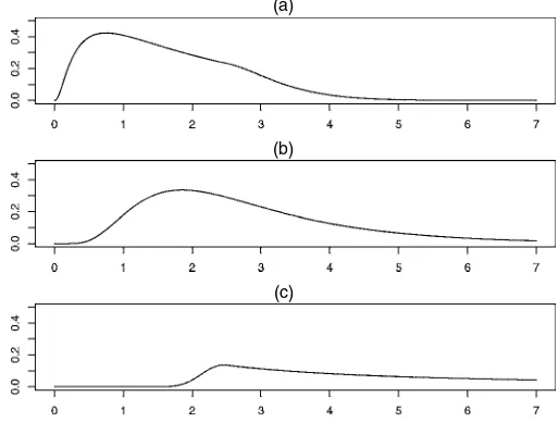
skew-ness and fat tails. By varying the parameters of the distributions in (4) and (5), we obtain a wide range of possible shapes for the implied distribution of WTP,wi=exp(yi)=exp(x′iβ+σ εi).
This is illustrated in Figure 1, which displays some typical
(a)
(b)
(c)
Figure 1. Sampling Densities of Positive WTP With the Skewed
Nor-mal Distribution in (4) for Various Values ofγ: (a)γ=.5; (b) γ=1;
(c)γ=4.
(a)
(b)
(c)
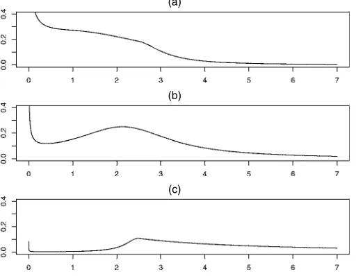
Figure 2. Sampling Densities of Positive WTP With the Skewed
Stu-dent Distribution in (5) forν=1 and Various Values ofγ: (a)γ=.5;
(b)γ=1; (c)γ=4.
shapes for the density function of WTP derived from (4) for various values ofγ, usingx′iβ=.92 andσ =.55, inspired by our empirical results (with WTP measured in thousands of pe-setas). Figure 2 gives some possible shapes for the pdf based on (5), where we have chosen the same values forγ ,x′iβ, and
σas in Figure 1, withν=1.
2.3 The Likelihood Function
In this section we derive the likelihood function obtained from the model in (1), with the specific choices made in (2)–(5). LetNbe the number of observations. We consider two possible survey formats:
1. Individuals that answer negatively to both bids, are also
asked whether their WTP=0. This is the case in our
practical application. Without loss of generality, we order the observations so that the first Npos≤Ncorrespond to
the individuals with positive WTP (in which case they are given as sets yi=log(wi)∈Si fori=1, . . . ,Npos). The
remaining observations correspond to WTP=0. Thus the
likelihood function is the model in (3) combined with either (4), in which case
ψ=γ, or (5), whenψ=(γ , ν). Note that this likelihood factorizes, with one factor involving onlyδand the other factor involving only(β, σ,ψ).
2. An alternative survey format, considered by, for example, Werner (1999), is when no further question is asked after the two bids. In that case, for individuals who respond negatively to both bids, we do not know whether their
WTP is zero or is positive but smaller than both bids of-fered, in which caseyi=log(wi)belongs to the implied
setSi. Assuming, without loss of generality, that the
in-dividuals that answered both times negatively are the last
N− ˜Nin the sample, the likelihood function now becomes
L(δ,β, σ,ψ)
because some of the people who answer negatively to both bids could have a strictly positive WTP. Our theoretical and compu-tational approach in this article can deal with both likelihoods, whereas our practical application relates to the first one.
2.4 The Prior Distribution
Because our inferential framework is Bayesian, we need to specify a prior distribution on the parametersδ,β,σ,γ, and, in case of model (5),ν. We choose a prior distribution that has a product structure for all parameters, as follows.
For δ, we adopt an m-variate normal g-prior (see Zellner 1986) given by
δ∼Nm0,N(Z′Z)−1, (8)
whereN is the total number of observations andZ≡(z1, . . . , zN)′ theN×mdesign matrix. Thisg-prior implies that prior
precision is a fraction 1/N of that of the sample and is often used in the context of vague prior information.
The regression coefficients inβ∈Rkand the scaleσ >0 are assigned the standard noninformative priors (see, e.g., DeGroot 1970, chap. 10), corresponding to the density
p(β, σ )∝ 1
σ. (9)
For known γ and ν, the prior in (9) is both Jeffreys’ prior under independence and the reference prior, as was shown by Fernández and Steel (1999a).
For the skewness parameter γ, we adopt a gamma prior
on γ2, where the hyperparameters are chosen to obtain
E(γ )=1, thus centering the prior forγ over the symmetric case while combining a reasonably large prior variance with a relatively balanced allocation of mass both sides of 1. This procedure leads to the following half-normal prior onγ:
γ∼N(0, π/2) truncated toγ >0. (10) In the case of (skewed) Student sampling, we take for the degrees of freedom parameter
ν∼exponential(mean=10), (11)
which captures a wide tail behavior.
We stress that, whereas the foregoing priors for δ, γ, and
νare our preferred choices in the absence of substantial prior in-formation, our analysis does not rely on these particular choices and would essentially carry over to any other proper priors for these parameters.
3. POSTERIOR DISTRIBUTION AND BAYES FACTORS
3.1 Propriety of the Posterior Distribution
In this section we deal with a technical but important issue. Our chosen prior distribution is improper—in other words, not integrable over the parameter range. As a consequence, propri-ety (i.e., integrability) of the posterior distribution, which un-derlies inference in a Bayesian framework, is not guaranteed and needs to be checked to make sure that Bayesian inference is possible with this prior choice. We remind the reader that propriety of the posterior is guaranteed if a proper prior distrib-ution is used, but we chose the improper prior in (9) because it is a convenient noninformative distribution.
First, we give a theorem that characterizes the propriety of the posterior distribution in a more general setting than the one in this article. We then build on this result to provide a second theorem that establishes a sufficient condition for propriety of the posterior distribution in our CV context.
Theorem 1. Lety1∈S1, . . . ,yM∈SM be independent
com-pact set observations from the model in (3) in combination with either (4) or (5). Consider the prior distribution
p(β, σ,ψ)∝ 1
σp(ψ),
wherep(ψ)is any probability distribution, (12)
withψ =γ under model (4) andψ=(γ , ν)under model (5).
Then, the posterior distribution is proper if and only if
rank(X:y)=k+1 for ally1∈S1, . . . ,yM∈SM, (13)
wherey=(y1, . . . ,yM)′andXis the correspondingM×k
ma-trix of explanatory variables.
Thus Theorem 1 provides a full characterization of propriety of the posterior distribution in the context of compact set obser-vations from a linear regression model where the error term is either normal, skewed normal, Student-t, or skewed Student-t, under the standard improper noninformative prior for the lo-cation and scale parameters. If in addition to compact sets, one has unbounded set observations, then the rank condition in The-orem 1 based only on the compact sets is sufficient for propriety of the posterior.
Theorem 2. Consider a double-bounded dichotomous choice CV survey withNindependent respondents, where the individ-uals who answer negatively to both bids may or may not be
asked whether their WTP=0. The assumed underlying model
for WTP is given by (1)–(3) combined with either (4) or (5). Consider the prior distribution
p(δ,β, σ,ψ)∝p(δ)1 σp(ψ),
wherep(δ)andp(ψ)are any probability distributions, (14)
withψ=γ under model (4) andψ=(γ , ν)under model (5).
Let yi=log(wi)∈Si,i=1, . . . ,M, be the (log-transformed)
set observations corresponding to individuals who answer pos-itively to one of the bids and negatively to the other one. Then if (13) holds for theseMset observations, the posterior distrib-ution is proper.
Our prior distribution in (8)–(11) is in the class described by (14). Thus Theorem 2 applies with the prior considered in this article.
To use Theorem 2, we need to have at leastk+1
individ-uals in the survey answer differently to both bids. Once this has been established, checking the rank condition (13) for the bounded setsS1, . . . ,SM can be nontrivial. For some problems,
the method outlined by Fernández and Steel (1999b, ex. 1) can simplify the task. In our application to the Teide National Park data, an even simpler way of checking can be used: We can find two compact set observations corresponding to the same covariates that do not overlap, which directly ensures that the rank condition holds.
Clearly, the more individuals who answer differently to both bids and the narrower the intervals observed, the better the chance that the rank condition in (13) holds. We stress, however, that this is merely a sufficient condition and that the posterior distribution could still be proper in cases where this condition fails.
3.2 Computation of the Posterior Distribution via Markov Chain Monte Carlo
Once the propriety of the posterior distribution is established, the latter must be computed via simulation. For this we use an MCMC algorithm, which, due to space restrictions, we sketch only briefly here.
We start by augmenting the data withN independent latent
variables,m1, . . . ,mN, wheremi has an N(z′iδ,1)distribution.
Thenwi>0 if and only ifmi>0.
When the likelihood is given by (6), we know from the ob-served data thatmi>0 fori=1, . . . ,Npos, andmi<0 for the
remaining observations. In addition, because of the factoriza-tion of this likelihood funcfactoriza-tion, inference onδand on(β, σ,ψ)
can be conducted separately. Forδ, we apply the standard Gibbs sampler for probit models, which updatesδand(m1, . . . ,mN)
by drawing them from their full conditional distributions in turns described in Fernández, Ley and Steel (2002). (see Al-bert and Chib 1993 for a similar analysis). The MCMC sampler for(β, σ,ψ)is based on an amalgamation of the sampler given by Fernández and Steel (1998), which deals with skewed Stu-dent sampling with point observations, and the idea of Fernán-dez and Steel (1999b) for handling set observations. For each
i=1, . . . ,Npos, we introduce a further latent variable,yi, with
distribution (3) combined with either of (4) or (5); when the model corresponds to (5), we augment further with a variable
λi which is gamma distributed with mean 1 and variance 2/ν.
(This handles the Student-tmodel by representing it as a scale mixture of normals.) Conditionally on the data and the values of all other parameters and augmented variables at the current state of the Markov chain, we drawβ, σ, γ,ν, (yi, λi) for
i=1, . . . ,Npos. In the case of (4), we do not sampleνorλi.
When the likelihood is given by (7), the MCMC sampler is different, because the previous likelihood factorization no longer applies. Note that now we do not know the sign ofmi
when i>N˜. In addition to mi, we augment with yi and λi
(as described in the previous paragraph) for all observations
i=1, . . . ,N. The MCMC algorithm then proceeds by sam-pling from the full conditional distributions ofδ, β, σ,γ,ν,
(mi,yi, λi)for i=1, . . . ,N. If the model corresponds to (4),
then we do not sampleνorλi.
3.3 Computing Bayes Factors for Model Comparison
The framework of Section 2 leads to four possible distribu-tional models for log(WTP). In particular, the distribution ofεi
in (3) can be normal [using (4) withγ =1], skewed normal
as in (4), Student-t[from (5) withγ=1], or skewed Student-t
as in (5). Within a Bayesian framework, formal model com-parison or model averaging can be conducted on the basis of Bayes factors (i.e., ratios of marginal likelihoods), which are well-defined as long as priors are proper on model-specific
pa-rameters. Because we have proper priors onγ andν, we can
compute Bayes factors for our four contending models. Poste-rior model probabilities are readily computed from pPoste-rior model probabilities and Bayes factors.
A convenient way to compute Bayes factors is by using the Savage–Dickey density ratio (see Verdinelli and Wasserman 1995). Consider a modelM1with, say, two parametersθandω
and a product structure prior, and a simpler modelM0, which is
the reduction ofM1asθtakes a fixed valueθ0. Then the Bayes
factor in favor ofM0 versusM1 will be equal to the ratio of
posterior and prior densities ofθunderM1atθ=θ0.
In our context, comparing a symmetric model and its skewed counterpart thus can be immediately implemented by compar-ing prior and posterior densities ofγ under the skewed model evaluated atγ=1.
Comparing Student and normal tails is less immediate. If we focused on the degrees of freedom parameterν(as in Verdinelli and Wasserman 1995), then we would have to consider the lim-iting caseν= ∞for normality, which is, strictly speaking, not a value in the domain ofνand, hence the foregoing ratio would not apply. In addition, most priors would lead to a 0/0 den-sity ratio asν→ ∞. However, if we consider the representa-tion of the Student-tdistribution as a scale mixture of normals (as mentioned in Sec. 3.2), then the normal distribution does
be-come a special case, where the mixing parameterλ=1. Thus
we can compute the Bayes factor from the prior and posterior densities of(λ1, . . . , λQ)under the fat-tailed model evaluated
at(λ1, . . . , λQ)=(1, . . . ,1), whereQ=Nposfor likelihood (6)
andQ=Nfor likelihood (7). Note that this method directly ex-tends to comparing normal models with any scale mixture of normals, not just Student models.
4. PREDICTING WILLINGNESS TO PAY AND PRICE–SETTING
4.1 The Predictive Distribution of Willingness to Pay
Because one of the main quantities of interest is WTP, we focus on inference on WTP rather than on model parameters.
Given the regression context in (2) and (3), the predictive distri-bution of WTP (i.e., the conditional distridistri-bution of WTP given only the observed data),wf, depends on individual
character-istics grouped in covariate vectorszf andxf. In practice,
how-ever, we often will be interested not in predicting the WTP of an individual with a particular set of characteristics, but rather in inference on WTP for an individual randomly drawn from the target population. This implies that we need to mix over pos-sible values for the individual characteristics, and, given that we have no further information on their distribution in the pop-ulation, we use the empirical distribution of characteristics in the observed sample; that is, we assign weight 1/Nto each of
(z1,x1), . . . , (zN,xN). Given the size of the sample in our
appli-cation (N=941), this seems not too crude an assumption. This mixed predictive distribution for WTP, saywmix, is given by
1. wmix=0 (15)
with probability 1−prmix≡1−N1N
i=1pri,where
pri≡ (z′iδ)p(δ|data)dδ. (16)
This integral can be calculated by averaging (z′iδ)over the
posterior draws ofδgenerated through the MCMC sampler.
2. With probabilityprmix,wmix>0, and it has pdf
exp(yi) corresponding to (3) in combination with either
(4) or (5). This integral can also be easily evaluated by aver-aging the density functionpwi(w|β, σ,ψ,xi)over the posterior draws of(β, σ,ψ). We also can average the predictive distrib-ution of WTP over distribdistrib-utional models with the appropriate posterior model probabilities (computed from the Bayes fac-tors; see Sec. 3.3). Thus we have a formal framework for deal-ing with both parameter and distributional uncertainty.
4.2 The Predictive Distribution of Revenue and Price-Setting
In the context of Teide National Park, a particularly interest-ing use of the WTP distribution is to determine what fraction of potential visitors would be expected to enter the park at a given price. This can then be straightforwardly used to determine ex-pected revenue (per potential visitor) at a certain price, by sim-ply multisim-plying the latter fraction with the entry price. For a price A, this naturally leads to a focus on P(wmix≥A|data),
and from (15)–(17) this is equal to
N
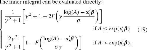
The inner integral can be evaluated directly:
skewed normal sampling) or the Student-t withν degrees of
freedom (for skewed Student sampling). Hence the probability in (18) can be computed simply by averaging the values of the expression in square brackets with respect to the MCMC poste-rior draws.
As indicated earlier, we can predict expected revenue (per potential visitor) with an entry priceAby multiplying the prob-ability in (18) byA. The behavior of expected revenue as a func-tion of the priceAcan be most useful in establishing an entry fee to the park. One might be interested in finding the price that maximizes expected revenue. The existence of such a revenue-maximizing price is not guaranteed in general, however. For example, we can show that under skewed Student sampling, expected revenue given any parameter values (i.e., in the sam-pling) tends to infinity asA→ ∞. The expected revenue (again given parameter values) for the skewed normal case appears
to be better behaved, because it goes to 0 as A→ ∞and
al-ways has a finite global maximum. Empirical predictive results for our particular application seem to reproduce this behavior. Of course, maximizing revenue may not be the only considera-tion when setting a price, because the proporconsidera-tion of people that actually enter the park (and thus benefit from the natural re-source) can also be of interest. In particular, we would want to avoid a situation where we set the price so high that only very few people are willing to pay the entry fee, even if the expected revenue for that price is large.
Generally, if we are interested in finding the priceAat which a proportionpof the target population can be expected to enter the park, then we simply note thatE[Revenue(A)] =Ap, so that we can find the appropriateAas thex-coordinate of the inter-section point of expected revenue (plotted as a function ofA) and a straight line through the origin with slopep. This is il-lustrated in Figure 5 (see Sec. 6.2), where several values ofp, ranging from .75 to .01 are considered. Thus, for example, take the intersection of expected revenue with the line corresponding top=.25; thex-coordinate tells us that at a price of 2,130 pese-tas (Ppese-tas), 25% of the potential visitors are expected to enter the park, thus leading to an expected revenue per potential visitor of 532.5 Ptas (on they-coordinate). (At the time of the survey, 1 U.S. dollar was equivalent to about 157 Spanish pesetas.)
Of course, Revenue(A)is a random variable, and its expecta-tion is merely one property of its distribuexpecta-tion. For any potential visitor and entry feeA, Revenue(A)has a discrete two-point dis-tribution with probabilityP(WTP<A)at Revenue(A)=0 and probabilityP(WTP≥A)at Revenue(A)=A. Thus its variance is equal toA2P(WTP<A)P(WTP≥A), so that both the mean and the variance of Revenue(A)depend on the entry feeA. The distribution of total revenue over a large number of potential visitors is close to normal, due to the central limit theorem. Figure 6 shows the predictive distribution of total revenue over
3 million potential visitors for two different entry prices; we discuss these figures further in Section 6.
Examining the predictive distribution of revenue may not be the most traditional form of public good pricing, but it fits in very well with the increasing importance of ecotourism as a sustainable use of protected natural areas, especially in devel-oping countries. Chase, Lee, Schulze, and Anderson (1998) and Walpole, Goodwin, and Ward (2001) have examined pricing policies for national parks in Costa Rica and Indonesia.
CV studies in the literature often report summary measures of WTP, such as the mean or median. We stress that one should carefully distinguish between these commonly used summary measures of WTP and expected revenue if one such measure is set as the entry price. Trivially from the definition of revenue, if the entry price is set to be equal to median WTP, then ex-pected revenue will be only half that amount. In addition, the following proposition shows that expected revenue is always smaller than mean WTP.
Proposition 2. For any entry priceA and regardless of the distribution of WTP, we have
E[Revenue(A)]<E(WTP).
E(WTP)has the convenient property that it is preserved un-der aggregation. This means that expected total WTP for a pop-ulation can be obtained simply by adding the expected WTP of each individual in the population. (Note that this aggregation property does not hold for median WTP.) Such an expected to-tal WTP may well be an important welfare instrument if we consider introducing certain programs (e.g., a set of regulations to reduce pollution, a land acquisition program) and there is a possibility for individuals with high WTP to compensate those with low (or even negative) WTP. This is clearly a much less relevant concept in our pricing context, where every individ-ual pays the same entry fee. The relevant quantity for us is the proportion of people in the population that are willing to pay a certain price, and, accordingly, we need to focus on the proba-bility that WTP (aswmix) is above any given price.
5. THE TEIDE NATIONAL PARK DATA
It this survey, conducted in the summer of 1997, subjects were interviewed in Mount Teide National Park on Tenerife, in the Canary Islands archipelago. At 3,718 meters (12,198 ft.), the volcano Teide is the highest peak in Spanish territory. The park is home to a large expanse of so-called “supracanario” veg-etation and offers visitors one of the most spectacular examples of a volcanic landscape in the world.
The subjects were approached as they were about to leave the park, to ensure that they had already experienced the visit. At the time of the interviews, entrance to the park was free. People were asked their valuation of the park in terms of how much they would be willing to pay to enter. They were told that these (hypothetical) fees would be used to maintain the natural beauty of the park. As explained in Section 2.1, indi-viduals were presented with two successive bids. Those who responded negatively to both questions were also asked whether their WTP=0 and, if so, to state the reason for this. Thus the likelihood is given by (6). From the survey, we obtainN=941
Figure 3. The Data Information and Skewed Normal Predictive Den-sities for WTP. The interval data corresponding to the nonzero re-sponses is given by the solid line, and at zero there is a point mass of .187. The other lines represent predictive distributions on WTP, which has a point mass at zero while the remaining mass is
allo-cated to a density function for positive WTP ( data; mixed;
minimum; mode; maximum). The four predictives
corre-spond to different values of the covariates, and are all derived under the skewed normal sampling model for positive WTP.
valid responses, of whichNpos=765 are positive, in the form
of set observations. Note that 18.7% of all interviewed individ-uals stated that they were not willing to pay anything to enter the park. For the others, we obtainM=359 compact sets for log(WTP), corresponding to people who replied “yes” to one offered price and “no” to another. All questions were asked in terms of the individual’s national currency and then converted to Ptas.
A graphical display of the positive WTP responses is pro-vided in Figure 3 (as “data”), where the total mass assigned to the set observations (81.3%) is uniformly distributed over all
Npos=765 observations. Thus the figure displays a mixture of
uniform density functions on each set observation with weights equal to.813/765. In addition, the empirical mass at 0 is .187. In terms of WTP, sets can be unbounded only on the right, and whenever this occurs, we truncate (only for the purpose of this graphical presentation) at 10,000 Ptas.
In addition to questions about the WTP, the survey also records some individual characteristics. In accordance with economic theory and the empirical CV literature, we choose the following covariates:
• BEFORE, a dummy (i.e., 0–1) variable indicating whether
or not the subject has visited the park before. The variable takes the value 1 if there was a previous visit.
• INFO, a dummy variable indicating whether or not the
subject had previous information regarding the park. The value 1 corresponds to previous information.
• EDU, the number of years of formal education.
• AGE, age in years.
• IMP, a dummy variable indicating whether or not the
ex-istence of the park was an important reason for visiting Tenerife. IMP=1 denotes that the park was important.
• INC, monthly personal income (expressed in Ptas).
• NAT, a categorical variable indicating nationality
(TF, Tenerife; SP, rest of Spain; GER, Germany; UK, United Kingdom; IT, Italy; FR, France; NL, Netherlands; rest, all other countries).
We use these variables to construct appropriate covariate vec-tors zi for the probit part of the model in (2) and xi for the
regression part of the model in (3). Generally, we based the choice of which variables to include on both posterior and pre-dictive results [note that the improper prior on β in (9) does not allow for formal posterior odds], and we typically trans-formed continuous covariates to logarithms. We also experi-mented with transforming continuous variables into categorical variables (which can capture nonlinear effects). We excluded a covariate if the posterior distribution of its regression coeffi-cient assigned roughly the same amount of mass to both sides of 0, if we could not find a suitable transformation for which this was not the case, and if excluding it did not adversely af-fect the (within-sample) predictive performance of the model.
6. EMPIRICAL RESULTS
6.1 Posterior Findings and Bayes Factors
We first present some posterior results, based on running the sampler briefly described in Section 3.2 for a burn-in period of 10,000 draws and then retaining every 10th draw of the next 120,000 draws. Convergence checks do not indicate any prob-lems. Extensive experimentation leads to the specification for which we present posterior results in Table 1. The results for the positive part of WTP are based on the skewed normal specifica-tion, which turns out to be the model most favored by the data
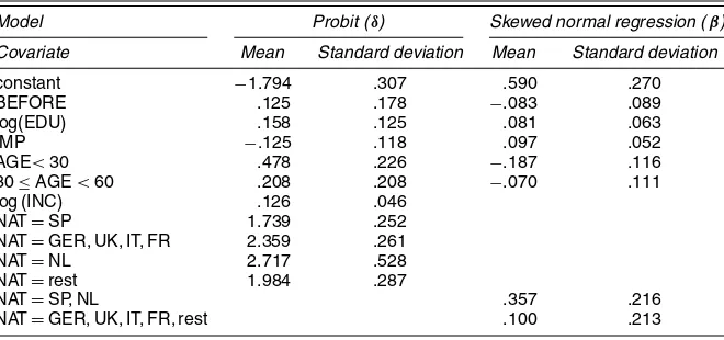
Table 1. Posterior Moments of the Regression Coefficients
Model Probit (δ) Skewed normal regression (β)
Covariate Mean Standard deviation Mean Standard deviation
constant −1.794 .307 .590 .270 BEFORE .125 .178 −.083 .089 log(EDU) .158 .125 .081 .063 IMP −.125 .118 .097 .052 AGE<30 .478 .226 −.187 .116 30≤AGE<60 .208 .208 −.070 .111 log (INC) .126 .046
NAT=SP 1.739 .252 NAT=GER, UK, IT, FR 2.359 .261 NAT=NL 2.717 .528 NAT=rest 1.984 .287
NAT=SP, NL .357 .216 NAT=GER, UK, IT, FR, rest .100 .213
(a) (b)
(c) (d)
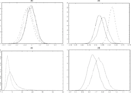
Figure 4. Posterior Densities of Model Parameters for Positive WTP Under the Different Sampling Models: (a) log(EDU); (b) σ; (c) ν;
(d)γ. ( normal; Student; skewed normal; skewed Student.)
(see later). The moments ofβreported in Table 1 can be shown to exist using arguments similar to the proof of Theorem 2 (they trivially exist forδ). Note thatziandxihave some overlap, but
are not the same. In particular, the grouping of nationality dif-fers between the zero and positive WTP parts of the model; Tenerife is the reference category for both parts. With respect to this reference category, we see that, for example, visitors from the Netherlands tend to have higher probabilities of pos-itive WTP and higher values of the pospos-itive WTP. Income has a pronounced effect on the probability of positive WTP (which tends to increase with income), but no discernible effect on the amount of WTP once it is positive. The reference category for
AGE is the class AGE≥60, and this category has the lowest
probability of positive WTP; however, if WTP is positive, then the older age categories tend to have higher WTP. A referee suggested that this might be due to the effect of wealth, which is not captured in our available information set. Most older peo-ple have limited incomes, but some have accumulated wealth. Hence, when older people have a positive WTP, they may have a higher WTP than younger individuals who have yet to accumu-late much wealth. Most of them=11 andk=8 regression co-efficients have posterior means that are not counterintuitive. For example, higher levels of education are associated with higher probability of positive WTP and higher values of WTP if posi-tive.
The posterior density function of the latter coefficient is plot-ted in Figure 4(a) for all four possible regression models for positive set observations. The effect of log(EDU) on the loca-tion of log(WTP) is somewhat larger for the skewed models, but differences between the specifications are not huge. Fig-ures 4(b)–(d) display the posterior densities ofσ andνfor the Student models andγ for the skewed models. Generally, there is some evidence of fat tails and left skewness in the log(WTP) distribution. However, if both skewness and fat tails are in-cluded simultaneously, then the latter evidence seems less pro-nounced.
Bayes factors between the four distributional specifications considered here for the positive observations were computed as indicated in Section 3.3. The results, given in Table 2, are clearly in favor of the skewed normal model. (Note that the en-tries in the table are the log Bayes factors of the models in the
Table 2. Log Bayes Factors Between Contending Regression Models
Skewed Student Student Skewed normal Normal
Skewed Student 1 2.2 −231 42.2 Student 1 −233.2 40 Skewed normal 1 273.2
Normal 1
NOTE: The entries are the logarithms of the Bayes factor of the model in the row versus the model in the column.
row versus the model in the column.) In order of preference, the data favor the skewed normal, the skewed Student, the Stu-dent, and the normal distributions. In particular, the support for the skewed normal model is overwhelming. Therefore, mixing over models is not critical, because the averaged predictive sults would be indistinguishable from the skewed normal re-sults, and we shall present results only for that specification in the sequel.
6.2 Predictive Results
For the probit part of the model, we compute the probability of positive WTP, as in (16), for covariate combinationszi
corre-sponding to each observationi=1, . . . ,Nin the sample. Thus we obtain a set ofN predictive probabilities of positive WTP, which range from .043 to .977 and lead to an average over all observations ofprmix=.812, very close to the sample
propor-tion of positives. The wide range indicates that the regressors inzf really matter for the probability of zero WTP. To
evalu-ate whether the regressors actually help in correctly predicting zero versus positive WTP, we compute the average probabil-ity of zero for those N−Npos=176 observations that were
actually recorded as zeros: this average is .441. The average predictive probability of zero WTP for theNpos=765 positive
observations is .130. This suggests that our model provides a reasonable fit to the data (at least substantially better than with a constant probability of zero WTP).
Taking the probit and the regression parts of the model into account, as in Section 4.1, we first focus on predictingwf given
three sets of regressor values,(zf,xf). These are chosen as
fol-lows. First,(zmod,xmod)are based on the modal values of each covariate in the sample. Taking means instead would not lead to observable values for categorical regressors, and in the pres-ence of unordered categorical variables, medians make little sense. The vectorxminis chosen as the set of within-sample
val-ues for the regressors that minimizesx′βat the posterior mean forβ. (Thus, e.g., for elements in β with positive mean, we take the smallest observed value of the corresponding regres-sor.) Similarly, we choosexmax. Of course, this does not yet
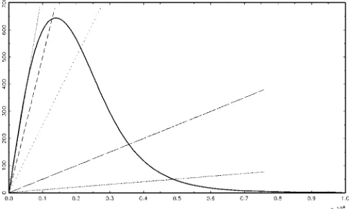
Figure 5. Expected Revenue per Potential Visitor as a Function of Entrance Price for the Skewed Normal Model and Mixed Over the Re-gressors With the Observed Distribution. The straight lines with slopes
p<.812 intersect with the expected revenue curve at the price where
a fraction p of the target population is expected to enter the park.
( revenue; p=.75; p=.50; p=.25; p=.05;
p=.01.)
Table 3. Entry Prices and Expected Revenue for Fractions Entering (skewed normal)
Fraction entering (p) .75 .50 .25 .05 .01 .001
Entry price (Ptas) 540 1,280 2,130 3,550 4,900 7,000 Expected revenue 405 640 532.5 177.5 49 7
definezmin andzmax, which also require a value for log(INC)
and have a finer partition of nationalities (see Table 1). We
chose zmin and zmax using the modal income and the modal
country within each group of countries used for positive WTP. The predicted probabilities of positive WTP are quite differ-ent for these three covariate combinations: prmin=.235 (for zmin),prmod=.917, andprmax=.688. Figure 3 displays how
these probabilities are distributed over positive WTP. There is a clear difference in location for the three vectorsxf. Although
the combination (xmod,zmod)is closest to the empirical data distribution in location, it overestimates the overall probability of positive WTP. If, instead, we mix over all observed regressor combinations, as explained in Section 4.1, then we obtain the predictive density function indicated by “mixed” in Figure 3 (whereprmix=.812 as indicated earlier). Clearly, this fits the
empirical data distribution reasonably well.
As already stressed in Section 4.2, the expected revenue per potential visitor is of particular interest to us. Figure 5 presents predictive expected revenue (mixed over the regressors with the empirical distribution) as a function of entry price for the skewed normal regression model specification. Intersections of the expected revenue curve and the straight lines with slopes
pdefine the prices at which a fractionpof the target population is expected to enter the park. Table 3 provides more numerical detail on the particular values for price and expected revenue corresponding to various values of p. As we know, a certain fraction of people are not willing to pay any positive price at all for entry. Thus we can find positive prices only for which the proportionp of people entering is less thanprmix=.812.
The entry price that maximizes expected revenue is 1,380 Ptas, leading to an expected revenue of 644 Ptas per potential visi-tor. Thus the expected fraction of potential visitors willing to pay this amount isp=.467, and we would be charging slightly more than the median WTP as entry fee.
Figure 6 shows the predictive distribution of total revenue (in millions of Ptas) obtained from a typical annual amount of
(a) (b)
Figure 6. The Predictive Distribution of Total Revenue (in millions of Ptas) Obtained From 3 Million Visitors (the average annual number) to Mount Teide National Park. (a) The revenue distribution for an entry price of 1,380 Ptas, the one that maximizes expected revenue. (b) The rev-enue distribution for an entry price of 540 Ptas, so that only 25% of the potential visitors will choose not to pay.
visitors (3 million). Figure 6(a) shows revenue for an entry fee of 1,380 Ptas, which we know maximizes expected revenue. Figure 6(b) considers an entry fee of 540 Ptas, which corre-sponds to only 25% of potential visitors choosing not to enter (as shown in Table 3). Note that total revenue is very precisely predicted on the basis of our analysis.
7. CONCLUDING REMARKS
The development of Bayesian methods enhances the statis-tical toolbox with which inference on CV data can be con-ducted. Bayesian methods allow the analyst to incorporate prior information if available (although in this article we have used noninformative priors instead), and naturally lead to predictive inference while providing a straightforward approach to deal-ing with model uncertainty. In this article we have shown how Bayesian inference can be conducted for interval data on WTP as obtained from a double-bounded dichotomous choice survey. Application of our methodology to the one-and-one-half-bound approach of Cooper et al. (2002) is immediate. In principle, our inference methods could also be adapted to settings where some dependence of WTP on the bids is allowed for.
Our model explicitly incorporates zero responses on WTP by means of a probit model, which is combined with flexible distri-butional assumptions on positive WTP (observed as intervals). Inference is conducted conditionally on the observed intervals. Bayes factors are used to compare the competing valuation distribution assumptions. In our application, the skewed normal distribution for log(WTP) is favored over normal, Student, and skewed Student models.
The predictive distribution leads to an expected revenue func-tion that can be useful for pricing decisions on the access to public goods, especially in the context of the increasing im-portance of ecotourism in developing countries. The empirical analysis with data from the Teide National Park in Spain shows that expected revenue is maximized by setting an entry price of 1,380 Ptas, which is slightly higher than the median WTP. Although not implemented here, differential pricing policies (e.g., charging different fees to the local and foreign popula-tions) can be immediately accommodated by our framework.
The framework discussed in this article can easily be ap-plied in various other related contexts in which bounded and unbounded interval data are present, such as models for dose-response, reliability, and life testing.
ACKNOWLEDGMENTS
We gratefully acknowledge constructive comments from two referees, the associate editor, and Frédéric Jouneau. Fernández and Steel benefitted from a travel grant awarded by the Spanish Ministerio de Educación, Cultura y Deportes, Dirección Gen-eral de Universidades, and acknowledge the hospitality of the University of Las Palmas de Gran Canaria.
APPENDIX: PROOFS
Proof of Proposition 1
For each individual, our data are (B1,A1,B2,A2), where
B1andB2denote the values of the bids offered andA1andA2
denote the individual’s (yes/no) responses to each of the bids. From assumptions (a) and (b) and the assumption that individu-als answer in accordance with their WTP, the joint distribution factorizes as
tribution of WTP given the observed data is
p(WTP|B1,A1,B2,A2)∝p(WTP),
with WTP restricted toS(B1,A1,B2,A2),
whereS(B1,A1,B2,A2)is the set for WTP implied by the
an-swers to the bids offered.
Proof of Theorem 1
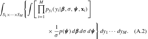
The posterior distribution is proper if and only if the denom-inator in Bayes’ theorem, from (3) in combination with (4) or (5). We can use Fubini’s theorem to reverse the order of integration and thus express the latter integral as
An argument parallel to the proof of theorem 1 of Fernández and Steel (1998) shows that the inner integral in (A.2) has up-per and lower bounds that are both proportional to the value of that same integral whenγ =1. Thus, as far as propriety of the
posterior is concerned, we can assume thatγ=1 (symmetric
case). This allows us to use theorem 3 of Fernández and Steel (1999b) to establish the rank condition in our Theorem 1.
Proof of Theorem 2
The model in Theorem 2 corresponds to the likelihood func-tion in either (6) or (7). In both cases, each of theN factors in the likelihood is less than or equal to 1, so the likelihood func-tion is bounded above by
M
i=1 Si
pyi(yi|β, σ,ψ,xi)dyi, (A.3)
wherei=1, . . . ,M are the indexes corresponding to individ-uals that answered differently to both bids. Thus, integrability
of the expression in (A.3) with respect to the prior distribution of(δ,β, σ,ψ)will imply a proper posterior. Integrating outδ
is trivial, becausep(δ)in (14) is proper. A necessary and suffi-cient condition for integrating out(β, σ,ψ)is provided by The-orem 1.
Proof of Proposition 2
Denoting bypWTP(·)any pdf for WTP, we have
E[Revenue(A)] =AP(WTP≥A)
=
∞
A
ApWTP(w)dw
<
∞
A
wpWTP(w)dw+
A
0
wpWTP(w)dw
=E[WTP]. (A.4)
[Received December 2002. Revised January 2004.]
REFERENCES
Alberini, A. (1995), “Efficiency vs. Bias of Willingness-to-Pay Estimates: Bi-variate and Interval-Data Models,”Journal of Environmental Economics and Management, 29, 169–180.
Albert, J. H., and Chib, S. (1993), “Bayesian Analysis of Binary and Polychoto-mous Response Data,”Journal of the American Statistical Association, 88, 669–679.
Blumenschein, K., Johannesson, M., Yokoyama, K. K., and Freeman, P. R. (2001), “Hypothetical versus Real Willingness to Pay in the Health Care Sector: Results From a Field Experiment,”Journal of Health Economics, 20, 441–457.
Buckland, S. T., Macmillan, D. C., Duff, E. I., and Hanley, N. (1999), “Esti-mating Willingness to Pay From Dichotomous Choice Contingent Valuation Studies,”The Statistician, 48, 109–124.
Cameron, T. A., and Huppert, D. D. (1991), “Referendum Contingent Valuation Estimates: Sensitivity to the Assignment of Offered Values,”Journal of the American Statistical Association, 86, 910–918.
Carson, R. T., Flores, N. E., and Meade, N. F. (2001), “Contingent Valuation: Controversies and Evidence,”Environmental and Resource Economics, 19, 173–210.
Chase, L. C., Lee, D. R., Schulze, W. D., and Anderson, D. J. (1998), “Eco-tourism Demand and Differential Pricing of National Park Access in Costa Rica,”Land Economics, 74, 466–482.
Cooper, J. C., Hanemann, W. M., and Signorello, G. (2002), “One-and-One-Half-Bound Dichotomous Choice Contingent Valuation,” Review of Eco-nomics and Statistics, 84, 742–750.
DeGroot, M. H. (1970),Optimal Statistical Decisions, New York: McGraw-Hill.
Fernández, C., and Steel, M. F. J. (1998), “On Bayesian Modeling of Fat Tails and Skewness,”Journal of the American Statistical Association, 93, 359–371.
(1999a), “Reference Priors for the General Location-Scale Model,”
Statistics and Probability Letters, 43, 377–384.
(1999b), “Multivariate Student-tRegression Models: Pitfalls and In-ference,”Biometrika, 86, 153–167.
Hanemann, M., and Kanninen, B. (1999), “Statistical Analysis of Discrete Choice Response CV Data,” inValuing Environmental Preferences, eds. I. J. Bateman and K. G. Willis, Oxford, U.K.: Oxford University Press, pp. 302–441.
Hanemann, W. M., Loomis, J., and Kanninen, B. (1991), “Statistical Efficiency of Double-Bounded Dichotomous Choice Contingent Valuation,”American Journal of Agricultural Economics, 73, 1255–1263.
Heitjan, D. F., and Rubin, D. B. (1991), “Ignorability and Coarse Data,”The Annals of Statistics, 19, 2244–2253.
Herriges, J. A., and Shogren, J. F. (1996), “Starting Point Bias in Dichotomous Choice Valuation With Follow-up Questioning,”Journal of Environmental Economics and Management, 30, 112–131.
Kriström, B. (1997), “Spike Models in Contingent Valuation,”American Jour-nal of Agricultural Economics, 79, 1013–1023.
Loomis, J., Traynor, K., and Brown, T. (1999), “Trichotomous Choice: A Pos-sible Solution to Dual-Response Objectives in Dichotomous-Choice Contin-gent Valuation Questions,”Journal of Agricultural and Resource Economics, 24, 572–583.
Mitchell, R. C., and Carson, R. T. (1989),Using Surveys to Value Public Goods: The Contingent Valuation Method, Washington, DC: Resources for the Fu-ture.
Reiser, B., and Shechter, M. (1999), “Incorporating Zero Values in the Eco-nomic Valuation of Environmental Program Benefits,”Environmetrics, 10, 87–101.
Verdinelli, I., and Wasserman, L. (1995), “Computing Bayes Factors Using a Generalization of the Savage–Dickey Density Ratio,”Journal of the Ameri-can Statistical Association, 90, 614–618.
Walpole, M. J., Goodwin, H. J., and Ward, K. G. R. (2001), “Pricing Policy for Tourism in Protected Areas: Lessons From Komodo National Park, Indone-sia,”Conservation Biology, 15, 218–227.
Werner, M. (1999), “Allowing for Zeros in Dichotomous-Choice Contingent-Valuation Models,”Journal of Business & Economic Statistics, 17, 479–486. Zellner, A. (1986), “On Assessing Prior Distributions and Bayesian Regres-sion Analysis With g-Prior Distributions,” inBayesian Inference and Deci-sion Techniques: Essays in Honor of Bruno de Finetti, eds. P. K. Goel and A. Zellner, Amsterdam: North-Holland, pp. 233–243.