Full Terms & Conditions of access and use can be found at
http://www.tandfonline.com/action/journalInformation?journalCode=ubes20
Download by: [Universitas Maritim Raja Ali Haji] Date: 12 January 2016, At: 17:56
Journal of Business & Economic Statistics
ISSN: 0735-0015 (Print) 1537-2707 (Online) Journal homepage: http://www.tandfonline.com/loi/ubes20
The Sensitivity of Productivity Estimates
Johannes Van Biesebroeck
To cite this article: Johannes Van Biesebroeck (2008) The Sensitivity of Productivity Estimates, Journal of Business & Economic Statistics, 26:3, 311-328, DOI: 10.1198/073500107000000089 To link to this article: http://dx.doi.org/10.1198/073500107000000089
Published online: 01 Jan 2012.
Submit your article to this journal
Article views: 213
View related articles
The Sensitivity of Productivity Estimates:
Revisiting Three Important Debates
Johannes V
ANB
IESEBROECKDepartment of Economics, University of Toronto, Toronto, Ontario, M5S 3G7, Canada (johannes.vanbiesebroeck@utoronto.ca)
Researchers interested in estimating productivity can choose from an array of methodologies, each with its strengths and weaknesses. This study compares productivity estimates and evaluates the extent to which the conclusions of three important productivity debates in the economic development literature are sensi-tive to the choice of estimation method. Five widely used techniques are considered, two nonparametric and three parametric: index numbers, data envelopment analysis, instrumental variables estimation, sto-chastic frontiers, and semiparametric estimation. Using data on manufacturing firms in two developing countries, Colombia and Zimbabwe, we find that the different methods produce surprisingly similar pro-ductivity estimates when the measures are compared directly, even though the estimated input elasticities vary widely. Furthermore, the methods reach the same conclusions on two of the debates, supporting en-dogenous growth effects and showing that firm-level productivity changes are an important contributor to aggregate productivity growth. On the third debate, only with the parametric productivity measures is there evidence of learning by exporting.
KEY WORDS: Endogenous growth; Input reallocation; Learning by exporting; Within-firm growth.
1. MOTIVATION
Productivity measurement has become ever more widespread since Solow’s first decomposition of output growth into the contribution of input growth and a residual productivity term. Productivity is often used as a performance benchmark to rank firms or countries or to measure the rate of performance im-provement over time; for example, in industrial economics, a large literature investigates the effect of research and develop-ment (R&D) on productivity and the resulting impact on indus-try structure (Griliches 1994). In international economics, the impact of trade liberalization is now as likely to be measured by firm-level productivity changes as by changes in price-cost margins (Tybout and Westbrook 1995). Such rankings gained credibility once studies documented that productivity is posi-tively correlated with other indicators of success, such as profit, employment growth, export status, technology adoption, and mere survival. But the same time, the concept is not without am-biguity. Many different ways of measuring productivity exist, each relying on some untestable assumptions. Consequently, the reader is often left in some doubt as to how sensitive the conclusions of a given study are to the particular productivity measure used.
Given the objective of productivity measurement to identify output differences that cannot be explained by input differences, at least six issues will affect how successful various method-ologies are at accomplishing this. First, it must be specified whether or not all firms share the same production technology and input trade-off. Second, most methods require a functional form assumption, or at least some restrictions, on the deter-ministic portion of the production technology. Third, especially when some heterogeneity in technology is allowed, an assump-tion on firm behavior is needed to learn about the technological differences. Fourth, when technology is assumed to be homo-geneous across firms, it can be estimated econometrically, but the well-known problem of endogeneity of input choices must be controlled for. Fifth, to distinguish productivity from other unobservable elements that affect output, some structure must
be placed on the stochastic evolution of the unobserved pro-ductivity difference. Sixth, methodologies differ in sensitivity to measurement error in output or inputs; this is likely to be important especially in less intensively used datasets from de-veloping countries.
This study evaluates five widely used methodologies that deal with the foregoing issues differently. Index numbers are relatively flexible in the specification of technology but do not allow for measurement error. Assuming that firms minimize costs and that goods markets are competitive, index numbers provide an exact measure of productivity without the need to estimate the full range of input substitution possibilities. Data envelopment analysis is an entirely nonparametric method. Pro-duction plans are explicitly compared with the frontier, which is constructed as a linear combination of “efficient” production plans in the sample. The method is deterministic, but the bench-mark is intuitive from an activities analysis standpoint.
The three parametric methods that we consider calculate pro-ductivity from an estimated production function. Because the framework is explicitly stochastic, it is less vulnerable to mea-surement error, especially in output, but misspecification of the production function can be an issue. Estimators differ most importantly in how they control for the simultaneity of pro-ductivity and input choices. The system generalized method-of-moments (GMM) estimator (see Blundell and Bond 1998) relies on exogeneity assumptions on lagged inputs and output to generate instruments; productivity is assumed to follow an AR(1) process with a firm-specific intercept. Stochastic frontier estimators make distributional assumptions on the unobserved productivity differences to construct a likelihood function for the observed variables; the evolution of productivity must be modeled explicitly. The semiparametric approach, pioneered by
© 2008 American Statistical Association Journal of Business & Economic Statistics July 2008, Vol. 26, No. 3 DOI 10.1198/073500107000000089
311
Olley and Pakes (1996), exploits the information on ity differences contained in the investment decision; productiv-ity is assumed to follow a Markov process.
To evaluate the sensitivity of the results to the five mea-surement methodologies, we first compare the estimates di-rectly. The parametric methods produce point estimates and standard errors for the production function parameters, which can be compared with the entire distribution of input elastic-ities (weights) that the nonparametric methods calculate. For the productivity-level and growth estimates, we discuss the cor-relations between the various measures, as well as a number of summary statistics for the productivity distributions.
Second, we verify whether the conclusions from important debates in the productivity literature depend on the productiv-ity measure used. We focus on three questions, which have re-ceived much attention in development economics:
• Can the often-observed positive correlation between pro-ductivity level and export status be explained entirely by self-selection of more productive firms (plants) into the export market, or is there a role for learning-by-exporting effects?
• Which variables, if any, are consistently associated with productivity growth resulting from knowledge acquisition, as modeled in the endogenous growth literature?
• How important is firm-plant-level productivity change rel-ative to the reallocation of output between production units as a source of aggregate productivity growth for the indus-try?
Each question concerns a different aspect of the productiv-ity distribution. The first question compares productivproductiv-ity levels across firms, the second compares growth rates, and the third depends on changes in the entire productivity distribution. To-gether, they allow a comprehensive overview of the impact of measurement methodology. In earlier work (Van Biesebroeck 2006), we took a different approach, comparing the robustness of different methodologies using Monte Carlo simulations.
Two data sources are used to evaluate the robustness of the different methods, one containing the universe of textile plants in Colombia from 1977 to 1991 and the other a sample of man-ufacturing firms from Zimbabwe from 1993 to 1995. The two datasets provide distinct case studies. The Zimbabwean firms operate in a low-income country with a relatively small and underdeveloped manufacturing sector. Firms produce a variety of products, possibly using different technologies. The Colom-bian plants operate in a medium-income country that is ap-proximately three times as large and has a longer history of manufacturing. The plants are all in the textile industry, which is relatively open to international competition, and are likely to operate with a production technology that is more homoge-neous.
Both datasets (or similar ones in the respective regions) have been used extensively, not least to study the three questions that we focus on here. There is little consensus in the literature. The learning-by-exporting question has been studied for Colombia by Isgut (2001) and Clerides, Lach, and Tybout (1998). The for-mer highlighted the positive correlation between exporting and productivity, whereas the latter found that the correlation can be explained entirely by self-selection. In contrast, we (Van Biese-broeck 2005a) found robust learning-by-exporting effects for
Zimbabwe and other sub-Saharan African countries. In terms of the second debate, several studies have stressed that technol-ogy created in developed countries is likely to be inappropri-ate for developing countries (see, e.g., Acemoglu and Ziliboti 2001; Los and Timmer 2005). Tybout (2000) surveyed studies that link openness and the acquisition of foreign knowledge to productivity growth, finding weak but inconclusive evidence for a positive effect. The studies of Tybout and Westbrook (1995) for Mexico and of Handoussa, Nishimizu, and Page (1986) for Egypt are illustrative for the two regions that we study here. Fi-nally, the debate on the relative importance of firm- or plant-level change, called the “within” effect, is far from settled. Some studies have found a smaller effect for Colombia (see Tybout and Liu 1996; Petrin and Levinsohn 2006) than for sub-Saharan Africa (see Van Biesebroeck 2005b; Shiferaw 2006).
Given that studies differ on many dimensions, it is difficult to evaluate the extent to which opposing conclusions reflect differ-ent methodological choices or genuine economic differences. Because alternative conclusions from these debates can lead to different policy prescriptions, it is important to correctly iden-tify the underlying economic phenomena that determine them.
The contribution of this study is threefold. First, we present estimators from five distinct literatures in a consistent frame-work. Only the general idea and crucial equations are pre-sented, to convey the distinctive features of each. Each method generates comparable productivity estimates but does so in a radically different measurement framework. We indicate the strengths and weaknesses of each estimator and provide links to the literature for more detailed information.
The second contribution is to compare the estimates di-rectly. Whereas the productivity measures are surprisingly sim-ilar across methods—the correlations between the different pro-ductivity levels and growth rates are invariably high—the input elasticity estimates differ substantially, especially if returns to scale are left unrestricted. For some applications, the results will depend crucially on the choice of estimation methodology.
Third, the results advance our understanding of the three im-portant productivity debates. To a large extent, the different pro-ductivity estimators lead to the same conclusions. Only for the first question are the results for the parametric methods notice-ably different from the nonparametric results, suggesting that exporters use a different technology than nonexporters.
The rest of the article is organized as follows: Section 2 pro-vides a brief background on productivity measurement and in-troduces the different methodologies. Section 3 inin-troduces the data and Section 4 compares the productivity estimates directly. Section 5 verifies whether the answers to the three debates vary by estimation methodology. Finally, Section 6 summarizes what the comparisons teach us about the estimation methodologies and about the economic phenomenons analyzed.
2. ESTIMATING PRODUCTIVITY
One firm is more productive than another if it can produce the same output with fewer inputs or can produce more out-put from the same inout-puts. Similarly, a firm experiences positive productivity growth if output increases more than inputs or in-puts decrease more than output. The more interesting case is to compare two production plans, one of which uses more of a first
input and the other uses more of a second input. This requires specification of a transformation function that pins down input substitution possibilities. Each productivity measure is defined only with respect to that specific technology. The production function,
Qit=AitF(it)(Xit), (1)
is one such representation of technology, linking inputs (X) to output (Q). HereAit is an unobservable productivity term that
differs between firms and time periods. Rearranging the production function as
lnAit
underscores that productivity is intrinsically a relative concept. If the technology varies across observations, then one must be explicit which technology underlies the comparison; thus thek subscript(k∈ {ij,jτ}). A multilateral comparison of productiv-ity levels can be achieved using average productivproductiv-ity across all firms in the denominator. In practice, lnAit−lnAtis most often
used, taking the average of the logarithm, and for comparability we follow this practice. In a regression framework, this amounts to including industry-year fixed effects in a regression with log productivity as the dependent variable.
This analysis is limited in various ways. Only the single output case is considered, and all productivity differences are Hicks-neutral. Because most studies use value added or sales as output measures and often use a Cobb–Douglas produc-tion funcproduc-tion that cannot identify factor bias in technological change, these restrictions are ubiquitous in the literature. The impact of functional form assumptions has been studied by Berndt and Khaled (1979) and Gagné and Ouellette (1998). We also follow common practice (Mairesse and Griliches 1990 is a notable exception) by assuming the same parameter values for all firms. We construct output-based productivity comparisons, that is, the amount of extra output a firm produces relative to another firm, conditional on input use. Including input-based comparisons would be straightforward.
Another limitation is the use of a revenue-based output mea-sure (value added) rather than quantity. If there is product dif-ferentiation or any other source of market power, then the pro-ductivity measures cannot be interpreted as pure efficiency dif-ferences, because they will include price effects. This limitation is shared by almost all productivity studies, because producer-level prices are rarely observed. A rare exception is the work of Foster, Haltiwanger, and Syverson (2005), which showed how the widely documented selection on “productivity” is ac-tually selection on “profitability,” because physical productivity measures are found to be negatively correlated with plant-level prices.
Calculation of the last term in (2), the ratio of input aggre-gators, distinguishes the different methods. Three radically dif-ferent approaches are possible. First, index numbers (INs) im-pose some restrictions on the shape of the production technol-ogy and assume optimizing behavior, but obtain productivity measures without estimating any parameters. The first-order conditions for input choices imply that the factor price ratio, which is observable, equals the ratio of the marginal produc-tivities of the factors (see Sec. 2.1). A second, nonparametric approach constructs a piecewise linear frontier to maximize the productivity estimate (i.e., minimize the distance to the
fron-tier) for the unit under consideration. Observation-specific input weights are chosen optimally with a constraint that no other ob-servation can be more than 100% efficient if the same weights are applied to it (see Sec. 2.2). Finally, if one is willing to make functional form assumptions, then it is possible to parametri-cally estimate the production function. Simultaneity of produc-tivity and input choices is the main econometric issue, and we implement three estimators that control for it differently (see Sec. 2.3).
The methodologies are introduced briefly in the following sections. Estimators from different literatures are presented in a unified framework. For a more detailed exposition, see our working paper (Van Biesebroeck 2003) and references cited therein.
2.1 Index Numbers
Ins provide a theoretically motivated aggregation method for inputs and outputs, while remaining fairly agnostic on the ex-act shape of the production technology. For example, Caves, Christensen, and Diewert (1982a) showed that the Törnqvist index exactly equals the geometric mean of Malmquist produc-tivity indices using either firm’s technology if the production technology is characterized by a translog distance function. The weighting exploits information on the input trade-off contained in the factor prices.
Assuming perfect competition in output and input markets and optimizing behavior by firms, it is possible to calculate the last term in (2) from observables without the need to estimate the production function. It even allows for some heterogeneity in technology; only the coefficients on the second-order terms need to be equal for the two units compared. Although assum-ing constant returns to scale is not strictly necessary, we would need outside information on scale economies to implement an adjustment. Estimating scale economies parametrically or in-formation on the cost of capital suffices, but following the usual practice, we limit our attention to the constant returns to scale case.
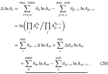
We use the same formula for total factor productivity growth as used by Solow (1957),
lnAINit −lnAINit−1=ln
wheresLit is the firm-specific fraction of the wage bill in output. For multilateral productivity level comparisons, Caves et al. (1982b) proposed an index in which each firm is compared with a hypothetical firm with average log output (lnQ), labor share (sL), and so on. The productivity level of firmiat timetis
lnAINit −lnAINt =(lnQit−lnQt)− ˜sit(lnLit−lnLt)
−(1− ˜sit)(lnKit−lnKt), (4)
with˜sit=(sLit+sLt)/2. This yields bilateral comparisons that are
transitive and still allows for technology that is firm-specific. The main advantages of the IN approach are the straight-forward computation (no estimation is required), the ability to
handle multiple outputs and many inputs, and the flexible and heterogeneous production technology that it allows. The main disadvantages are its deterministic nature and the required as-sumptions on firm behavior and market structure. Adjustments exist for regulated firms, noncompetitive output markets, and temporary equilibrium, but these either involve estimating some structural parameters or are more data-intensive.
2.2 Data Envelopment Analysis
Data envelopment analysis (DEA), or nonparametric frontier estimation, dates back to work of Farrell (1957). It was op-erationalized by Charnes, Cooper, and Rhodes (1978), and an overview of the method with applications has been provided by Seiford and Thrall (1990). No particular production function is assumed. Instead, productivity is defined as the ratio of a lin-ear combination of outputs over a linlin-ear combination of inputs. Observations that are not dominated are labeled 100% efficient. Domination occurs when another firm, or a linear combination of other firms, produces more of all outputs using the same input aggregate, where inputs are aggregated using the same weights.
A linear programming problem is solved separately for each observation. Input and output weights are chosen to maximize efficiency (productivity) for the unit under consideration. In ad-dition to sign restrictions, the efficiency of all other firms cannot exceed 100% when the same weights are applied to them. For unit 1 in the single-output case, the problem boils down to
max
vq,v∗,ul,uk
θ1=
vqQ1+v∗
ulL1+ukK1
subject to vqQj+v ∗
ulLj+ukKj
≤1, j=1, . . . ,N, (5) vq,ul+uk>0, ul,uk≥0.
Multiple outputs would be aggregated linearly, andv∗is a com-plementary slack variable to allow for variable returns to scale (v∗=0 for constant returns to scale). In practice, most applica-tions solve the dual problem, whereθ1is chosen directly.
The efficiency measureθi is estimated on a sample that
cludes all firm-years as separate observations and can be in-terpreted as the productivity difference between unitiand the most productive unit,θi=AAmaxi . Estimates of productivity
lev-els and growth rates that are comparable to those obtained with the other methodologies can be defined as
lnADEAit −lnADEAt =lnθit−
1 Nt
Nt
j=1
lnθjt (6)
and
lnADEAit −lnADEAit−1=lnθit−lnθit−1. (7)
These transformations do not change the ranking of firms, but that affect the absolute productivity levels and growth rates.
The main advantage of DEA is the absence of functional form or behavioral assumptions. The underlying technology is entirely unspecified and is allowed to vary across firms. The lin-ear aggregation is natural in an activities analysis framework. Each firm is considered a separate process that can be com-bined with others to replicate the production plan of the unit un-der investigation. On the other hand, the flexibility in weighting
has drawbacks. Each firm with the highest ratio for any output– input combination is 100% efficient. Under variable returns to scale, each firm with the lowest input or highest output level in absolute terms is also fully efficient. The most widely used im-plementations are not stochastic, making estimates sensitive to outliers. Because each observation is compared with all others, measurement error for a single firm can affect all productivity estimates.
2.3 Parametric Estimation
The parametric methods assume the same input trade-off and returns to scale for all firms. Functional form assumptions con-centrate all heterogeneity in the productivity term, but the ex-plicitly stochastic framework is likely to make estimates less susceptible to measurement error. We follow most of the lit-erature by estimating a Cobb–Douglas production function in logarithms,
qit=α0+αllit+αkkit+ωit+ǫit, (8)
whereωitrepresents a productivity difference known to the firm
but unobservable to the econometrician andǫit captures other
sources of iid error.
Consistent estimation of the input parameters faces an endo-geneity problem. Firms choose inputs knowing their own level of productivity, and a least squares regression of output on in-puts will give inconsistent estimates of the production function parameters. We implement three estimators that explicitly ad-dress the endogeneity problem. The two stochastic frontiers in Section 2.3.1 make explicit distributional assumptions on the unobserved productivity; the GMM–SYS estimator in Sec-tion 2.3.2 relies on instrumental variables, and the semipara-metric estimator in Section 2.3.3 inverts the investment func-tion nonparametrically to obtain an observable expression for productivity.
Because the input aggregator is assumed constant across time and firms, productivity level comparisons and growth rates are straightforward,
lnAzit−lnAzt=(qit−qt)− ˆαlz(lit−lt)− ˆαzk(kit−kt) (9)
and
lnAzit−lnAzit−1=(qit−qit−1)− ˆαzl(lit−lit−1)
− ˆαkz(kit−kit−1), (10)
z∈ {SF1,GMM,OP}. To obtain a clean estimate ofωit, an
esti-mate for the difference in error terms from the right side should be subtracted. Generally this is not possible and is ignored be-causeE(ǫit)=0. For the second stochastic frontier estimator
(SF2), a different formula is used to purge the random noise (ǫ) from the productivity estimates.
2.3.1 Parametric Estimation: Stochastic Frontiers. The stochastic frontier (SF) literature uses assumptions on the dis-tribution of the unobserved productivity component to sep-arate it from the random error. The method is credited to Aigner, Lovell, and Schmidt (1977) and Meeusen and van den Broeck (1977), who modeled productivity as a stochastic draw from the negative of an exponential or half-normal distribu-tion. Estimation is usually with maximum likelihood. In the production function (8), the term ωit is weakly negative and
interpreted as the inefficiency of firmiat timetrelative to the
best-practice production frontier. An alternative interpretation is that the firm-specific production function liesωit below best
practice.
Initially developed to measure productivity in a cross-section of firms, the model was generalized for panel data in a number of ways. Battese and Coelli (1992) provided the most straight-forward but also the most restrictive generalization, modeling the inefficiency term as
ωSFit 1= −eη(t−t0)ω
i withωi∼N+(γ , σ2). (11)
The relative productivity of each firm (ωi) is a time-invariant
draw from a truncated normal distribution. Inefficiency in-creases (dein-creases) deterministically over time ifηis positive (negative) at the same rate for all firms.
A more flexible generalization of the cross-sectional stochas-tic frontier, by Cornwell, Schmidt, and Sickles (1990), is to esti-mate a time-varying firm-specific effect using three coefficients per firm,
ωSF2it =αi0+αi1t+αi2t2. (12)
Productivity still evolves deterministically, but the growth rate changes over time and varies by firm.
Although it is customary to calculate technical inefficiency as E(eωit| ˆω
it+ ˆǫit), for comparability with the other methods, we
use the expected value of log productivity. For SF1, this boils down to the earlier formulas (9) and (10), because the best esti-mate ofE(ωit| ˆωit+ ˆǫit)is(ωˆit+ ˆǫit)ifωitis independent ofǫit.
For SF2, productivity level and growth can be calculated as
lnASF2it −lnASF2t =(αˆi0− ˆα0)+(αˆi1− ˆα1)t+(αˆi2− ˆα2)t2 (13)
and
lnASF2it −lnASF2it−1=(αˆi1− ˆαi2)+2αˆi2t. (14)
An advantage of the stochastic frontiers is that the deter-ministic part of the production function can be easily gener-alized to allow more sophisticated specifications, for exam-ple, to incorporate factor bias in technological change. They straightforwardly generalize the popular fixed-effects estima-tor. The two implementations trade-off flexibility in the char-acterization of productivity with estimation precision. SF2 uses 3×Ndegrees of freedom and is the only estimator for which consistency relies on asymptotics in the time dimension. One might also be uncomfortable with identification coming solely from distributional assumptions, which are especially restric-tive for SF1.
2.3.2 Parametric Estimation: Instrumental Variables (GMM). The general approach to estimating the dynamic er-ror component models of Blundell and Bond (1998) was first applied to production functions by Blundell and Bond (2000). The productivity term is modeled as a firm fixed effect (ωi)
plus an autoregressive component (ωit′ =ρω′it−1+ηit).
Quasi-differencing the production function gives the estimating equa-tion in its dynamic representaequa-tion,
qit=ρqit−1+αl(lit−ρlit−1)+αk(kit−ρkit−1)
+α′t+ωi′+(ηit+ǫit−ρǫit−1).
εit
(15)
There is still a need for moment conditions to provide instru-ments, because the inputs will be correlated with the composite errorεit.
Estimating equation (15) in first-differenced form takes care of the firm fixed effects. Three and more periods lagged inputs and output will be uncorrelated withεit under standard
exo-geneity assumptions on the initial conditions. At least three lags are necessary, becauseεitcontains errors as far back asǫit−2.
Blundell and Bond (1998) illustrated theoretically and with a practical application that these instruments can be weak. If one is willing to make the additional assumption that input changes are uncorrelated with the firm fixed effects, then twice-lagged first differences of inputs are valid instruments for the produc-tion funcproduc-tion in levels. The producproduc-tion funcproduc-tion in first differ-ences and levels are estimated jointly as a system with the ap-propriate set of instruments for each equation. Productivity is again calculated using (9) and (10).
The GMM–SYS method is flexible in generating instruments and allows testing for overidentification. It provides an autore-gressive component to productivity, in addition to a fixed com-ponent and an idiosyncratic comcom-ponent. Relative to the simple fixed-effects estimator, it also uses the information contained in the levels, which is likely to help with measurement error (see Griliches and Mairesse 1998). The main disadvantage is the need for a long panel; at least four time periods are required. Moreover, if instruments are weak, then the method risks under-estimating the coefficients.
2.3.3 Semiparametric Estimation (OP). This method was introduced by Olley and Pakes (1996) to estimate productivity effects of restructuring in the U.S. telecommunications equip-ment industry. Productivity, a state variable of the firm, is as-sumed to follow a Markov process unaffected by the control variables. Investment, a monotonically increasing function of productivity, becomes part of the capital stock with a one-period lag. Inverting the investment equation nonparametrically pro-vides an observable expression for the productivity term that can be used to substitute it from the production function. The methodology is more general than this exposition suggests. The basic idea is to use another decision by the firm to provide ad-ditional information on the unobserved productivity term. Al-ternatively, Levinsohn and Petrin (2003) inverted the material input demand.
In a first estimation step, the variable input coefficients and the joint effect of all state variables are estimated. In a sec-ond step, the coefficients on the observable state variables—just capital in our case—are identified, relying on the orthogonality of capital and the innovation in productivity. An intermediate step controls for sample selection, because firms are assumed to exit if productivity falls below a threshold, which is likely to be decreasing in capital. The probability of survival (P) isˆ predicted from a probit regression and will enter as a second ar-gument in the nonparametric functionψ (·)in the second step. The estimating equations for the two steps are
qit=α0+αllit+φt(iit,kit)+ǫit1 (16)
and
qit− ˆαllit=αkkit+ψ (φˆit−1−αkkit−1,Pˆit)+ǫit2. (17)
The functionsφtandψare approximated nonparametrically by
a fourth-order polynomial or a kernel density. Productivity is calculated from (9) and (10).
An advantage of the Olley–Pakes (OP) approach is the flexible characterization of productivity, assuming only that it evolves according to a Markov process. Potential weak-nesses are the nonparametric approximations. The functions that are inverted are complicated mappings from states to ac-tions, which must hold for all firms regardless of their size or competitive position. Ackerberg, Caves, and Frazer (2005) also illustrated that the implicit assumptions required to identify the variable input coefficients are relatively restrictive.
3. DATA
We evaluate the different methodologies using two datasets that have been used extensively in the productivity literature. The first of these is a panel of manufacturing plants from the Colombian Census of Manufacturers. (For a detailed descrip-tion of the data and variable construcdescrip-tion, see Roberts 1996.) It covers all active establishments between 1977 and 1991, but we limit the sample to plants that at some point are classified in the ISIC (rev. 2) industry 322, Clothing and Apparel. Plants in this industry are expected to be relatively homogeneous in technol-ogy, at least compared with other industries. The sector also has a relatively large foreign exposure, which makes it an interest-ing place to evaluate the different debates. In the final year of the sample, the textile industry accounts for 10% of manufac-turing employment, 3% of value added, and 8% of Colombian manufacturing exports.
The sample is further limited by including only plants that operate for at least 3 years, because many estimation meth-ods require at least three observations per plant. This results in an unbalanced panel of 14,348 observations from 1,957 plants with nonmissing information on output, labor, capital, wages,
and investment (investment is often zero). The output concept used is value added, defined as sales minus indirect costs and material input. Labor input is total employment, and capital in-put is the reported book value of the plant and equipment. Value added is deflated with the same sectoral output deflator used by Roberts (1996). For capital, the capital goods deflator from the IMF financial tables is used.
The second dataset contains a sample of manufacturing firms in Zimbabwe. Data were collected from firm surveys for 1993, 1994, and 1995. Approximately 200 firms were interviewed in three consecutive years. (For details on the sampling frame, the size distribution of firms, and some background information on the country, see Van Biesebroeck 2005b.) Firms come from four broadly defined manufacturing sectors: food, textile, wood, and metal, corresponding roughly to ISIC classifications 31, 32, 33, and 38. Some firms exited the sample each year, and new firms were added in later rounds to maintain the sample size. The short sample period required some modifications to the esti-mation algorithms. The SF2 estimator uses only a linear time trend, estimating firm-specific intercepts and growth rates, but no quadratic effects; the GMM estimator does not include firm dummies.
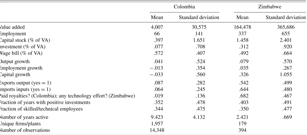
As before, only firms with nonmissing data on output, in-puts, wage bill, and investment (including zeros) are retained. Output is value added (sales minus indirect costs and mater-ial input), and inputs are total employment (labor) and the re-ported replacement value of the plant and equipment (capital). Value added and capital are deflated using the manufacturing deflator from the IMF financial tables. Table 1 contains some summary statistics. In all tables, results for Colombia are on the left and those for Zimbabwe are on the right. Note that the Colombian dataset covers plants and the Zimbabwean dataset covers firms; for ease of exposition, we occasionally use the terms “plants” and “firms” interchangeably to denote observa-tions in both datasets.
Table 1. Summary statistics
Colombia Zimbabwe
Mean Standard deviation Mean Standard deviation
Value added 4,007 30,575 164,478 365,686
Employment 66 141 337 655
Capital stock (% of VA) .397 1.651 1.458 2.401
Investment (% of VA) .077 .708 .312 .920
Wage bill (% of VA) .572 .407 .492 .664
Output growth .041 .524 .079 .570
Employment growth −.013 .354 .035 .267
Capital growth −.033 .560 .326 1.055
Exports output (yes=1) .087 .282 .542 .499
Imports inputs (yes=1) .064 .245 .644 .480
Paid royalties? (Colombia); any technology effort? (Zimbabwe) .019 .136 .682 .467 Fraction of years with positive investments .352 .478 .403 .491 Fraction of skilled/technical employees .344 .475 .350 .477
Number of years active 9.423 4.132 2.421 .669
Unique firms/plants 1,957 179
Number of observations 14,348 394
NOTE: For more information on the datasets see the work of Roberts (1996) for Colombia and that of Van Biesebroeck (2005b) for Zimbabwe.
4. DIRECT COMPARISON OF METHODOLOGIES
The following table summarizes the acronyms used when discussing the results and indicates the equations used to cal-culate productivity levels and growth rates:
Method (Level)−(Growth)
IN Törnqvist index enforcing constant returns to scale
(4)−(3)
DEA Data envelopment analysis: non-parametric frontier
(6)−(7)
SF1 Stochastic frontier with time-invariant productivity ranking
(9)−(10)
SF2 Stochastic frontier with two/three sets of dummies per firm
(13)−(14)
GMM Joint estimation of production func-tion in levels and first differences
(9)−(10)
OP Semiparametric inversion of invest-ment equation
(9)−(10)
NOTE: The index number calculations and semiparametric and SF2 estimation were pro-grammed in STATA. DEA estimation was carried out with software developed by the Op-erations Research and Systems Group at the Warwick Business School (Windows version 1.10). SF1 calculations are performed with the FRONTIER 4.1 program written by Tim Coelli, available athttp://www.uq.edu.au/economics/cepa/frontier.htm.The system GMM estimator was implemented using the GAUSS program DPD98 written by Manuel Arel-lano, available athttp://www.cemfi.es/˜arellano/#dpd.
4.1 Production Function Parameters
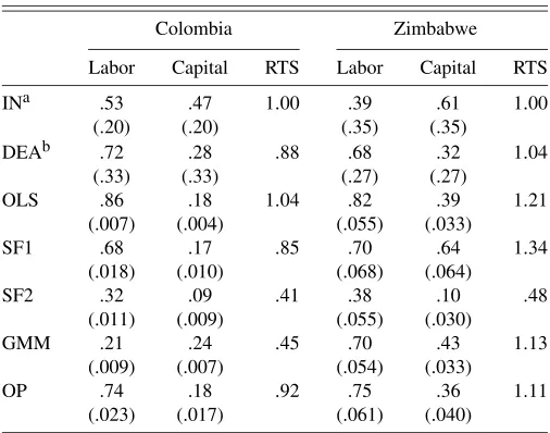
Table 2 lists the parametric estimates for the production func-tion coefficients with standard errors. For comparison, we also include ordinary least squares (OLS) estimates of the produc-tion funcproduc-tion. For the Törnqvist index, which allows for hetero-geneity in technology, the average wage bill in value added is reported in the labor column, with its standard deviation across
Table 2. Input coefficient estimates
Colombia Zimbabwe
Labor Capital RTS Labor Capital RTS
INa .53 .47 1.00 .39 .61 1.00
NOTE: For the parametric methods the coefficient estimates are reported with standard errors in parentheses. (RTS stands for returns to scale.)
aThe labor coefficient for IN is the average wage bill as a fraction of value added; the capital coefficient is 1−labor coefficient. The standard deviations over the entire sample are in parentheses.
bFor DEA, the median of the relative input weights and the median returns to scale are reported; standard deviations are in parentheses.
all observations. For the DEA results, we calculate the relative weight of labor and capital in the output aggregate and show the median and standard deviation of the distribution.
One choice to make is whether or not to enforce constant re-turns to scale (CRS). The CRS results for Colombia tend to be relatively similar for the different parametric methods; labor co-efficient estimates range from .75 to .80, and capital coco-efficient estimates are .20–.29. Full results are reported in the working paper version (Van Biesebroeck 2003). All labor coefficients are estimated <.83, and the capital coefficients are >.17, the respective OLS estimates. However, when returns to scale are estimated freely, all four parametric methods find them to be strongly and statistically significantly decreasing in the Colom-bian textile industry. For Zimbabwe, three parametric estima-tors find increasing returns to scale, whereas only the SF2 es-timator points to decreasing returns to scale. DEA allows the returns to scale to vary by firm, and the range of estimates is large (the standard deviation is .33 in Colombia and .32 in Zim-babwe). The median estimate is .88 for Colombia and 1.04 for Zimbabwe, broadly consistent with the parametric estimates.
In the absence of a priori evidence on scale economies, we do not impose them to be constant (except for the IN). Although the absolute size of scale economies differs, all estimators agree that the average plant in the Colombian textile sector has ex-hausted all scale economies and might even be operating above efficient scale. On the other hand, all but one estimator suggests that there are moderate scale economies left to be exploited by Zimbabwean manufacturing firms, consistent with the evidence presented by Tybout (2000). The different unit of analysis and the oversampling of large firms in Zimbabwe, makes it difficult to compare the two samples. It is noteworthy that the median textile firm in Zimbabwe uses only one-third as many work-ers as the median firm in the other industries, consistent with a much lower minimum efficient scale in textiles.
Accounting for the simultaneity of inputs and productivity lowers the labor coefficient estimate significantly for the para-metric methods relative to the OLS estimates. The two nonpara-metric methods also calculate an average weight for labor that is far below the OLS estimates. The range of estimates across the different methods is extremely wide in both samples, rang-ing from an implausibly low from .21 (GMM) to .74 (OP) in Colombia and from .38 (SF2) to .75 (OP) in Zimbabwe. Al-though the methods agree that OLS estimates are biased up-ward, there is no agreement whatsoever as to the true labor co-efficient. Moreover, the low standard errors convey a mislead-ing sense of accuracy.
The capital coefficient estimate is less affected by the si-multaneity correction, but the change relative to the OLS esti-mate can go in either direction. The SF1 estimator even finds a change in opposite directions in both datasets (relative to OLS). The range for the capital coefficient is even wider than for la-bor, ranging from .09 (SF2) to .47 (IN) in Colombia and from .10 (SF2) to .64 (SF1) in Zimbabwe.
Although the range of estimates is large, not all results are equally reliable. One notable pattern is that estimators that in-clude fixed effects (SF2 in both countries and GMM in Colom-bia) find strongly decreasing returns to scale. SF2 estimates of the coefficient on the capital stock, which tends to be relatively constant over time, are extremely low. The GMM capital coef-ficient estimate is higher, because lagged values of inputs are
relatively strong instruments for the capital stock. Griliches and Mairesse (1998) argued that the signal-to-noise ratio in the data is much reduced if input coefficients are identified from the changes over time, with measurement error biasing the coef-ficient estimates downward. In earlier work (Van Biesebroeck 2006), we used simulated data to show that measurement error can be a severe problem in these models.
Of the remaining estimates, the average wage bill (IN) is be-low all parametrically estimated labor coefficients. For devel-oping countries, this is not entirely surprising. To the extent that the production technology and machinery is imported from more developed countries and input substitution is limited, the capital intensity will be higher than optimal, given the low rel-ative factor price for labor. In addition, a substantial fraction of worker compensation might be in the form of nonwage benefits. Thus the wage bill will underestimate the share of labor in to-tal costs. Both phenomenons are likely to be more pronounced for Zimbabwe than for Colombia, which is consistent with the relative size of the average wage shares.
Finally, the SF1 assumption that all firms improve produc-tivity at the same rate is likely to be less appropriate in Zim-babwe than in Colombia. In the first 2 years of the sample, half of all Colombian plants experienced labor productivity growth between−.03 and .34; the comparable range for Zimbabwean firms was−.21 to .29, or 33% wider. Comparing the average firm-level growth rates over the entire sample periods in the two countries, the difference is even larger. Half of all Colom-bian plants averaged labor productivity growth between−.03 and .11; the comparable range for Zimbabwe is −.17 to .30, more than three times as wide.
Limiting attention to the three most reliable estimates for each country, the results are much more consistent. For Colom-bia, the labor elasticity is estimated at .68 with SF1 and .74 with OP; the interquartile range for the relative weight of labor with DEA is .54–.88. The three methods also find returns to scale to be decreasing in the range of .85–.92. For Zimbabwe, the labor coefficient is estimated rather similar, .70 by GMM and .75 by OP; DEA gives an interquartile range of .50–.84. The differ-ence in capital elasticities between the two countries is larger: the average is .21 for Colombia and .37 for Zimbabwe. As a result, returns to scale are estimated to be increasing in Zim-babwe, with an average point estimate of 1.09, and decreasing in Colombia, with an average of .88.
It is comforting to know that the large differences in Table 2 can be understood and that the range of most trustworthy es-timates is relatively narrow. However, these ex post insights when the entire range of estimates is available are not very use-ful from a practical perspective. Generally, only a single esti-mate is available, and one must decide whether or not to trust it. For each method, a number of diagnostics exist to judge the reliability of the results. For example, almost 10% of firms in Zimbabwe report a wage share higher than 1, but only 4% in Colombia do so, providing even more reason to not rely on the IN results in Zimbabwe. For DEA, we can check what fraction of observations are deemed 100% efficient. In both datasets, 20 observations are found to be fully efficient, which repre-sents 5.1% of all firms in Zimbabwe but only .14% of plants in Colombia. On the other hand, only 4.5% of observations in Zimbabwe construct an input aggregate by putting full weight
on a single input (almost always labor); this occurs for 15.6% of the observations in Colombia (split almost equally between capital and labor).
For the two stochastic frontiers, there are no obvious diagnos-tic checks, because they are not identified if the distributional assumptions are violated. We do find, however, that the esti-mated residuals of both the SF1 and SF2 models seem to follow an AR(1) process, which violates the models’ assumptions. For the GMM–SYS estimator, the restrictions on the parameters of the dynamic representation of the production function (e.g., the parameter on lagged capital should equal−ραk) are violated
in both countries, and we do not impose them. In Colombia, the overidentifying restrictions on the instruments are narrowly rejected, and there is strong evidence of serial correlations of more than one period. In the short panel available for Zim-babwe, the GMM–SYS estimation reduces to a cross-sectional system, and neither of these tests can be performed. For the OP estimation, a crude check is to verify graphically whether the monotonicity assumption between investment and tivity, conditional on capital, holds for the estimated produc-tivity series. This is the case for Colombia, but for Zimbabwe the surface curves up for low levels of investment (especially at high capital levels). A more formal test for the validity of the nonparametric inversions is to verify whether lagged labor input has any predictive power in the second-stage regression. For Colombia, the sample had to be split in three periods, based on the business cycle, with separate inversions performed over each period, for the coefficient to become insignificant. In Zim-babwe, the coefficient was significant with apvalue of .04.
Although these tests do raise a number of flags, these con-cerns are unlikely to be sufficiently alarming to reject any of the methodologies if only one set of results was available. The large differences in the observable component of the produc-tion funcproduc-tion has important consequences for any applicaproduc-tion that uses the production function directly as a representation of technology. For example, the potential effect of a trade policy that eliminates capital controls and attracts more FDI obviously will depend on the capital coefficient estimate. The estimated input coefficients allow for a decomposition of output differ-ences in observable input differdiffer-ences and a residual. Whether or not the residuals are deemed similar depends crucially on the fraction of the total output variation that can be explained by input differences. This is investigated in detail in the next two sections.
4.2 Productivity-Level Estimates
One way to compare the productivity estimates is by the dispersion that they imply. The first two columns in Table 3 contain the interquartile range for each method for Colombia, and columns (1b) and (2b) contain the same statistics for Zim-babwe. The median is normalized to zero by year. The widths of the intervals are relatively similar across rows, especially in Colombia, which is remarkable because the methods rely on very different calculations and assumptions. In each coun-try, the most narrow interval is about two-thirds as wide as the widest interval. Intervals are almost 50% wider in Zimbabwe than in Colombia, and the difference goes the same way for every method. It could be the result of the lower level of devel-opment or simply of the much smaller sample size.
Table 3. Productivity-level and growth estimates
Colombia Zimbabwe
Productivity level, Productivity growth, Productivity level, Productivity growth, interquartile range average interquartile range average
25th% 75th% Unweighted Weighted 25th% 75th% Unweighted Weighted
(1a) (2a) (3a) (4a) (1b) (2b) (3b) (4b)
IN −.413 .382 .062 .088 −.387 .742 −.136 −.336 DEA −.498 .522 .065 .106 −.535 .618 −.074 −.042 SF1 −.360 .340 .060 .121 −.726 .631 −.133 −.273 SF2 −.566 .457 .049 .054 −.399 1.278 .024 .037 GMM −.542 .491 .057 .120 −.499 .547 −.080 −.141 OP −.337 .319 .061 .121 −.503 .554 −.061 −.101
NOTE: The quartiles for productivity level are for the entire sample, pooling all plant-year (Colombia) or firm-year (Zimbabwe) observations, normalizing productivity by the median for the year. The average productivity growth statistics are also calculated over the entire sample and output weights (by year) are used when weighing.
The methods that estimate large decreasing returns to scale (SF2 in both countries and GMM in Colombia) also find the widest intervals of all methods. In Colombia, the two nonpara-metric methods that allow heterogeneity in technology (IN and DEA) also tend to find somewhat wider intervals, but the differ-ence is less pronounced in Zimbabwe. In general, productivity is highly dispersed. Even in Colombia, only half of all plants have a productivity level between 45% below and 42% above the median.
Most methods find a distribution of productivity that is slightly skewed to the left in Colombia and more noticeably right-skewed in Zimbabwe. The right-skewness in Zimbabwe is consistent with the OP model of competitive selection (Olley
and Pakes 1996); firms exit when their productivity drops below a threshold, truncating the distribution from the left. The SF1 methodology, which has left-skewness built-in—productivity is the sum of a symmetric normal error and an inefficiency term that follows a normal distribution truncated from the right—is the only method to find left-skewness in Zimbabwe. In Colom-bia, only the DEA method finds right-skewness, the opposite of all other methods.
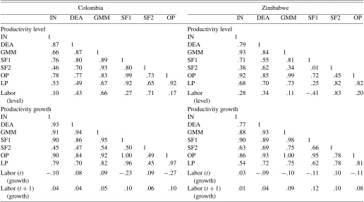
A second way to compare the productivity estimates is to look at the correlations between the different measures directly. For Colombia, in the top left panel of Table 4, the average cor-relation is .79, and even .86 limiting the comparison to the para-metric methods. Even DEA, which leaves technology entirely
Table 4. Correlations between different productivity level and growth estimates
Colombia Zimbabwe
IN DEA GMM SF1 SF2 OP IN DEA GMM SF1 SF2 OP
Productivity level Productivity level
IN 1 IN 1
DEA .87 1 DEA .79 1
GMM .66 .87 1 GMM .93 .84 1
SF1 .76 .80 .89 1 SF1 .71 .55 .81 1
SF2 .46 .70 .93 .80 1 SF2 .38 .62 .34 .01 1 OP .78 .77 .83 .99 .73 1 OP .92 .85 .99 .72 .45 1 LP .53 .49 .67 .92 .65 .92 LP .68 .70 .73 .25 .82 .82
Labor (level)
.10 .43 .66 .27 .71 .17 Labor (level)
.28 .34 .11 −.41 .83 .20
Productivity growth Productivity growth
IN 1 IN 1
DEA .93 1 DEA .77 1
GMM .91 .94 1 GMM .88 .93 1
SF1 .90 .86 .95 1 SF1 .90 .89 .98 1
SF2 .45 .47 .54 .50 1 SF2 .63 .69 .75 .66 1 OP .90 .84 .92 1.00 .49 1 OP .86 .93 1.00 .95 .78 1 LP .79 .70 .82 .96 .45 .97 LP .54 .72 .75 .62 .78 .81 Labor (t)
(growth)
−.10 .08 .09 −.23 .09 −.27 Labor (t) (growth)
.03 −.09 −.10 −.11 .10 −.11
Labor (t+1) (growth)
.04 .04 .05 .10 .06 .10 Labor (t+1) (growth)
.01 .04 .09 .12 .10 .08
NOTE: Partial correlation statistics between the different (log) productivity measures and between productivity and labor input; correlations are calculated across all observations (plant/firm−years). The bottom row reports the correlation between labor input growth and one period lagged productivity.
unspecified, or GMM, which estimates returns to scale to be very low, produce productivity estimates very similar to those of the other methods. Only the correlation between the SF2 and IN productivity estimates is below .50. Imposing constant re-turns to scale, the correlations are even higher; the lowest cor-relation is .79. The results for Zimbabwe are broadly similar. The average correlation is lower (.66), but this is driven largely by the more dissimilar results for SF2. Omitting this estimator, which estimates two firm-specific coefficients from only 3 years of data, raises the average correlation to .86.
For comparison, we also added correlations between labor productivity (LP), defined as value added per worker, and the different multifactor productivity measures. Only in a single in-stance (correlations with the DEA estimates in Colombia) is the correlation with labor productivity lower than with all the other measures. In Colombia, correlations of either SF1 or OP with each alternative productivity measure always exceed cor-relations with LP, but both of these measures achieve a very high correlation with LP themselves (.92). In Zimbabwe, cor-relations with LP are never the lowest, and no method achieves consistently higher correlations with the others than LP.
The broad similarity of the productivity estimates across methods, despite of the large differences in input coefficient es-timates, indicates that the variation in the observable part of the production function is swamped by variation in unobservables. Even labor productivity estimates are surprisingly similar. Only the SF2 results—which purge the random errors [ǫ in eq. (8)] from the productivity estimates—are noticeably different from the other results in Zimbabwe. If one is interested only in the productivity residuals and not in the input coefficients or scale economies, then the choice of methodology turns out to be of secondary importance.
4.3 Productivity Growth Estimates
To compare the productivity growth estimates, Table 3 lists the unweighted and output-weighted averages of productiv-ity growth across all observations in each sample. The period 1977–1991 was clearly a very successful period for Colombian textile plants. The unweighted average (real) growth rate across all methods is 5.9% per year. By any standard, this is extremely rapid multifactor productivity growth. At the same time, the differences between productivity measures are small. The one method that takes out measurement error (SF2) produces the lowest estimate, which is still 4.9%. All other methods produce an estimate in the 5.7–6.5% range.
In Zimbabwe, the differences are larger. The average is now
−7.7%, and the estimates range from−13.6% to+2.4%. The only positive average is for SF2, which estimates a constant (deterministic) growth rate per firm based on at most 3 years of data. Moreover, it calculates the average growth rate based only on the limited sample of firms observed in each of the 3 years, and one would expect survivors to be more successful. Without this outlier, the average is −9.7%, and all estimates are in the−13.6% to−6.1% range, clearly a dismal period for productivity growth in Zimbabwean manufacturing.
Weighing the growth rates by plant output level increases the average productivity growth in Colombia for each method. This is as expected; plants with high output at the end period receive
a higher weight and tend to have, ceteris paribus, higher pro-ductivity growth. For Zimbabwe, the same effect is consistent with a higher average growth rate for the DEA or SF2 results if output weights are used. Results for the other methods go in the opposite direction; that is, weighting lowers the average. This can be explained by the increasing returns to scale technology that the SF1, GMM, and OP methods estimate; in a declining economy, larger firms are penalized additionally. In both coun-tries, the differences between the methods are exacerbated by weighting, and the SF2 method is now even more of an out-lier. Nevertheless, the main conclusion is the same using each productivity measure: Colombian textile plants were extremely successful over the sample period, and Zimbabwean manufac-turing firms were extremely unsuccessful.
The correlations between the different productivity growth estimates, given in the bottom panels of Table 4, mirror the patterns in the level correlations; in particular, correlations be-tween the GMM, SF1, and OP results are extremely high. En-forcing constant returns to scale (see Van Biesebroeck 2003) makes them virtually identical. The much lower estimate for scale economies by GMM in Colombia does not result in less well-correlated productivity growth estimates. Even the non-parametric DEA and IN results are very similar to the paramet-ric results. Except for the correlations with the SF2 measures, which are the clear outliers in both countries, the lowest cor-relation statistic for Colombia is .84, and that for Zimbabwe it is .77. The average correlations are .77 for Colombia and .84 for Zimbabwe and are even .92 and .91 when omitting the SF2 results.
Finally, the bottom of each panel in Table 4 reports the corre-lation statistics between productivity estimates and labor input. Such measures are sometimes calculated in macroeconomics to study the covariance between technology and inputs (see, e.g., Basu, Fernald, and Kimball 2006). In levels, the correla-tions indicate that larger plants (high employment) are on av-erage more productive, consistent with the higher wages that they generally pay. The correlations are especially large for the three measures that include fixed effects and are negative only for SF1 in Zimbabwe, as expected given the estimated re-turns to scale. More interesting are the correlations in growth rates. Several measures (SF1 and OP in both countries and IN in Colombia) find a significantly negative relationship between labor input growth and concurrent productivity growth, consis-tent with the evidence presented by Basu at al. (2006) at the aggregate level for U.S. manufacturing. Moreover, the corre-lations between lagged productivity growth and labor growth, the bottom row in Table 4, are positive and similar in size for all measures in both countries. They suggest that productivity growth, as a proxy for technology improvements, leads to fu-ture expansions, again consistent with the findings Basu et al. (2006).
Even though the relative importance attached to the different inputs varies substantially among methods, the impact on pro-ductivity estimates is limited. The differences in input coeffi-cients are swamped by the huge differences in output and input growth rates across firms. Productivity growth rates across the different methods are even more similar than the productivity levels. The similarity between the nonparametric and paramet-ric results is especially remarkable. The principal reason for this
is that the correlation of the growth rates of capital and labor across firms exceeds the corresponding correlation for the in-put levels. This is highlighted by the high correlations obtained between most measures and labor productivity growth. The one exception is SF2; these estimates are similar to the others for productivity levels, but not for growth rates.
The direct comparison of productivity measures showed surprisingly similar estimates for the different methods. The second approach to evaluate the importance of measurement methodology is to verify whether the conclusions on the three productivity debates are more sensitive to the choice of produc-tivity estimator.
5. THREE DEBATES
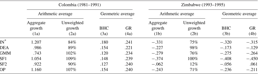
5.1 Does Learning-by-Exporting Increase Productivity?
The first question—whether firms that export are able to crease their productivity level—has been one of the most in-tensely researched questions in the productivity literature for a decade. Whereas it is well established that exporters have higher productivity than nonexporters (see, e.g., Bernard and Jensen 1995; Aw, Chung, and Roberts 2000), causality could go either way. A first channel is the self-selection of more pro-ductive firms into the export market. Possibly, exporters do not derive any productivity gains from this activity, and their pro-ductivity advantage could be fully established before they start exporting. Future exporters have been found to differ on many dimensions from nonexporters, even before they start exporting. Self-selection is certain to explain at least part of the observed correlation between export status and productivity level. Lopez (2005) surveyed the literature and noted that each microeco-nomic study finds support for such an effect.
An additional causal effect could go in the other direction if exporters are able to increase their productivity level as they learn from their export activities. Such a learning-by-exporting effect is not mutually exclusive with self-selection, but estab-lishing its existence has important policy implications. Trade liberalization is often promoted as a stimulus to raise productiv-ity levels; the domestic industry will have to face foreign com-petition at home and (should firms choose to export) abroad. Hard evidence for such an effect was virtually nonexistent un-til recently. Moreover, the earliest rigorous studies looking for learning-by-exporting effects did not find any. For example, Clerides et al. (1998) and Bernard and Jensen (1999) found for Colombia, Morocco, and the United States that the posi-tive correlation between productivity and export status can be explained entirely by self-selection. Later studies, starting with that of Kraay (1999) for China, did find learning effects, but they often come with caveats: only in certain industries, only after a longer spell on the export market, or only in the first 1 or 2 years.
Lopez (2005) provided an extensive list of additional stud-ies concluding against (e.g., in Spain, Germany, and South Ko-rea) or in favor of the learning-by-exporting hypothesis (e.g., for sub-Saharan Africa, the U.K., or Canada). From this litera-ture, it is difficult to gauge to what extent opposing conclusions reflect methodology or genuine economic differences between the countries. We test for a learning-by-exporting effect using
each of the productivity measures and two distinct approaches to control for firms self-selecting into the export market.
First, we estimate a simultaneous equation model similar to that of Clerides et al. (1998),
lnAit=
A probit model of a firm’s export decision [eq. (19)] is es-timated jointly with (18), which represents the evolution of productivity. Two lags of export status and productivity are included in each equation. The lagged productivity terms in (18) capture persistence in productivity; in (19) they capture self-selection of more productive firms into the export market. Lagged export status in the probit equation captures export per-sistence resulting, for example, from sunk costs of exporting. The parameters of interest are those on lagged export status in the productivity equation,αx1andαx2, which will be positive if
past export experience has a beneficial effect on the current pro-ductivity level. Estimation follows Clerides et al. (1998). The persistent component in the unobservable (ω) is assumed to be normally distributed, allowed to be correlated across equations, and integrated out using Gaussian quadrature. In these and all other regressions in Table 5, employment and time, location, and industry dummies are included as controls.
The second approach to control for self-selection is with a matching estimator, as adopted by Wagner (2002) and De Loecker (2005). These authors found evidence of learning-by-exporting in Slovenia but not in Germany. A firm is considered “treated” the first year that it exports (if productivity in the fol-lowing year is observed). Each treated firm is matched with re-placement to a control, the nonexporter with the closest propen-sity score, that is, its “nearest neighbor.” The propenpropen-sity score is calculated as the predicted value from a probit regression of the treatment dummy on lagged productivity, employment, wages, and the same control dummies as before. The productivity pre-mium for exporters is estimated on the limited sample of treated and control firms by regressing log productivity 1 year post-treatment on the post-treatment dummy and controls. In the sam-ple for Zimbabwe, only four treated firms can be identified; in Colombia, there are 119 treated plants.
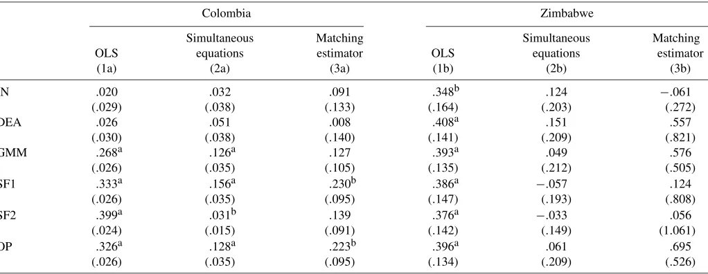
As a benchmark, columns (1a) and (1b) in Table 5 show the productivity premium for exporters from a simple least squares regression of log productivity on lagged export status and con-trols. Estimates for Zimbabwe are all in a narrow range between .348 and .408 and highly significant. For Colombia, the para-metric methods find similar premiums, between .268 and .399, but the nonparametric methods (IN and DEA) that allow dif-ferent input elasticities by plant find productivity premiums an order of magnitude smaller and not significantly different from zero. This is consistent with some earlier studies showing that exporters are not only larger, but also produce with a larger cap-ital stock per employee. Accounting nonparametrically for the higher capital intensity of exporters explains away most of the
Table 5. First debate: Learning-by-exporting
Colombia Zimbabwe
Simultaneous Matching Simultaneous Matching OLS equations estimator OLS equations estimator
(1a) (2a) (3a) (1b) (2b) (3b)
IN .020 .032 .091 .348b .124 −.061
(.029) (.038) (.133) (.164) (.203) (.272)
DEA .026 .051 .008 .408a .151 .557
(.030) (.038) (.140) (.141) (.209) (.821)
GMM .268a .126a .127 .393a .049 .576
(.026) (.035) (.105) (.135) (.212) (.505)
SF1 .333a .156a .230b .386a −.057 .124
(.026) (.035) (.095) (.147) (.193) (.808)
SF2 .399a .031b .139 .376a −.033 .056
(.024) (.015) (.091) (.142) (.149) (1.061)
OP .326a .128a .223b .396a .061 .695
(.026) (.035) (.095) (.134) (.209) (.526)
NOTE: The statistics reported are coefficient estimates and standard errors on the lagged export dummy in separate regressions with the different log productivity measures as dependent variables. Results in the first columns are for an OLS regression on the full sample, controlling for employment and time, location, and industry dummies. Statistics in the second column are coefficient estimates on once-lagged export status in the productivity equation, estimated by the simultaneous equation model of Clerides et al. (1998). Estimates in the third column are from a regression similar to the first column, but on the limited sample of treated (new exporters) and matched plants, using nearest-neighbor matching with replacement. The propensity score used in the match is estimated by a probit on lagged productivity, employment, and wages and time, location, and industry dummies.
aSignificant at the 1% level. bSignificant at the 5% level.
estimated productivity advantage. The difference in export par-ticipation helps explain the different results in the two countries. In the Colombian sample, fewer than 9% of the plants export and the parametrically estimated input coefficients will be more representative of the production technology of nonexporters. In the Zimbabwean sample, 54% of firms export and the produc-tion funcproduc-tion estimates will be more appropriate for exporters. The IN results produce the lowest estimate for the productivity premium of exporters in Zimbabwe as well, although the DEA estimate is at the other end of the spectrum.
Controlling for self-selection of more productive firms into the export market is expected to diminish the impact of ex-port status on productivity. Results for the simultaneous equa-tions approach—the coefficient on once-lagged export status in (18) is reported—are in columns (2a) and (2b) of Table 5. For Colombia, the point estimates for the parametric methods drop to one-third of the OLS estimates on average, but they remain significantly positive. For the two nonparametric meth-ods, estimates are similar to the OLS results and still insignif-icant. Under the maintained hypothesis that plants share the same production technology, one would conclude that learning-by-exporting effects are indeed present and are relatively large. The productivity premium is estimated at 11% on average.
However, the nonparametric results suggest that this conclu-sion is misleading, because they indicate a productivity pre-mium for exporters of only 4% on average, and the difference with nonexporters is not statistically significant. Notably, the study by Clerides et al. (1998)—one of the most prominent studies to find against the learning-by-exporting hypothesis— used an estimate of average variable cost, purged from capital-intensity effects in a flexible way, as a dependent variable.
For Zimbabwe, the range of estimates widens substantially. The point estimates vary from a productivity decline of−.057
(SF1) to an increase of .151 (DEA), but no longer is any esti-mate significantly different from 0. In contrast to the Colom-bian results, the nonparametric estimates are at the high end of the range. The large reduction in the point estimates in both countries relative to the OLS estimates in columns (1a) and (1b) points to important self-selection effects.
Estimates of the productivity premium using the matching estimator to control for self-selection are in columns (3a) and (3b). The results are very similar to the simultaneous equa-tion results. For Colombia, estimates are larger for the para-metric methods than for the nonparapara-metric methods, but only two methods still find significant learning effects. The point es-timates tend to be higher with the matching estimator, but the standard errors increase even more. For Zimbabwe, only four firms with data available in the year post-export can be identi-fied as new exporters. Five of the six point estimates are pos-itive, but the range is extremely wide, and the large standard errors do not hide the imprecision.
In sum, all methods find that exporters are more productive, but controlling for self-selection reduces the difference in most cases, especially for the parametric methods, and widens the range of point estimates across methods. The results for Zim-babwe all become insignificant, although some point estimates remain large. In Colombia, there is a significant learning effect if we assume that technology is homogeneous across plants, but the size of the premium is estimated to be much lower using the nonparametric methods. This is one instance when an im-portant assumption of the productivity measurement methodol-ogy crucially affects the results. A formal test for a structural break in the production function parameters between exporters and nonexporters strongly rejects that both groups operate with the same technology (see Van Biesebroeck 2005a for results in sub-Saharan Africa). The nonparametric methods estimate the position of a plant relative to other plants in the industry to be