IAS 29 and the cost of holding money under hyperinflationary conditions

(1)

This ar t icle was dow nloaded by: [ Univer sit as Dian Nuswant or o] , [ Rir ih Dian Prat iw i SE Msi] On: 29 Decem ber 2013, At : 19: 02

Publisher : Rout ledge

I nfor m a Lt d Regist er ed in England and Wales Regist er ed Num ber : 1072954 Regist er ed office: Mor t im er House, 37- 41 Mor t im er St r eet , London W1T 3JH, UK

Accounting and Business Research

Publ icat ion det ail s, incl uding inst ruct ions f or aut hors and subscript ion inf ormat ion:

ht t p: / / www. t andf onl ine. com/ l oi/ rabr20

IAS 29 and the cost of holding money under

hyperinflationary conditions

Andrew Higson a , Yoshikat su Shinozawa a & Mark Tippet t a a

Loughborough Universit y Publ ished onl ine: 28 Feb 2012.

To cite this article: Andrew Higson , Yoshikat su Shinozawa & Mark Tippet t (2007) IAS 29 and t he cost of hol ding money under hyperinf l at ionary condit ions, Account ing and Business Research, 37: 2, 97-121, DOI: 10. 1080/ 00014788. 2007. 9730064

To link to this article: ht t p: / / dx. doi. org/ 10. 1080/ 00014788. 2007. 9730064

PLEASE SCROLL DOWN FOR ARTI CLE

Taylor & Francis m akes ever y effor t t o ensur e t he accuracy of all t he infor m at ion ( t he “ Cont ent ” ) cont ained in t he publicat ions on our plat for m . How ever, Taylor & Francis, our agent s, and our licensor s m ake no r epr esent at ions or war rant ies w hat soever as t o t he accuracy, com plet eness, or suit abilit y for any pur pose of t he Cont ent . Any opinions and view s expr essed in t his publicat ion ar e t he opinions and view s of t he aut hor s, and ar e not t he view s of or endor sed by Taylor & Francis. The accuracy of t he Cont ent should not be r elied upon and should be independent ly ver ified w it h pr im ar y sour ces of infor m at ion. Taylor and Francis shall not be liable for any losses, act ions, claim s, pr oceedings, dem ands, cost s, expenses, dam ages, and ot her liabilit ies w hat soever or how soever caused ar ising dir ect ly or indir ect ly in connect ion w it h, in r elat ion t o or ar ising out of t he use of t he Cont ent .

(2)

Accounting

zyxwvutsrqponmlkjihgfedcbaZYXWVUTSRQPONMLKJIHGFEDCBA

ond Business Reseorch,

zyxwvutsrqponmlkjihgfedcbaZYXWVUTSRQPONMLKJIHGFEDCBA

Vol.

37. No. 2. pp.

97-121. 2007 97

IAS 29 and the cost of holding money

hyperinflationary conditions

Andrew Higson, Yoshikatsu Shinozawa and Mark Tippett*

under

Abstract -Empirical evidence is presented on the efficacy of procedures summarised in IAS 29: Financial Reporting in Hyperinjlarionary Economies for estimating the loss in purchasing power from holding monetary items during hyperinflationary periods. Our empirical analysis encompasses 32 hyperinflationary economies covering a wide variety of hyperinflationary conditions and spanning a period of more than 80 years. While the estimation procedures summarised in IAS 29 perform poorly under all the hyperinflationary conditions encompassed

by our sample, they are especially poor when the rate of inflation accelerates towards the end

zyxwvutsrqponmlkjihgfedcbaZYXWVUTSRQPONMLKJIHGFEDCBA

of a relatively short

hyperinflationary period. For these latter economies, our best estimate of the actual purchasing power loss is typi- cally only a small fraction of the figure obtained under the IAS 29 procedures. For hyperinflations of longer dura- tion, the IAS 29 procedures return estimated purchasing power losses that are typically around 10% larger than our best estimate of the actual losses. We also derive and empirically test a general class of ‘two point’ estimation formulae that make more efficient use of the sparse information set on which the IAS 29 estimation procedures are based. The results obtained from this procedure are encouraging and suggest it is possible to obtain reliable estimates of purchasing power losses using only sparse information sets provided realistic assumptions are made about the way monetary holdings respond to variations in the purchasing power of the currency.

Key words: Hyperinflation; IAS 29; monetary items; quadrature (estimating) formula; purchasing power loss.

1. Introduction

Seigniorage is the process whereby governments print currency and exchange it at face value for the goods and services required to implement their spending programmes. Governments generally en- sure that the rate of growth in the currency is roughly comparable with the rate of growth in general economic activity. However, there are numer-

ous instances of weak and/or insipid governments that have relied almost exclusively on seigniorage to finance their spending programmes. In these cases the rate of growth in the currency normally

far exceeds the rate of growth in general economic activity and the currency ends up being debased by hyperinflation. The most notorious example of this practice is provided by the German hyperinflation during the Weimar Republic after the First World War as it struggled to meet the reparation payments required of it under the Versailles Treaty. More recent examples of these hyperinflationary seigniorage practices are provided by Angola between 1996 and 2005, Belarus between 1995 and 2003, Madagascar between 1994 and 1996, Poland between 1990 and 1995, Romania between 1994 and 2002, Russia after the break-up of the Soviet Union in 1992, Turkey until the reform of the cur-

*Andrew Higson and Yoshikatsu Shinozawa are lecturers and Mark Tippett is Professor of Accounting and Finance at Loughborough University. Correspondence should be addressed to Mark Tippett at the Business School, Loughborough University, Leicestershire, LEI 1 3TU. E-mail: [email protected] .uk

This paper was accepted in February 2007.

rency in 2005 and the Ukraine between 1993 and 1997. Hence, it is not unusual to encounter organisations that have to operate under hyperinflationary conditions and the International Accounting Standards Board (IASB) has endorsed the finan- cial reporting standard IAS 29: Financial Reporting

in Hyperinflationary Economies (IASC, 1989) to

meet the unique financial reporting problems that arise in such environments.

IAS 29 does not establish an absolute rate of inflation at which hyperinflationary conditions will be deemed to prevail but instead sets out some general characteristics that indicate the presence of hyperinflation and under which the reporting pro- visions summarised in the standard are to be implemented. The characteristics include the ob- servation (para. 3) that the ‘general population’ prefers to maintain its wealth in non-monetary assets or in monetary assets denominated in a relatively stable foreign currency; that interest rates on debt transactions are linked to the rate of change in prices while credit sales and purchases are made at prices which compensate for the expected loss in purchasing power over the credit period; and that the cumulative rate of inflation over the previous three years is approaching or exceeds 100%. When these conditions are satisfied, para. 8 of IAS 29 mandates that published corporate financial statements ‘shall be stated in terms of the measur- ing unit current at the reporting date’. This means that the revenue and expense items appearing on

an organisation’s profit and loss statement will have to be restated by multiplying them by the

(3)

98

ratio of the general price index at the end of the reporting period to the general price index at the time when the revenue was received or expense incurred. Likewise, the fixed assets appearing on an organisation’s balance sheet will have to be restated by multiplying them by the ratio of the general price index at the balance sheet date to the general price index at the time when the fixed assets were

acquired. However,

zyxwvutsrqponmlkjihgfedcbaZYXWVUTSRQPONMLKJIHGFEDCBA

IAS 29 also notes that organi-

sations typically hold assets and liabilities denominated in the currency of the hyperinflationary economy (so called monetary assets and liabilities or monetary items) and these will rapidly decrease in purchasing power as the hyperinflation eats away at their nominal value. Given this, para. 9 of

IAS 29 also mandates that the net gain or loss in

purchasing power from holding these monetary assets and liabilities must be included in the organisation’s profit or loss and separately disclosed.

Unfortunately, IAS 29 provides only limited

guidance about how the gain or loss from holding these monetary items is to be estimated, suggest- ing instead that (para. 10) ‘consistent application

of these

zyxwvutsrqponmlkjihgfedcbaZYXWVUTSRQPONMLKJIHGFEDCBA

. . .

procedures and judgements’ employed in estimating the gain or loss in purchasing power

‘is more important than the precise accuracy of the resulting amounts included in the restated financial statements’. However, if shareholders and others are to make effective assessments about how well organisations have managed their monetary assets and liabilities and the purchasing power gains and losses that arise from them (both in ab-

ACCOUNTING AND BUSINESS RESEARCH

solute terms and in comparison with other organisations) then it is important that the gain or loss from holding monetary items reported on an organisation’s profit and loss statement be as accu- rate as possible.

This ‘consistency rather than accuracy’ principle that underscores the re-statement process sum- marked in IAS 29 no doubt informs the ‘illustra-

tive’ examples appended to the statement by those countries which have sought to make their domes- tic accounting standards compatible with the standards issued by the IASB. The estimation

procedures demonstrated in these illustrative examples are based on the premise that an organisation’s monetary position’ changes on just a few (typically, one or two) occasions over an annual reporting period and that in between these changes its monetary position remains constant.2 However, there is a long line of empirical work beginning with Cagan (1956) which shows that organisations rapidly adjust their holdings of monetary items as the rate of inflation gains momentum.’ In the German hyperinflation referred to earlier, for example, Cagan (1956: 102) shows that real monetary holdings declined by over 90% in the period from July 1922 until October 1923 as a consequence of a monthly inflation rate which grew from 43% in July 1922 to over of 3,773% by October 1923

.“

In such hyperinflationary environments, it is problematic whether an organisation’s monetary holdings over the reporting period can be captured by the one or two observations of that variable on which the IAS 29 estimation proce-

dures are invariably based, This in turn means that the IAS 29 estimation procedures will form an un-

reliable basis for assessing the efficiency (or otherwise) with which organisations manage the purchasing power gains and losses that arise on their monetary assets and liabilities.

Given this, our purpose here is twofold. First, we

use data from 32 hyperinflationary economies spanning an 80-year period to asses the relative efficiency of the procedures summarised in IAS 29

for estimating purchasing power gains and losses under a broad range of hyperinflationary environments. Our empirical analysis shows that the estimation procedures summarised in IAS 29 perform

poorly, but especially so when the rate of inflation accelerates towards the end of a relatively short hyperinflationary period. For these latter economies, our best estimate of the actual purchasing power loss is typically only a small fraction of the figure obtained under the IAS 29 procedures.

For hyperinflations of longer duration, the IAS 29

procedures return estimated purchasing power losses that are typically around 10% larger than our best estimate of the actual losses.

Our second contribution lies in the development of more sophisticated approaches for estimating

’

An organisation’s monetary position or equivalently its monetary items, is its monetary assets less its monetary liabilities. While an individual organisation’s monetary position can be positive or negative (depending on whether its monetary assets exceed its monetary liabilities) for the economy as a whole the aggregate monetary position must be negative since someone has to hold the currency issued by the government. See Lucas (2000:247) for further discussion of this point.

A good example of this practice is to be found in the numerical example appended to International Public Sector

Accounting Standard

zyxwvutsrqponmlkjihgfedcbaZYXWVUTSRQPONMLKJIHGFEDCBA

IPSAS

10:

Finoncia/ Reporting in

Hyperinflationary Economies which is available from the fol- lowing website:

http://www.ifac

.org/Members/Source_Files/Public_Sector/

IPSAS IO.PDF

Other countries which have adopted IASB standards have also followed this practice. For example, until recently the Australian Accounting Standards Board appended the IPSAS

10 numerical example to AASB 129: Financial Reporting in

Hy/xrinflationary Economies which is the Australian equiva- lent of IAS 29. AASB 129, complete with the IPSAS 10 numerical example, may be viewed at the following website:

http://www.comlaw.gov.au/ComLaw/Legislation/Legislative

Instrument 1

zyxwvutsrqponmlkjihgfedcbaZYXWVUTSRQPONMLKJIHGFEDCBA

.nsf/O/BF20E8CBE34CD250CA25700300244

CCA/$file/AASB 129-07-04c.pdf.

See Lucas (2000) for a summary of this literature. An organisation’s real monetary position is the book value of its monetary items divided by the price index used to calcu- late the gain or loss in purchasing power arising on its monetary items. It is, in other words, equivalent to the ‘purchasing power’ of the firm’s monetary items.

(4)

Vol. 37 No.

2. 2007

the purchasing power gains and losses that arise on monetary holdings. These more sophisticated procedures invoke the assumption that organisations rapidly adjust their monetary holdings as the rate of inflation gains momentum in contrast to the estimation procedures summarised in IAS 29, which make the unlikely assumption that organisations adjust their monetary holdings on just one or two occasions over a given hyperinflationary period. Moreover, our empirical analysis shows that the estimated purchasing power losses under these more sophisticated techniques are typically within 2.5% of our best estimate of the actual purchasing power losses. This result has the important implication that it is possible to obtain reliable estimates of purchasing power losses using only the sparse information set on which the IAS 29 estimation procedures are typically based provided realistic assumptions are made about the way organisations adjust their monetary holdings in response to variations in the purchasing power of the currency on issue.

We commence our analysis in the next section by summarising the numerical procedures we use for determining our ‘best estimates’ of the actual purchasing power losses that arise on the hyperinflationary economies employed in our empirical analysis. We then illustrate the practical application of these procedures by determining our best

estimates of the actual losses in purchasing power

zyxwvutsrqponmlkjihgfedcbaZYXWVUTSRQPONMLKJIHGFEDCBA

on the currency on issue for the US and the UK for

each year over the period from 1990 until 2005. Our calculations show that the procedures endorsed by IAS 29 return systematically biased estimates of the purchasing power losses on the currencies of both countries when compared to our best estimates of the actual purchasing power losses. Fortunately, the estimation errors are not partic- ularly large - typically, 3 4 % of our best estimate

of the actual figure. However, the systematic na- ture of the errors suggests that were the IAS 29 procedures to be applied to the data of hyperinflationary economies then errors of a considerably larger magnitude would be incurred. Section 3 ex- plores this latter issue in further detail by compar-

ing the estimated purchasing power losses for our

32 hyperinflationary economies under the IAS 29 procedures with our best estimate of the actual purchasing power losses. In Section 4 we derive and then empirically evaluate a general class of ‘two-point’ estimation formulae that make more efficient use of the sparse information set on which the IAS 29 estimation procedures are typically

based. As previously noted, while this two-point

estimation procedure is based on the same infor-

99

mation set as the IAS 29 estimation procedures, our empirical analysis shows that the two-point procedure provides much more reliable estimates

of the purchasing power losses arising on the hyperinflationary economies examined in our empirical work. Our analysis concludes in Section 5 by summarising our main results and briefly examin- ing their implications for the quality of earnings reported by firms that have to operate under hyperinflationary conditions.

See Willett ( 1987, 1989) and Ijiri ( 1976) for an account of how a firm’s double-entry bookkeeping system may be repre- sented in terms of the net inflow/outflow of its monetary

items.

2.

Estimation procedures

Cagan (1 956: 78) notes that inflationary seigniorage policies reduce the purchasing power of the currency and thereby impose a tax on all who have money or have money owed to them. One can illustrate this point by dividing a typical reporting year into n subintervals of equal length and sup- posing that an organisation’s net monetary position (monetary assets less monetary liabilities) at the beginning of the jth of these subintervals amounts to m(G) pounds. Then if P (.) is an index of prices, the loss (or gain) in purchasing power over this jth subinterval will be approximately

Furthermore, one can re-state this loss (or gain) in purchasing power in terms of the price level which prevails at the end of the reporting year, in which case it follows that

is the approximate loss in purchasing power over the jth sub-interval in end of reporting year prices. Summing these calculations over all n subintervals and letting n + W shows that the loss in purchas-

ing power will be identically equal to

0 0

Of course the difficulty here is that over any given year the index of prices, P(t), and the real holding

of monetary items,

zyxwvutsrqponmlkjihgfedcbaZYXWVUTSRQPONMLKJIHGFEDCBA

z,

are observed at a small number of points only. In between these points,

one has to infer somehow what the monetary position and the index of prices might have been.

Probably the most useful and best documented way of addressing numerical integration problems like this is to approximate the real monetary position,

E,

and the logarithm of the index of prices, P(t), by interpolating polynomials based on the

(5)

100

zyxwvutsrqponmlkjihgfedcbaZYXWVUTSRQPONMLKJIHGFEDCBA

ACCOUNTING

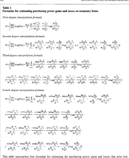
AND BUSINESS RESEARCH Table 1

Formulae for estimating purchasing power gains and losses on monetary items

zyxwvutsrqponmlkjihgfedcbaZYXWVUTSRQPONMLKJIHGFEDCBA

First-degree interpolation formula

Second-degree interpolation formula

Fourth-degree interpolation formula

2 7 7 m ( Y ) 6 4 0 m ( y ) 1 3 0 8 m ( Y ) 1472m( 4i-]

12 ) 527in(2) P(4i-])

1 4 j - 4 -

12

p( 12 ) 12 12

This table summarises four formulae for estimating the purchasing power gains and losses that arise over an annual period on an organisation’s monetary holdings. The formula in the first panel approximates the ratio

of the organisation’s monetary holdings to the price index,

zyxwvutsrqponmlkjihgfedcbaZYXWVUTSRQPONMLKJIHGFEDCBA

g,

and the logarithm of the price index, log[P(t)], by linear (or first-degree) interpolating polynomials. The formula in the second panel approximates and

log[P(t)] by quadratic (or second-degree) interpolating polynomials. The third panel is based on cubic (third degree) polynomial approximations while the fourth panel employs quartic (fourth-degree) polynomial approximations.

[image:5.540.55.483.81.605.2]

(6)

Vol. 37 No. 2.2007

small number of points at which the exact values of these functions are known. The case for this particular approximating procedure is strong (Carnahan et al., 1969:2-3). For a start, the theory of polynomial approximations is well developed and fairly simple. Furthermore, most of the other functions that one might consider as potential can- didates for approximation purposes (trigonomet- ric, logarithmic, exponential functions, etc.) must themselves be evaluated using these polynomial approximation techniques. Finally, there are strong analytical reasons for believing that interpolating polynomials will provide ‘good’ approximations to the real monetary holdings and price index functions. Here, ‘good’ implies that the differences between the approximating polynomial and the function being approximated can be reduced to an arbitrarily small figure. The important result here is the Weierstrass Approximation Theorem, which under a minimal set of regularity conditions and in the present context, says that the real monetary holdings and price index functions can be approximated to any desired degree of accuracy by a particular interpolating polynomial (Carnahan et al., 1969:3). Moreover, this result is normally implemented by employing low order interpolating polynomial approximation formulae (Carnahan et al., 1969:77). Given this, in Table 1 we summarise some low order approximating formulae for the purchasing power gain or loss based on the assumption that both the price index and real monetary holdings are observed on a monthly basis throughout the reporting year.

The formula in the first panel of this table

approximates

zyxwvutsrqponmlkjihgfedcbaZYXWVUTSRQPONMLKJIHGFEDCBA

%

and log[P(t)] by linear (or first

101

MI is the monetary aggregate which is normally employed in empirical work of the kind undertaken here. See. for example, Lucas (2000:248-252).

Simple algebraic manipulation shows that this formula

may be re-stated

as

This shows that the loss in purchasing power is comprised of the rate of inflation over the entire year multiplied by the currency on issue at the beginning of the year plus the rate of inflation over the period from time c until the end of the year multiplied by the change in the currency on issue during the year. Moreover, one can take the derivative through this ex- pression with respect to P(c) and thereby show:

Now, in hyperinflationary economies the currency on issue at the end of any period [m( I )] invariably exceeds the currency on issue at the beginning of the period [m(O)] by a consid- erable margin in which case the above derivative is negative. Minimal regularity conditions will then imply that the loss (or gain) in purchasing power on an organisation’s monetary items will decline as c + I .

degree) interpolating polynomials. The formula in the second panel approximates

%

and log[P(t)] by quadratic (or second degree) interpolating polynomials. The third panel is based on cubic (third degree) polynomial approximations whilst the fourth panel employs quartic (fourth degree) polynomial approximations. The Appendix provides further details about how these polynomial approximating formulae are determined.

One can demonstrate the application of these formulae by using them to estimate the loss in pur- chasing power for the currency on issue in the US and the UK. For the US the monetary aggregate

M 1 (currency, traveller’s checks, demand deposits and other checkable deposits) is taken to be the currency on issue whilst the inflation rate over any given period is determined from the Consumer Price Index (CPI)? The M 1 data were downloaded from the Federal Reserve Statistical Release website, http://www.federalreserve.gov/releases/h6/ hist/h6hist 1 .pdf, while CPI data were downloaded from the Economagic website, http://www.econo- m a g i c . c o m / e m - c g i / d a t a . e x e / b l s c u / CUUROOOOAAO. The results from applying the approximating formulae to these data are summarised in Table 2. The first column in this Table gives the year of the estimate while the next four columns contain the estimate of the loss in purchasing power on the currency using first, second, third and fourth-degree interpolating polynomial approximation. Thus, for the year ending 31 December 2005 the first, third and fourth-degree interpolation formulae estimate the purchasing power loss on the currency at $46.21 bn while the third-degree formula returns a marginally higher estimate of $46.23 bn. The final column of Table 2 contains the estimated loss in purchasing power computed by applying the procedures summarised in IAS 29. This procedure is based on para. 27 of IAS 29 and applies the appropriate rate of inflation to the currency on issue at the beginning and end of each year in accordance with the following formula:

I

0

zyxwvutsrqponmlkjihgfedcbaZYXWVUTSRQPONMLKJIHGFEDCBA

0

c

where c is some generally unknown number that lies between zero and one? This result is otherwise known as the (Weighted) Mean-Value Theorem for integrals (Apostol,l967: 219-220) and will always

(7)

102 ACCOUNTING

zyxwvutsrqponmlkjihgfedcbaZYXWVUTSRQPONMLKJIHGFEDCBA

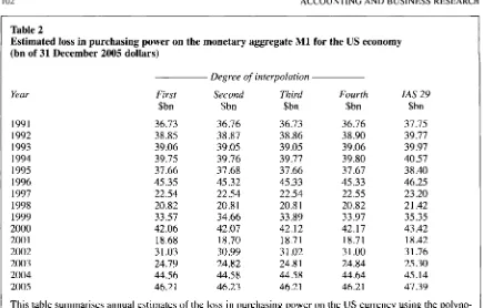
AND BUSINESS RESEARCH

Table 2

Estimated loss in purchasing power on the monetary aggregate M1 for the US economy

(bn of 31 December 2005 dollars)

zyxwvutsrqponmlkjihgfedcbaZYXWVUTSRQPONMLKJIHGFEDCBA

Year

1991 1992 1993 1994 1995 1996 1997 1998 1999 2000

200 1

2002

2003 2004 2005

Degree of interpolation

First Second Third Fourth IAS

zyxwvutsrqponmlkjihgfedcbaZYXWVUTSRQPONMLKJIHGFEDCBA

29

$bn $bn $bn $bn $bn

36.73 38.85 39.06 39.75 37.66 45.35 22.54 20.82 33.57 42.06 18.68

3 I .03 24.79 44.56 46.21 36.76 38.87 39.05 39.76 37.68 45.32 22.54 20.8 1 34.66 42.07 18.70 30.99 24.82 44.58 46.23 36.73 38.86 39.05 39.77 37.66 45.33 22.54 20.81 33.89 42.12 18.71

3 1.02 24.8 1 44.5 8 46.21 36.76 38.90 39.06 39.80 37.67 45.33 22.55 20.82 33.97 42.17 18.71

3 1 .OO

24.84 44.64 46.21 37.75 39.77 39.97 40.57 38.40 46.25 23.20 21.42 35.35 43.42 18.42 3 1.76 25.30 45.14 47.39

This table summarises annual estimates of the loss in purchasing power on the US currency using the polynomial formulae details of which are to be found in Table I . The column headed ‘first’ estimates the purchasing power loss using the first-degree (linear) interpolation formula; the column headed ‘second’ estimates the purchasing power loss using the second-degree (quadratic) interpolation formula; the column headed ‘third’ estimates the purchasing power loss using the cubic interpolation formula; the column headed ‘fourth’ estimates the purchasing power loss using quartic interpolation. The column headed ‘IAS 29’ estimates the purchasing power loss using the procedures endorsed by IAS 29: Financial Reporting in Hyperinflationary Economies.

Data for the monetary aggregate, M I , were downloaded from the Federal Reserve Statistical Release website,

http://www.federalreserve.gov/releases/h6/hist/h6hist1 .pdf, while Consumer Price Index data were downloaded from the Economagic website, http://www.economagic.com/em-cgi/data.exe/blscu/CUUROOOOAAO.

give the exact figure for the loss (or gain) in purchasing power on an organisation’s monetary holdings provided one is able to specify the “cor- rect” value of the parameter c. Unfortunately, there is no obvious way of either knowing or determin-

See the ‘illustrative example’ appended to IPSAS 10:

Finuncial Reporting in Hjperinjotionary Economies and AASB

129: Finunciul Reporting in Hvperinjlationury Econornies referred to earlier. Earlier examples of this convention are provided by para. 232 of the now withdrawn US Financial Accounting

Standards Board Statement #33: Financial Reporting

zyxwvutsrqponmlkjihgfedcbaZYXWVUTSRQPONMLKJIHGFEDCBA

of

Changing

zyxwvutsrqponmlkjihgfedcbaZYXWVUTSRQPONMLKJIHGFEDCBA

Prices and the illustrative example provided in the

Guidance Notes which accompany the (also withdrawn) U.K.

Accounting Standards Committee’s SSAP

zyxwvutsrqponmlkjihgfedcbaZYXWVUTSRQPONMLKJIHGFEDCBA

# 16: Ciirrerit Cost Accoimting. However, it is not hard to contemplate situations in

which this convention will lead to extremely poor estimates of purchasing power gains and losses. If an organisation operates under seasonal conditions - an ice-cream vendor, for example -

then its monetary position at the height of the season (m(+))may bear little resemblance to its monetary position at the beginning (m(O)) and end of the season (m(l)). If, for example, the ice- cream vendor carries no monetary items out of season so that m(O)=m( I )=0 then the above formula estimates the purchasing power gain on his monetary items at nothing. However, since at the height of summer the ice-cream vendor has borrowed heav- ily to finance his trading activities, the purchasing power gain on his debt will be significant.

ing c in any specific inflationary environment and given this, a convention has arisen which lets c

=+8

Note that under this convention Table 2 shows that the IAS 29 procedures return an estimated purchasing power loss for the year ending 31 December 2005, which is over $Ibn higher than the estimated purchasing power losses under the polynomial formulae. Against this, the four polynomial approximation methods return almost identical estimates of the loss in purchasing power in

any given year. Moreover, the IAS 29 procedures return estimates of the loss in purchasing power which, in all but one year (2001) are larger than those obtained from the four polynomial interpolation methods.

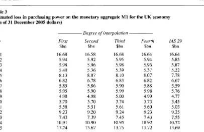
Table 3 summarises similar information relating

to the loss in purchasing power on the U.K. currency. Again, the monetary aggregate M1 is taken to be the currency on issue and data for this variable were downloaded from the Bank of England website. Data for the UK Consumer Price index were downloaded from the UK National Statistics Office website. The results from applying the approximating formulae to the UK data are sum- marised in Table 3 . The format of this table is the

[image:7.540.54.489.77.355.2]

(8)

[image:8.540.75.481.85.349.2]

Vol.

zyxwvutsrqponmlkjihgfedcbaZYXWVUTSRQPONMLKJIHGFEDCBA

37 No. 2.2007 103

Table 3

Estimated loss in purchasing power on the monetary aggregate M1 for the UK economy

(Ebn of 31 December 2005 dollars)

zyxwvutsrqponmlkjihgfedcbaZYXWVUTSRQPONMLKJIHGFEDCBA

Year 1991 1992 1993 1994 1995 1996 1997 1998 1999 2000 200 1 2002 2003 2004 2005

Degree of interpolation

First Second Third Fourth

IAS 29

$bn $bn $bn $bn $bn 16.68 5.94 5.98 5.40 8.13 6.82 5.85 5.95 4.98 3.70 5.58 9.23 7.43 10.91 13.74 16.58 5.92 5.96 5.36 8.07 6.78 5.86 5.90 4.98 3.70 5.51 9.20 7.39 10.90 13.67 16.68 5.95 5.98 5.39 8.10 6.83 5.90 5.99 5 .00 3.74 5.61 9.24 7.45 10.95 13.75 16.64 5.94 5.96 5.37 8.07 6.82 5.88 5.98 4.99 3.73 5.60 9.23 7.43 10.92 13.72 16.64 5.85 5.87 5.22 7.78 6.67 5.59 5.76 4.77 3.45 5.03 9.25 7.55 10.72 13.69

This table summarises annual estimates of the loss in purchasing power on the UK currency using the polyno-

mial formulae, details of which are to be found in Table

1. The column headed ‘first’ estimates the purchasing power loss using the first-degree (linear) interpolation formula; the column headed ‘second’ estimates the pur-

chasing power loss using the second-degree (quadratic) interpolation formula; the column headed ‘third’ estimates the purchasing power loss using the cubic interpolation formula; the column headed ‘fourth’ estimates the purchasing power loss using quartic interpolation. The column headed ‘IAS 29’ estimates the purchasing

power loss using the procedures endorsed by IAS 29: Financial Reporting in Hyperinflationary Economies. Data for the monetary aggregate, M1, were downloaded from the Bank of England website while Consumer Price Index data were downloaded from the UK National Statistics Office website.

same as that for Table 2. Note how this table again shows that the four polynomial interpolation methods return almost identical estimates of the loss in purchasing power on the currency. However, when the IAS 29 procedures are applied to the UK data they return a lower estimate of the loss in purchas-

ing power on the currency than is the case with the polynomial approximation methods in all but two years (2002 and 2003). This is in direct contrast to the US results, where the IAS 29 procedures con- sistently return higher estimates of the loss in purchasing power on the currency.

One might argue that the systematic differences observed in these two tables are of little consequence since the deviations between the annual estimates obtained under the IAS 29 procedures and the polynomial approximation techniques are relatively small. For the US data, estimates obtained using the polynomial approximation formulae

vary by no more than 4% from estimates obtained under the IAS 29 procedures. For the UK data, there are two years (2000 and 2001) where differences in the estimates are in excess of 8%. In other years, however, the differences are generally much less than 5 % . Here, one must remember however that these differences have arisen in what can only

be described as modest inflationary environments. The average annual rate of inflation over the 15- year period ending 31 December 2005 was 2.6% for the US and a mere 2.1% for the UK. However, in the hyperinflationary environments envisaged by IAS 29 the cumulative rate of inflation over the previous three years will typically be of the order of 100% or more. It is questionable whether results obtained for the relatively low inflationary environments experienced in the US and UK can be replicated in the hyperinflationary environments envisaged by IAS 29. Given this, in the next sec-

tion we use the data pertaining to 32 hyperinflationary economies and which between them encompass a wide variety of hyperinflationary environments covering a period of over eighty years, to make assessments about the relative efficiency of the procedures summarised in IAS 29 for estimating purchasing power gains and losses during hyperinflationary periods.

3. Data and empirical analysis

Our empirical analysis is based on the seven hyperinflations analysed by Cagan (1956) as well as a further 25 hyperinflationary economies for

(9)

I04

ACCOUNTING AND BUSINESS RESEARCH

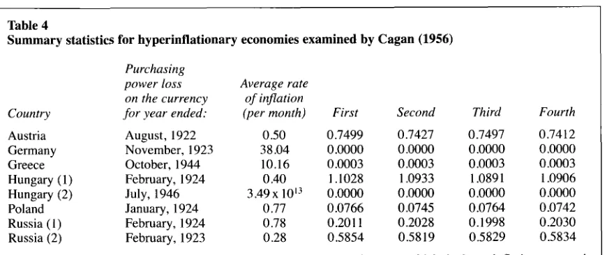
Table 4

Summary statistics for hyperinflationary economies examined by Cagan (1956)

zyxwvutsrqponmlkjihgfedcbaZYXWVUTSRQPONMLKJIHGFEDCBA

Purchasing

power loss Average rate on the currency of inflation

Country f o r year ended: (per month) First Second Third Fourth Austria

Germany Greece Hungary (1)

Hungary (2)

Poland

Russia

(1) Russia (2)

August, 1922 0 S O

November, 1923 38.04

October, 1944 10.16

February, 1924 0.40

January, 1924 0.77

February, 1924 0.78

February, 1923 0.28

July, 1946 3.49x 1 0 ’ 3

0.7499 0.0000 0.0003 1.1028 0

.oooo

0.0766 0.201 1 0.5854

0.7427 0

.oooo

0.0003 1.0933 0

.oooo

0.0745 0.2028 0.5819

0.7497 0

.oooo

0.0003 1.089 1 0

.oooo

0.0764 0.1998 0.5829

0.7412 0

.oooo

0.0003 1.0906 0

.oooo

0.0742 0.2030 0.5834

The first and second columns in this table give the country and period over which the hyperinflation occurred. The third column summarises the average monthly rate of inflation over the duration of the given hyperinflation. Thus, the average rate of inflation for the Austrian economy in the year to August 1922 amounts to 50%

(per month). Likewise, the average rate of inflation for the Polish economy in the year to January 1924 amounts to 77% (per month). The column headed ‘first’ gives the ratio of the estimated purchasing power loss based on

the linear interpolation formula summarised in Table 1 to the estimate obtained using the IAS 29 procedures; the column headed ‘second’ gives the ratio of the estimated purchasing power loss based on the quadratic interpolation formula summarised in Table 1 to the estimate obtained using the IAS 29 procedures; the column headed ‘third’ gives the ratio of the estimated purchasing power loss based on cubic interpolation to the estimate obtained using the IAS 29 procedures; the column headed ‘fourth’ gives the ratio of the estimated purchasing power loss based on quartic interpolation to the estimate obtained using the IAS 29 procedures. The

data on which this table is based are taken from Cagan (1956).

which data are available from the International Monetary Fund’s website. Summary details of the hyperinflationary economies analysed by Cagan (1956) are contained in Table 4. Cagan (1 956:26) shows that the first of these hyperinflations - namely, the Austrian hyperinflation - lasted for about a year and petered out towards the end of August 1922. The average rate of inflation over the year ending on this date was 50% (per month). The final four columns give the ratio of the estimated loss in purchasing power on the Austrian currency for the year ending August 1922 from applying the polynomial approximating formulae, to the estimated loss in purchasing power from applying the IAS 29 procedures. These ratios are all in the vicinity of 0.75, which implies that the estimates of the purchasing power loss using the polynomial approximating formulae are approximately 25% lower than the estimates obtained from using the IAS 29 procedures. Against this, Table 4 shows that the estimates of the loss in purchasing power on the Hungarian currency for the year ending February 1924 using the polynomial approximating formulae are about 9% larger than the estimated loss in purchasing power obtained from the IAS 29 procedures. With the exception of Russia, the

The other six hyperinflations summarised in Table 4 all lasted for around a year or less.

other statistics summarised in Table 4 are to be interpreted in the same way as those for the Austrian and Hungarian hyperinflations. The Russian hyperinflation began in December 192 1 and concluded approximately 26 months later in February 1924.9 Given this, one can estimate the loss in purchasing power from holding the Russian currency for two annual periods. The first of these is for the year ending February 1923 for which the estimated losses in purchasing power under the polynomial approximating formulae are about 40% lower than the estimated purchasing power losses computed under the IAS 29 procedures. For the second of these periods - the year ending February 1924 -

the estimated losses in purchasing power under the polynomial approximating formulae are about 80% lower than the estimated losses obtained from the IAS 29 procedures.

Overall, Table 4 shows that the IAS 29 procedures tend to return significantly larger estimates of the loss in purchasing power when compared with the polynomial approximating formulae. In six of the seven hyperinflations examined by Cagan (1956), Table 4 shows that the estimated loss in purchasing power on the currency is significantly lower under the polynomial approximating formulae than is the case with IAS 29 procedures. Indeed, for the German hyperinflation the polynomial estimate of the purchasing power loss on the currency is on average barely 0.000016% of the

[image:9.540.54.489.88.271.2]

(10)

Vol. 37 No. 2.2007

estimate obtained from the IAS 29 procedures whilst for the Hungarian hyperinflation which concluded in July 1946, the polynomial estimate is

on average just 4.33xlO-*O% of the estimate obtained from the IAS 29 procedures. The root cause of these gigantic differences appears to lie in the fact that with the exception of the Greek hyperinflation, the inflation rate for each country accelerates towards the end of the hyperinflationary period and the real currency on issue declines instantaneously and dramatically in response to it. In other words, organisations adjust their monetary holdings in response to changes in the inflation rate much more frequently than the once or twice a year scenario envisaged by the IAS 29 proce-

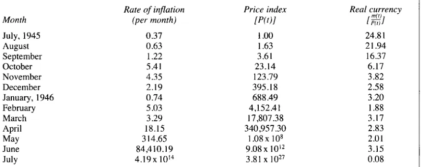
dures. One can see this more clearly from Table

zyxwvutsrqponmlkjihgfedcbaZYXWVUTSRQPONMLKJIHGFEDCBA

5 , which summarises an index of the real currency on

issue during each month as well as the monthly rate of inflation and the price index for the Hungarian hyperinflation, which endured over the year to July, 1946 (Cagan, 1956: 110-111). Note how this table shows that by October 1945, the

real value of the currency on issue was just a fourth of what it had been in July 1945 and that by January 1946, it was an eighth of what it had been

just six months' earlier. In other words, when the

105

inflation rate is rapidly increasing organisations adjust their monetary holdings much more frequently than the one or two occasions envisaged by the IAS 29 procedures and so, they will more than likely return unreliable estimates of purchasing power losses as a consequence. The polynomial interpolating techniques, however, are based on the assumption that the real value of the currency on issue changes instantaneously in response to variations in the rate of inflation and therefore, they are unlikely to suffer from this problem. Given this, one should not be too surprised to see the large differences in the estimated purchasing power losses that are summarised in Table 4.1°

Table 6 provides summary information relating to the 25 more recent hyperinflationary economies for which data are available from the International Monetary Fund's (IMF) website, http://www.imfstatistics.org/imf/. As with our estimates of the pur-

chasing power losses for the UK and

zyxwvutsrqponmlkjihgfedcbaZYXWVUTSRQPONMLKJIHGFEDCBA

US, we take

M1 to be the currency on issue (Lucas, 2000:

248-252) while the inflation rate over any given period is determined from the Consumer Price Index (CPI) for the particular country. The first two columns in Table 6 give the country and the period over which the hyperinflation was deemed

lo Using the polynomial formulae summarised in Table 1

shows that our best estimate of the loss in purchasing power on the Hungarian currency for the year to July 1946 amounts to

]g.dlog[P(f)l = 185.45

zyxwvutsrqponmlkjihgfedcbaZYXWVUTSRQPONMLKJIHGFEDCBA

0

where the loss in purchasing power is stated in units of July 1946 purchasing power. Now, the weighted mean value theorem given earlier shows that the purchasing power loss has the following representation over this period:

where c is some generally unknown parameter that lies between zero and unity. This means that if one follows the usual

convention of letting c =

4

zyxwvutsrqponmlkjihgfedcbaZYXWVUTSRQPONMLKJIHGFEDCBA

one obtains the following estimate of the purchasing power loss for the Hungarian hyperinflation

under the IAS 29 procedures:

68849 i

+ l , ~ 8 x 7 ~ ~ ~ ~ u 2 7 . ~ ~ n 4 ~ 2 4 8 1 x 68x49

688 49

o r 2 4 . 7 7 + 4 . 2 9 ~ 1 0 ~ ~ = 4 . 2 9 ~ 1 0 ~ ~ in units of July 1946 purchasing power. From this it follows that the ratio of our best estimate of the purchasing power loss to the estimate of the purchasing power loss under the I A S 29 procedures is as stated in the text. Here, however, Table 5 shows that the average monthly rate of inflation for the six months ending in

July, 1946 is 6.98x1Ol3, a figure that far exceeds the rates of inflation for the months of February, March, April, May and June, 1946. This shows that the distribution of the monthly

rates of inflation is highly skewed and so a simple average of these rates of inflation provides a poor summary measure of the inflation rate over this period. Likewise, the inflation rate used to estimate purchasing power losses under IAS 29 over the six months ending in July, 1946 - namely.

- will also be a poor reflection of the rate of inflation over this period and will lead to the enormous errors documented for the Hungarian hyperinflation summarised in Table 4. We have previously shown, however, that one can address this problem by letting the unknown parameter c

+

1 . Given this one can base the estimate of the loss in purchasing power in the Hungarian currency on the price index at the beginning of August 1945 (time zero), the price index at the end of June, 1946 (thereby setting c =

fi)

and the price index at the end of July 1946 (time one). Using the data summarised in Table 5 we then have the following estimate of the purchasing power loss for the Hungarian hyperinflation:

o r 2 4 3 1 + 3 . 2 5 ~ 1 0 ~ ~ = 3 . 2 5 ~ 1 0 ' ~ in unitsofJuly, 1946purchas- ing power. While this estimate is about half the figure obtained under the IAS 29 procedures (where, it will be recalled c =+), it is still substantially larger than our best estimate of the purchasing power loss (185.45) given earlier. This reflects the fact that the rate of inflation for July 1946 is gigantic when compared to the rates of inflation for the other months in the year ending in July 1946. This in turn means that the parameter c will have to be very close to but not quite equal to unity if the weighted mean value formula is to give a reliable estimate of the purchasing power loss for the Hungarian hyperinflation.

(11)

106 ACCOUNTING

zyxwvutsrqponmlkjihgfedcbaZYXWVUTSRQPONMLKJIHGFEDCBA

AND BUSINESS RESEARCH Table 5

Monthly inflation rates and index of real currency on issue for Hungarian hyperinflation ending in

July 1946

zyxwvutsrqponmlkjihgfedcbaZYXWVUTSRQPONMLKJIHGFEDCBA

Month

July, 1945

August September October November December January, 1946

February March April June

July May

Rate

zyxwvutsrqponmlkjihgfedcbaZYXWVUTSRQPONMLKJIHGFEDCBA

of inflation Price index Real currency

(per month)

[P(t)I

#I

0.37 0.63 1.22 5.41 4.35 2.19 0.74 5.03 3.29 18.15 314.65 84,4 10.19

4 . 1 9 ~ 1014

1

.oo

1.63 3.61 23.14 123.79 395.18 688.49

4,152.4 1

17,807.38 340,957.30

1 . 0 8 ~ 10' 9.08 x 10I2 3.81 1027

24.8 1

21.94 16.37 6.17 3.82 2.58 3.20 1.88 3.17 2.83 2.01 3.15 0.08

The first column in the table gives the month and year of the Hungarian hyperinflation, which concluded in July 1946. The second column gives the rate of inflation during the given month. Thus, the rate of inflation for

the month of July, 1945 was 37% and the rate of inflation for the month of April 1946 was 13415%. The third column summarises the price index constructed from the inflation rates given in the second column. Thus, the

price index for the end of August 1945 is one plus the inflation rate during August 1945 or 1.63. The price index for September 1945 is one plus the inflation rate for September, 1945 multiplied by the price index for August,

1945 or 2.22 x 1.63 = 3.61. Likewise, the price index for October 1945 is one plus the inflation rate for October

1945 multiplied by the price index for September 1945 or 6.41 x 3.61 = 23.14. Finally, the last column is an

index of the real currency on issue during the given month. to have occurred. In conformity with para. 3 of IAS 29, a hyperinflationary period was deemed to commence at the beginning of any three-year period for which the accumulated rate of inflation ex- ceeded 100%. The hyperinflationary period was deemed to have concluded at the end of any three- year period for which the accumulated rate of inflation had fallen below 100%. Thus, under these criteria the Argentinean hyperinflation was deemed to have commenced at the beginning of 1971 and continued for 23 years before petering out at the end of 1993. The next four columns give the average annual rate of inflation, the standard deviation of the annual rate of inflation and the minimum and maximum annual rates of inflation over this 23-year hyperinflationary period. This shows that the average rate of inflation during the Argentinean hyperinflation was 447.68% (per annum); that the standard deviation of the annual rate of inflation rate was 996.22%; that the maximum rate of inflation during this period was 4,923.32% (per annum) whilst the minimum rate of inflation was 7.36% (per annum). The other statistics summarised in Table 6 are to be interpreted in the same way as those for the Argentinean hyperinflation. Here we also need to emphasise that the data for some countries are incomplete (e.g. Democratic Republic of Congo, Russia and Zimbabwe among

others) and that this placed limits on the extent to which the relevant hyperinflations could be analysed.

Table 7 summarises the relative loss in purchasing power on the currency on issue for each of the 25 hyperinflationary economies for which data are available from the IMF website under the four polynomial approximating techniques as compared to those obtained from the simple IAS 29 estimation procedures. The first two columns in this table identify the country and duration of the hyperinflation. The third column summarises the number of years over which our analysis is based. Hence, for Argentina our analysis covers the 23- year period from 1971 to 1993. The next two columns give the median of the ratio of the loss in purchasing power from using the polynomial approximating techniques to the loss in purchasing power as calculated from the IAS 29 procedures. Thus, for the Argentinean hyperinflation the 23 ra-

tios are ordered from smallest to largest for each of the four polynomial approximating techniques. The twelfth ordered ratio is the median and it is this statistic which is reported in Table 7 for each polynomial technique. Thus, these results show that for the Argentinean hyperinflation the median estimate of the purchasing power loss for the polynomial approximating techniques is about 10%

[image:11.540.56.492.99.311.2] [image:11.540.61.489.141.311.2]

(12)

Vol.

zyxwvutsrqponmlkjihgfedcbaZYXWVUTSRQPONMLKJIHGFEDCBA

37 No. 2. 2007 107

Table 6

Summary statistics for hyperinflationary economies with data available on the International Monetary

Fund (IMF) website: http://www.imfstatistics.org/imf/

zyxwvutsrqponmlkjihgfedcbaZYXWVUTSRQPONMLKJIHGFEDCBA

Country Angola Argentina Belarus Bolivia Brazil Chile Congo, De R. Dominican Re Ecuador Estonia Israel Jamaica Madagascar Mexico Nicaragua Peru Poland Romania Russia Suriname Turkey Ukraine Uruguay Venezuela Zimbabwe

Period of

hyperinflation 1996-2005 1995-2003 197 1-1993 1979-1988 1980-1 996 1968-1976 1976-1 995 1989-1 99 1

1984-2002 1993-1 995 1974-1987

199 1-

I994 1994-1 996 1986-1 990 1988-1993 1976- 1994 1990-1995 1994-2002 1992-2002 1977-2003 1993- I 997 1976-1 996 1987-1998

1998-200

1

1998-2000

Average rate

zyxwvutsrqponmlkjihgfedcbaZYXWVUTSRQPONMLKJIHGFEDCBA

of inflation (per annunz)

2.7065 4.4768

1 .I034 11.1654 6.4424

1.9008 11.5316 0.408 1

0.4054 0.3537

1 .lo32 0.4433 0.3560 0.7324 66.8353 7.0490 0.6995 4.1650 0.4704 1.0634 0.5912 21 S756 0.5866 0.5002 0.677 1

Standard deviation

of rate of inflation 4.6465 9.9622 0.8637 24.3383 7.3473 1.8264 24.2986 0.2973 0.2143 0.0643 1.1300 0.2129 0.2164 0.5225 90.8414 17.7508 0.7076 0.3723 0.2724 I .6377 0.2346 40.0113 0.2486 0.224 1 0.259 1

Maximum rate of inflation

16.501 1

49.23 32 2.5120 8 1.7052 24.7714 5.5862 97.9689 0.7992 0.9100 0.4165 4.4488 0.8019 0.6122 1.5916 240.3105 76.4975 2.2587 1.5142 0.8438 5.8648 1.2025 10 1.5503 1.2895 1.0324 1.1207 Minimum rate of inflation 0.1853 0.0736 0.2540 0.1066 0.0956 0.1940 0.1433 0.0790 0.0936 0.2653 0.1610 0.2679 0.0828 0.1970 0.0352 0.1538 0.2195 0.1784 0.2018 0.0122 0.1613 0.1012 0.2053 0.299 1 0.4663 The first and second columns in the table give the country and period over which the hyperinflation occurred. The third and fourth columns summarise the average annual rate of inflation and the standard deviation of the annual rate of inflation over the duration of the given hyperinflation. Thus, the average annual rate of inflation for the Mexican economy was 73.24% with a standard deviation of 52.25%. The fifth and sixth columns give the maximum and minimum annual rates of inflation over the period of the hyperinflation.

lower than the purchasing power loss computed under the IAS 29 procedures. Furthermore, one

can average the four polynomial estimates of the purchasing power loss and then divide this average

by the estimate of the purchasing power loss obtained from the IAS 29 procedures. The final two columns give the number of these (average) ratios that are less than one and the number that exceed

unity. Hence, for the 23 years on which our analy-

sis of the Argentinean hyperinflation is based,

there are 20 years in which this (average) ratio is less than one and only three years in which the (average) ratio exceeds one. The other statistics sum- marked in Table 7 are to be interpreted in the same

way as those for the Argentinean hyperinflation. Probably the most striking characteristic displayed by Table 7 is that for all but one country (namely, Belarus), the median ratios are less than

unity. Indeed, of the 272 country-years on which

Table 7 is based, there are 229 occasions on which the ratio of the estimated purchasing power loss from the polynomial approximating formulae to the estimated loss under the IAS 29 procedures is less than unity, and only 43 occasions where the ratio exceeds unity. Moreover, a simple sign test rejects the null hypothesis that the median ratio for the ‘population’ of hyperinflationary economies is equal to unity at any reasonable level of signifi- cance [Conover (1971:121-126)]. This, of course, is compatible with the hypothesis that the polynomial-based formulae will tend to return lower estimates of purchasing power losses than will be the case with the IAS 29 procedures.

Here it is important to note, however, that for the more recent hyperinflationary economies extracted from the IMF website, the differences between the polynomial-based approximations of the purchasing power loss and those based on the IAS 29

[image:12.540.62.482.112.454.2]

(13)

Table 7

Median ratio of the average of four polynomial estimates to the IAS 29 estimate of the annual purchasing power loss for hyperinflationary economies with

data available on the International Monetary Fund (IMF) website: http:Nwww.imfstatistics.org/imf/

zyxwvutsrqponmlkjihgfedcbaZYXWVUTSRQPONMLKJIHGFEDCBA

Country Period o j hyperinflation

# Observations

Argentina 197 1-1993 23

Belarus 1995-2003 9

Bolivia 1979-1988 10

Brazil 1980-1996 17

Chile 1968-1 976 9

Dominican Re 1 989-1 99 1 3

Ecuador 1984-2002 19

Estonia 1993-1995 3

Israel 1974-1987 14

Jamaica 1991-1994 4

Mexico 1986-1990 5

Nicaragua 1988-1993 6

Peru 1976-1 994 19

Poland 1990- 1995 6

Romania 1994-2002 9

Russia 1998-2000 3

Suriname 1992-2002 11

Turkey 1977-2003 27

Ukraine 1993-1 997 5

Venezuela 1987- 1998 12

Zimbabwe 1998-2001 4

TOTALS 272

Angola 1996-2005 I0

Congo, De R. 1976-1995 20

Madagascar 1994- 1996 3

Uruguay 1976-1 996 21

First 0.8210 0.8909 1.0239 0.8647 0.8183 0.9770 0.9430 0.8807 0.9190 0.9556 0.9719 0.953 1 0.9719 0.8494 0.9730 0.9174 0.9489 0.8427 0.9383 0.9797 0.8050 0.9478 0.8833 0.9028 0.9865 Second 0.8161 0.902 1 1.022 1

0.8652 0.8 139 0.9834 0.9445 0.8788 0.9133 0.9555 0.9740 0.9487 0.9743 0.8461 0.9661 0.9175 0.9467 0.8392 0.9365 0.9754 0.7984 0.944 1

0.8773 0.9014 0.9855 Third 0.8135 0.8975 1.0217 0.8647 0.8077 0.9752 0.9403 0.8790 0.9155 0.9553 0.9655 0.9486 0.9724 0.8477 0.9677 0.9177 0.9485 0.8397 0.9364 0.9808 0.8028 0.9428 0.8814 0.8977 0.9859 Fourth 0.8147 0.9035 1.0225 0.8667 0.8122 0.9853 0.9428 0.878 1 0.9117 0.9567 0.9755 0.9468 0.9769 0.8455 0.9602 0.9181 0.9466 0.8394 0.9369 0.9759 0.7958 0.9428 0.8779 0.90 12 0.9843

Ratios < 1 9 20 3 9 15 6 13 3 16 3 9 3 3 5 4 19 4 9 3 8 27 4 21 11 2 229

Ratios > I

1 3 6 1 2 3 7 0 3 0 5 1 0 0 2 0

2

zyxwvutsrqponmlkjihgfedcbaZYXWVUTSRQPONMLKJIHGFEDCBA

0 0 3

0

1

0

1 2 43

The first, second and third columns in the table give the country, the period and the number of years over which the hyperinflation occurred. The column headed ‘first’ gives the median ratio of the estimated purchasing power loss based on the linear interpolation formula summarised in Table 1 to the estimate obtained using the IAS 29 procedures; the column headed ‘second‘ gives the median ratio of the estimated purchasing power loss based on the quadratic interpolation formula summarised in Table 1 to the estimate obtained using the IAS 29 procedures; the column headed ‘third’ gives the median ratio of the estimated purchasing power loss based on cubic

interpolation to the estimate obtained using the IAS 29 procedures; the column headed ‘fourth’ gives the median ratio of the estimated purchasing power loss based on cubic interpolation to the estimate obtained using the IAS 29 procedures. The penultimate column gives the number of observations for which the simple average of the first, second, third and fourth interpolating ratios for each year is less than unity. The final column gives the number of observations for which the simple average of the first, second, third and fourth interpolating ratios for each year exceeds unity.

[image:13.540.78.742.88.392.2]

(14)

[image:14.540.55.485.77.335.2]

Vol. 37 No.

zyxwvutsrqponmlkjihgfedcbaZYXWVUTSRQPONMLKJIHGFEDCBA

2.2007

109

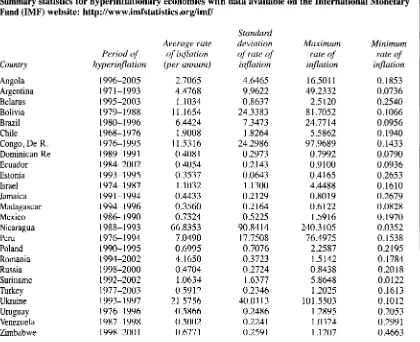
Figure 1

Index of real currency on issue and monthly rate of inflation for Argentinean economy from January

1971 (month 1) until December 1993 (month 276)

zyxwvutsrqponmlkjihgfedcbaZYXWVUTSRQPONMLKJIHGFEDCBA

0.25

a

IL 0.20

o w

Z Z

W

IY

0.15

0 0

f

&

0.10 W Z I - W

2 5

0.05

Z 3

Q"

2

0.00

z

-I IL

-0.05

21 41 61 81 101 121 141 161 181 201 221 241 261

MONTH OF HYPERINFLATION

The data series that starts at just above 0.15 at month zero and then gradually declines is an index of the real currency on issue. The data series that begins at just above the origin at time zero and then gradually increases is the continuously compounded monthly rate of inflation divided by 5. The currency on issue series was extracted from line 34 of the International Monetary Fund's database, http://www.imfstatistics.org/imf/. The

[image:14.540.53.486.347.665.2]

Consumer Price Index series was extracted from line 64 of the IMF's database.

Figure 2

Index of real currency on issue and monthly rate of inflation for Israeli economy from January 1974 (month 1) until December 1987 (month 168)

0.4 1 I

13 25 37 49 61 73 85 97 I09121 133145157

MONTH OF HYPERINFLATION

-0.05

The data series that starts at just above 0.35 at month zero and then gradually declines is an index of the real currency on issue. The data series that begins at just below 0.05 at time zero and then gradually increases is the continuously compounded monthly rate of inflation. The currency on issue series was extracted from line 34 of the International Monetary Fund's database, http:Nwww.imfstatistics.org/imf/. The Consumer Price Index series was extracted from line 64 of the IMF's database.

(15)

[image:15.540.54.487.90.332.2]

I10 ACCOUNTING AND BUSINESS RESEARCH

zyxwvutsrqponmlkjihgfedcbaZYXWVUTSRQPONMLKJIHGFEDCBA

Figure 3

Index of real currency on issue and monthly rate of inflation for Peruvian economy from January 1976

(month until December 1994 (month 228)

zyxwvutsrqponmlkjihgfedcbaZYXWVUTSRQPONMLKJIHGFEDCBA

0.90

w 0.80

(2:

0 0.70

X X

$

0.60

z z

0 0 0 5 0

= t

p

0.40

I - w

$ 5

030

2 3

d

LL

0

*

0.20

2

0.10

z

0.00

1 17 33 49 65 81 97 1 1 3 1 2 9 1 4 5 1 6 1 1 7 7 1 9 3 2 0 9 2 2 !

MONTH OF HYPERINFLATION

[image:15.540.54.490.364.667.2]

The data series that starts at just below 0.50 at month zero and then gradually declines is an index of the real currency on issue. The data series that begins just above the origin at time zero and then gradually increases is the continuously compounded monthly rate of inflation divided by two. The currency on issue series was extracted from line 34 of the International Monetary Fund's database, http://www.imfstatistics.org/imf/. The Consumer Price Index series was extracted from line 64 of the IMF's database.

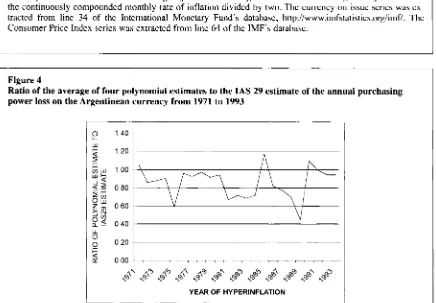
Figure 4

Ratio of the average of four polynomial estimates to the IAS 29 estimate of the annual purchasing power loss on the Argentinean currency from 1971 to 1993

p

1.40

W

k

1.20 0.20

I-

Q

D! 0.00

B

0

\

n

L

9

/---I

I \

1 -

\I

L-'

\ i

zyxwvutsrqponmlkjihgfedcbaZYXWVUTSRQPONMLKJIHGFEDCBA

V

YEA!? OF HYPERINFLATION

~ ~- ~~~ ~

This graph depicts the ratio of two data series. The first is based on the four estimates of the purchasing power loss on the Argentinean currency using the polynomial formulae summarised in Table I . For each year, the four estimates obtained from these formulae are averaged to give the first data series. The second data series esti- mates the purchasing power loss using the IAS 29 procedures. The graph summarises the ratio of the average polynomial estimate to the IAS 29 estimate of the purchasing power loss for each year of the Argentinean hyperinflation.

(16)

Vol. 37 No.

zyxwvutsrqponmlkjihgfedcbaZYXWVUTSRQPONMLKJIHGFEDCBA

2. 2007

procedures are much smaller than is the case for the earlier hyper-inflations examined by Cagan (1956).” We have previously noted that the princi-

pal reason for this is that the hyperinflations examined by Cagan (1956) were characterised by rapidly increasing rates of inflation that reached a crescendo over a short period of time (typically one to two years or less) and then quickly petered out. Moreover, during this period of rapidly increasing inflation there is a precipitous decline in the real value of the currency on issue. The more recent IMF hyperinflations in contrast have tended

to be of much longer duration (typically five to 20 years) and the real value of the currency on issue has tended to decline much more slowly for the IMF hyperinflations than is the case with the

Cagan

zyxwvutsrqponmlkjihgfedcbaZYXWVUTSRQPONMLKJIHGFEDCBA

( 1956) hyperinflations. This is illustrated by Figures 1 , 2 and

3 , which graph the time series

of an index of the real currency on issue and the monthly rate of inflation for the Argentinean, Israeli and Peruvian hyperinflations, respectively. These graphs, which are typical of the 25 hyperinflations for which data are available from the IMF web site show that the rate of decline in the index

of real currency on issue is quite modest when compared to the ‘equivalent’ data for the Hungarian hyperinflation of 1945 and 1946 examined by Cagan (1956), details of which are sum-

marised in Table

zyxwvutsrqponmlkjihgfedcbaZYXWVUTSRQPONMLKJIHGFEDCBA

5 . This means that for the IMF hyperinflations the beginning of the year and end

of year figures for the real value currency on issue (and their associated inflation rates) are much more likely to be ‘representative’ of their values over the entire year than will be the will be the case for the Cagan (1956) hyperinflations. Hence, it is more likely that the IAS 29 procedures, which are based on just these two observations of the real value of the currency on issue (and their associated inflation rates), will provide more reliable estimates of the purchasing power losses from inflation than is the case when it is applied to the ‘short, sharp’ hyperinflations examined by Cagan (1956). Against this, it must be emphasised that even for the IMF hyperinflations summarised in Table 7 the IAS 29 procedures appear to return estimated purchasing power losses that typically, are 10% higher than those obtained from using the four polynomial approximation formulae summarised in Table 1 .

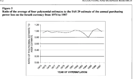
However, even for the IMF hyperinflations there is a great deal of variation in the data. For the

1 I 1

~

” Except for the Hungarian hyperinflation, which petered

out in February 1924, Table 4

zyxwvutsrqponmlkjihgfedcbaZYXWVUTSRQPONMLKJIHGFEDCBA

shows that the median ratios for the polynomial approximations to the estimates obtained from

the IAS 29 procedures are all less than 0.75. While Table 7 shows that with one exception (Belarus) the equivalent ratios for the post-war hyperinflations are all less than unity, they are nonetheless much higher than the 0.75 recorded for the ‘high- est’ median ratio for the Cagan (1956) hyperinflations.

Argentinean hyperinflation, the ratio of the average of the four polynomial estimates of the purchasing power loss to the purchasing power loss

obtained from the IAS 29 procedures varies from 0.4469 in 1989 to 1.1744 in 1985. The complete time series of this ratio for the Argentinean hyperinflation is displayed in Figure 4. Likewise, for the Israeli hyperinflation this ratio varies from 0.7954 in 1984 to 1.0754 in 1986. Again, the complete time series of this ratio for the Israeli economy is displayed in Figure 5 . Finally, for the Peruvian hyperinflation, the ratio of the average of the four polynomial estimates of the purchasing power loss to the purchasing power loss obtained from the IAS 29 procedures varies from 0.2592 in 1990 to 0.9962 in 1994. The complete time series of this ratio for the Peruvian economy is displayed in