New York J. Math. 17a(2011) 127–146.
On the computation of the Fourier
transform under the presence of nearby
polar singularities
Ruym´
an Cruz-Barroso, Pablo Gonz´
alez-Vera
and Francisco Perdomo-P´ıo
Abstract. In this paper we present a procedure for the computation of integrals on the whole real line with nearby singularities. The method is based in collecting the possible singularities of the integrand within a weight function on the real line, passing to the unit circle by considering an associated weight function there and then making use of Szeg˝o or interpolatory-type quadrature formulas. This algorithm is applied in order to provide a computational method for the Fourier transform of a function exhibiting polar singularities near the range of integration. Some error bounds for the estimations are presented and some numerical experiments carried out.
Contents
1. Introduction 128
2. Quadrature formulas on the unit circle 129
3. Computation of integrals on the whole real line with nearby
singularities 133
4. An application to the Fourier transform 137
5. Numerical examples 142
References 144
Received August 13, 2010.
2000Mathematics Subject Classification. 41A55, 42C05, 65D30, 42A38.
Key words and phrases. Fourier transform, Szeg˝o quadrature formulas, interpolatory-type quadrature formulas, error bounds.
This work is partially supported by Direcci´on General de Programas y Transferencia de Conocimiento, Ministerio de Ciencia e Innovaci´on of Spain under grant MTM 2008-06671. The work of the third author has been partially supported also by a Grant of Agen-cia Canaria de Investigaci´on, Innovaci´on y Sociedad de la Informaci´on del Gobierno de Canarias.
ISSN 1076-9803/2011
1. Introduction
Given a pair of functions related by the expression
(1) G(w) =
Z b
a
g(t)K(w, t)dt,
we say thatG(w) is the integral transform ofg(t) andK(w, t) its kernel. As it is known, the computation of the integral (1) is often a difficult task because of the possible infinite range of integration along with possible end-point singularities, making (1) sometimes an ill-posed problem. When K(w, t) =
e2πiwt the well known Fourier transform appears so that to the difficulty of infinite range we must add the “rapidly oscillatory integrand”. Thus, under the assumption that g vanishes outside a finite interval, say [0, T], when
w is quite large the known special methods designed for rapidly oscillatory integrands could be used in order to efficiently compute (1). Indeed, by setting as the Fourier transform
(2) G(w) =
Z
R
g(t)e2πiwtdt,
then we can write (see [6] for details)
G(w) =
Z T
0
" X
k∈Z
g(t+kT)e2πiwkT
#
e2πiwtdt, T >0.
Thus, when concerned with the evaluation of the Fourier transform only for discrete values of r, namely w=wr= Tr,r = 0,±1,±2, . . ., it follows
G(wr) =
Z T 0
" X
k∈Z
g(t+kT)
#
e2πiwrtdt.
Now, setting gp(t) =Pk∈Zg(t+kT), −∞ < t < +∞ and T > 0, one can
write
G(wr) =
Z T
0
gp(t)e2πiwrtdt.
Thus, setting ˜g(θ) = f T 2πθ
and supposing that ˜g can be factorized as ˜
g(θ) = h(θ)σ(θ), with h smooth enough and σ possessing some possible singularities, then one has
(3) G(wr) =G(r) =
T
2π
Z π
−π
h(θ)σ(θ)eirθdθ.
Hence, one sees that the initial problem reduces to the approximate calcu-lation of weighted 2π-periodic integrals like (3) or more generally weighted integrals on the unit circle. In [15], the use of the so-called Szeg˝o quadrature formulas or quadrature rules exactly integrating trigonometric polynomials up to the highest degree turned out to be crucial when computing (3).
In this paper, we will be concerned with the computation of the Fourier transform (2) for the discrete values w = wr = 2rπ, r = 0,±1,±2, . . ., that is, the integral
G(wr) =G(r) =
Z ∞
−∞
g(t)e2irtdt,
by keeping the difficulty of the presence of polar singularities near the real line but now dropping off the assumption that g vanishes outside a finite interval. Instead, we will initially assume that g is a 2π-periodic function which will allow us to continue to using the Szeg˝o quadrature formulas as done by the authors in the recent paper [9].
The rest of the paper has been organized as follows. In Section 2 we intro-duce and characterize quadrature formulas on the unit circle, of Szeg˝o and interpolatory-type, along with certain error bounds requiring a low compu-tational effort. In Section 3 we present a procedure for the computation of integrals on the whole real line with nearby singularities. This method consists in the introduction of the possible singularities of the integrand in a weight function defined on R, to consider an associated weight function
on the unit circle and then to make use of the rules presented in Section 2. In Section 4 we apply the results of Section 3 in order to provide a com-putational method for the Fourier transform of a function exhibiting polar singularities near the range of integration. Some numerical experiments are presented in a final section.
2. Quadrature formulas on the unit circle
In this section we will be mainly concerned with the approximate calcula-tion of the weighted integral of a 2π-periodic function, i.e., with an integral like
Iω(f) =
Z π
−π
f(θ)ω(θ)dθ,
ω being a weight function on [−π, π], that is ω >0 a.e. on [−π, π] and f
formula or quadrature rule forIω(f) or forω we mean an expression like
(4) In(f) = n−1
X
j=0
λjf(θj), θj 6=θkifj =6 k, {θj}nj=0−1⊂(−π, π],
so that the “nodes” {θj}nj=0−1 and “weights” {λj}nj=0−1 in (4) are choosen by imposing that Iω(T) = In(T) for any trigonometric polynomial T(θ) =
PN
k=0(akcoskθ+bksinkθ) with as high degree N as possible. In this re-spect, it is known thatN ≤n−1 (see, e.g., [21, pp. 73–74] ) and that the case N = n−1 gives rise to the quadrature formulas with the maximum trigonometric degree of precision. Such rules come characterized in terms of the so-called “bi-orthogonal systems of trigonometric polynomials” asso-ciated withω (see [13] or [25] for further details). Alternatively, taking into account that any periodic function on R can be considered as a function
defined on the unit circle T = {z ∈ C : |z|= 1} and that a trigonometric
polynomial T of degreek can be expressed in the form T(θ) =L(eiθ) with
L∈span{zj :−k≤j≤k}=: Λ−k,k
(Laurent polynomials), we can reformulate our problem as follows:
Given the integral on T,
Iω(g) =
Z π
−π
g(eiθ)ω(θ)dθ,
find weights {λj}nj=0−1 and distinct nodes {zj}nj=0−1 ⊂ T, zj = eiθj for all
j= 0, . . . , n−1, such that
(5) Iω(L) =In(L), for allL∈Λ−(n−1),n−1.
In general, given integers r ≤ s we set Λr,s = span{zj : r ≤ j ≤ s} and Λ =S
r≥0Λ−r,r (space of Laurent polynomials). Observe that dim (Λr,s) =
s−r+ 1 and that Λ0,k =Pk, the space of ordinary polynomials of degree at mostk.
The space of all polynomials will be denoted by P=S
k≥0Pk and given a polynomial Pn(z) of degree exactly n, we define its reverse or reciprocal asPn∗(z) =znP
n(1/z¯). Concerning the construction of the quadrature rule (5) one has the following (see, e.g., [8], [16] and [19]).
Theorem 2.1. Set Iω(g) =
Rπ
−πg(eiθ)ω(θ)dθ and In(g) =
Pn−1
j=0 λjg(zj),
withzj ∈T, j= 1, . . . , n and let {ϕk(z)}∞k=0 be the sequence of orthonormal
(Szeg˝o) polynomials for ω. Then, In(g) =Iω(g) for all g ∈Λ−(n−1),n−1, if
and only if:
(1) {zj}jn=0−1 are the zeros of Bn(z, τn) =
zϕn−1(z) +τnϕ∗n−1(z)
, for someτn∈T.
(2) The weights are given by λj =
Pn−1
k=0|ϕk(zj)|2
−1
In(g) as given in Theorem 2.1 is called an n-point Szeg˝o quadrature rule (see [19]) and represents the analog on the unit circle of the Gaussian for-mulas. On the other hand, ifρn(z) denotes the monic Szeg˝o polynomial for
ω, i.e.,ρn(z) = ϕnγn(z), whereϕn(z) =γnzn+· · · (γn>0), one can also write (up to a multiplicative factor)
(6) Bn(z, τn) =zρn−1(z) +τnρ∗n−1(z).
Now, from the well known Szeg˝o recurrence relations (see, e.g., [26, Theorem 11.4.2] or [24, Theorem 1.5.2])
(7)
ρn+1(z)
ρ∗n+1(z)
=
z δn+1
δn+1z 1
ρn(z)
ρ∗n(z)
, n= 0,1, . . . ,
with ρ0(z) = ρ∗0(z) ≡ 1, δ0 = 1 and δn = ρn(0) ∈ D = {z ∈ C : |z| < 1} for alln≥1 (Verblunsky parameters1), we see to generate an n-point Szeg˝o formula, we takeτn∈T and consider the zeros of Bn(z, τn) given by (6) so that by (7) we essentially need the parameters δ0 = 1, δ1, . . . , δn−1 and τn. As for an efficient computation of Szeg˝o formulas, see [2], [7] and [17, 18], among others.
Here it should be said that an explicit representation of the Szeg˝o poly-nomials is seldom known so that they must be recursively computed from (7) (Levinson’s algorithm, see [22]) and starting from the usual available information on the weight function ω, namely its trigonometric moments
µk=
Z π
−π
e−ikθω(θ)dθ, k= 0,±1,±2, . . . .
Thus, in some cases the computational effort to calculate the Szeg˝o formulas could be rather high or it could also happen that ω is a signed function or even more generally, a complex function so that the relation
hf, giω =
Z π
−π
f(eiθ)g(eiθ)ω(θ)dθ
is not an Hermitian inner product and orthogonality becomes meaning-less. As an alternative, we could proceed as follows: given ndistinct nodes
{z˜j}nj=0−1 ⊂T, find weights{λ˜j}nj=0−1 such that
(8) I˜n(g) = n−1
X
j=0 ˜
λjg(˜zj) =Iω(g),
for allg∈Λ−r,s with dim (Λ−r,s) =r+s+ 1.
In this case, the weights are uniquely determined by ˜λj = Iω(lj(z)), with
lj ∈Λ−r,s such thatlj(˜zk) =δj,k, withδj,k the Kronecker delta symbol.
˜
In(g) as given by (8) is called of interpolatory-type in Λ−r,ssince ˜In(g) =
Iω(Ln(g;·)) with Ln(g,·) ∈ Λ−r,s such that ˜Ln(g,z˜j) = g(˜zj) for all j = 1, . . . , n. Observe that now the weights ˜λj might not be positive (or, more generally, could be complex numbers) and this fact might become a draw-back when dealing with the stability of ˜In(g).
As for an appropriate selection of the nodes onT, we have the following
(see [4] and also [5])
From Theorem 2.2 it follows that
lim
Finally, for the error estimation of the above quadrature rules, when deal-ing with a Szeg˝o formula we could make use of the upper bounds given in [20]. These bounds are quite sharp, but their calculation requires a high computational effort. Instead, we can take advantage of certain bounds obtained in [14] by the second author. We get:
Remark 2.4. Observe that Theorem 2.3 holds for both Szeg˝o and interpo-latory-type formulas. Thus, when applied to an n-point Szeg˝o formula for
ω, thenkInk=µ0, so that (9) becomes (recallr=s=n−1)
|Rn(g)| ≤2µ0kgkΓ̺1∪Γ̺2
̺n 1 1−̺21 +
̺−2n
1−̺−22
.
3. Computation of integrals on the whole real line with nearby singularities
The main aim of this section is the approximate calculation of integrals of the form
Z ∞
−∞ f(x)
P(x)dx,
with P a polynomial with real coefficients not vanishing on the real line. Thus, we can assume P(x) > 0 for any x ∈ R. From the simple partial
fraction decomposition of 1/P(x) and after making an elementary change of variable we can restrict ourselves to integrals like
(10)
Z
R
f(x) (x2+α2)pdx,
withp a natural number andα a nonzero real number but sufficiently close to zero. Now, we will see how quadrature formulas on the unit circle, intro-duced in Section 2, can be used in order to compute (10). For this purpose suppose that f is a 2π-periodic function, so that setting σ(x) = σp(x) = (x2+α2)−p, then (10) becomes
(11) Iσp(f) =
Z
R
f(x)σp(x)dx.
Hence, we are now in a position to use the results of the authors concerning the application of Szeg˝o polynomials to the computation of certain weighted integrals on the real line. Indeed (see [9]), we have:
Theorem 3.1. Let σ be a bounded nonnegative function on R and f be a
2π-periodic function such that f σ is integrable on R. Assume there exist
real numbers a and b with −∞< a < b <+∞ such that σ(x) is monotoni-cally nonincreasing on (b,∞)and monotonically nondecreasing on(−∞, a). Then, the 2π-periodic function
ω(θ) =X j∈Z
σ(θ+ 2πj)
is a weight function on [−π, π]and
Z
R
f(x)σ(x)dx=
Z π
−π
f(θ)ω(θ)dθ.
Corollary 3.2. Set σp(x) = (x2+α2)−p, for α6= 0, p≥1, and considerf
a 2π-periodic function. Then,
Iσp(f) =
Thus, from Corollary 3.2 it clearly follows that the computation of the integral (11) on the whole real line reduces to the computation of a weighted integral on the unit circle. As already seen in Section 2, when using quad-rature formulas on the unit circle (Szeg˝o or interpolatory-type rules) to approximate the integralIωp(f) in (11), then the trigonometric moments of
ωp(θ) are the basic required information, i.e., the integrals
(13) µ(kp)=
Z π
−π
e−ikθωp(θ)dθ, k= 0,±1,±2, . . .
need to be previously computed. In this respect we have:
Proposition 3.3. The trigonometric moments µ(kp) given by (13) satisfy
(14) µ(kp)=
The proof follows by applying integration by parts twice in the expression
Iσp(x2e−ikx).
Remark 3.4. The case p = 1 was earlier studied by the authors in [9] by giving an explicit closed representation of the function ω1 given by (12). Indeed, there it was proved that up to a positive multiplicative factor,
(15) ω1(θ) =
As for the casep= 2 we can also give an explicit representation of ω2 as shown in the following:
Theorem 3.5. Under the above considerations it follows that
Proof. Let us consider the so-called polygamma function
ψn(z) = (−1)n+1n!
∞
X
k=0 1
(z+k)n+1, n≥1. The following reflection formulas (see [1, p. 260]) are satisfied:
(16) ψ0(1−z)−ψ0(z) =πcot(πz), ψ1(1−z) +ψ1(z) =π2csc2(πz). Proceeding as in [9] forp= 1 and after some elementary but tedious calcu-lations one can obtain the following relation:
X
j∈Z
α2+ (θ+ 2πj)2−2
= 161π2
2πi
ψ0 −x+2παi−ψ0 −x−2παi+ψ0 −x−2παi + 1−ψ0 −x−2παi −1
−
ψ1 −x−2παi+ψ1 −x+2παi+ψ1 −x−2παi + 1+ψ1 −x−2παi −1 . Thus, the proof follows from this last relation along with (16).
In short, the steps to be given in order to approximately calculate the integral (10) making use of an n-point Szeg˝o formula, can be summarized as follows:
(1) For a given p ≥ 1, the corresponding trigonometric moments µ(kp),
k= 0,±1,±2, . . . are computed by (14).
(2) By the recurrence relations (7) (Levinson’s algorithm) the required Verblunsky parametersδ1, . . . , δn−1 ∈Dare computed (δ0 = 1). (3) Fixedτn∈T along the above parameters, ann-point Szeg˝o
quadra-ture formula forIωp(f) =
Rπ
−πf(θ)ωp(θ)dθ withωp(θ) given by (12) can be efficiently computed.
(4) SetIn(f) =Pn−1
j=0 λjf(zj) for the above quadrature, so thatzj =eiθj forj= 0, . . . , n−1. Then,
(17) Iσp(f) =
Z
R
f(x)
(α2+x2)pdx≈ n−1
X
j=0
λjf(θj) =Inσp(f).
As an illustration, several monic Szeg˝o polynomials for ω2 and α = 1 have been computed along with the corresponding n-point Szeg˝o formulas for different values of n and the parameter τn = 1. The computations were implemented in MAPLEr2 9.5 with 16 digits and the corresponding Verblunsky coefficients and the nodes and weights forn= 5, 6 characterizing those rules are displayed on Tables 1 and 2, respectively.
Remark 3.6. Few weight functions on the unit circle give rise to explicit expressions of the corresponding Szeg˝o polynomials. The above procedure shows how to compute the Szeg˝o polynomials and to construct Szeg˝o quad-rature formulas for the weight function ωp(θ) defined in (12) which, as far as we know, has not been studied before in the literature ifp >1. Since we
n δn
0 1
1 −.735758882342885 2 .295067408390062 3 −.070167828110242 4 .016768660288210 5 −.004008490277504 6 .000958231141502
Table 1. The Verblunsky parameters associated withω2(θ) forα= 1.
n N odes W eights
5
−1
.65541206018352±.997849863613590i .913443568148223±.406965413528771i
.032800634680708
.127576179753945
.641421666303148
6 −
.758428421357609±.651756342260669i .314685214430238±.949196089234989i
.933150164882±.359486814472310i
.033983915212768
.157719992791071
.593694255393610 Table 2. Nodes and weights of the n-point Szeg˝o quadra-ture formula forω2(θ) withn= 5, 6 and α=τn= 1.
are dealing with a symmetric weight function on [−π, π], Szeg˝o polynomials have real coeffiencients, hence the Verblunsky parameters δn lie on (−1,1) for all n ≥ 1, as displayed in Table 1, and the election of the parameter
τn = 1 implies that we have considered a symmetric rule, i.e., the nodes are either real ({±1}) or appear in complex conjugate pairs. Moreover, as it is known, the weights associated with two complex conjugate nodes are equal. On the other hand, the symmetric character of ωp(θ) assures the existence of a weight functionµp(x) on [−1,1] for whichωp is the Joukowski transformation of µp. See [11] for more details. Studying the properties of the orthogonal polynomials for the weight function µp on [−1,1] could be an interesting task.
Otherwise, if the integral Iωp(f) is approximated by an n-point inter-polatory-type formula in Λ−r,s with r +s+ 1 = n and taking as nodes the n-th roots of τn = eiαn, we only need to compute the trigonometric moments µ(0p), . . . , µ(tp) with t = max{r, s}. Setting xj = √nτn =e
i(αn+2jn)
n ,
j= 0, . . . , n−1, then then-point interpolatory-type formula in Λ−r,sis given by In(f) = Pn−1
j=0 Ajf(xj), where Aj =
Rπ
such thatlj(xk) =δj,k. Thus, setting z=eiθ it results in ([10, Section 2])
Finally, we have obtained the approximation
(19) Iσp(f) = ciently computed by means of the fast Fourier transform, as shown by the authors in [12].
We conclude this section with a result concerning convergence. Indeed, from the positivity of the weights in any Szeg˝o formula and Theorem 2.2 we get:
Theorem 3.8. Let f be a bounded2π-periodic function such that f(x)(x2+α2)−p
4. An application to the Fourier transform
to a Fourier transform as given by (2). Indeed, setting p= c+iσ (−∞< σ <∞), we get
f(t) = e ct
2π
Z
R
F(c+iσ)eiσtdσ,
or equivalently
f(t) =ect
Z
R
F(c+ 2πix)e2πixtdx,
yielding that the computation of the inverse Laplace reduces to the compu-tation of the Fourier transform. On the other hand, the importance of the Fourier transform has given rise to a large number of extensions and gen-eralizations as the so-called fractional Fourier transform that has become a powerful tool to solve problems, for instance in signal processes where the classical Fourier transform had not been able to provide a satisfactory an-swer. For details, see the basic text book [23] and also the survey [6] along with the references therein found. Essentially, the fractional Fourier trans-form is an integral transtrans-form whose kernelKa(ξ, x) depends on a parameter
a ∈ R so that when a = 1 the classical Fourier transform is recovered.
Furthermore, in [23] it is shown that the fractional Fourier transform of a function f can be expressed in terms of the Fourier transform of a new function ˜f associated with f but much more difficult to handle. Thus, the methods designed for the computation of the Fourier transform could be used both for the fractional Fourier and the inverse Laplace transform. In this respect, the aim of this section is to apply the results of Section 3 in order to provide a computational method for the Fourier transform of a func-tion exhibiting polar singularities near the range of integrafunc-tion, i.e., the real axis. More precisely, we will be concerned with the approximate calculation of the Fourier transform
G(w) =
Z
R
g(x)e2πixwdx,
for the discrete values of wk = 2kn,k = 0,±1,±2, . . . and g(x) = Pf((xx)) with
f sufficiently smooth and P a real polynomial such that P(x) 6= 0 for any
x∈R.
As pointed out in Section 3, we can restrict without loss of generality to the computation of
G(wk) =
Z
R
f(x) (x2+α2)pe
ikxdx, k= 0,
±1,±2, . . .
withp a fixed natural number. For this purpose we will first assume thatf
is 2π-periodic. Hence, by Corollary 3.2,
G(k) =G(wk) (20)
=
Z π
−π
f(θ)eikθωp(θ)dθ where ωp(θ) =X j∈Z
1
Here,ωpis a weight function whose trigonometric moments can be calculated by Theorem 3.3. Clearly, under these conditions the value of the Fourier transformG(k) could be approximated by means of anN-point quadrature rule on the unit circle, either Szeg˝o or interpolatory-type on Λ−r,s such that
r+s=N −1. Thus, let
be a Szeg˝o rule forωp so that when applied to the integral (20) it results in
(21) G(k)≈
GN(−k). Hence, in this case we can restrict ourselves to nonnegative val-ues of k. If we take k = 0, . . . , N −1 then (21) transforms the sequence
f(j) =f(θj) forj= 0, . . . , N−1 intoGN(0), . . . , GN(N−1) (compare with the “discrete Fourier transform”). So, we see that (21) can be rewritten in a matrix notation asGN =DNfN, where be also recovered (although in this work we are not concerned with this problem).
withxj = N
√
1 forj= 0, . . . , N−1 and {Aj}Nj=0−1 given by (18). Thus, when applied to (20) one obtains
G(k)≈G˜N(k)
Here again, it should be taken into account that (22) may be considered as an entity in its own right. Indeed, by setting w=e2Nπi, one can write
Actually, (23) can be considered as a basic linear transformation mapping the sequence f(0), . . . , f(N −1) onto the sequence ˜GN(0), . . . ,G˜N(N −1).
Hence, provided thatAk6= 0 fork= 0, . . . , N−1,
gives an approximation to the inverse transformation.
AsN tends to infinity, by Theorem 3.8, one readily has for the estimations
GN(k) and ˜GN(k) given by (21) and (22) the following:
Corollary 4.1. Let f be a bounded2π-periodic function such that f(x)(x2+α2)−p
Finally, we could make use of Theorem 2.3 in order to give an error bound of the estimationsGN(k) and ˜GN(k) given above. Indeed, take into account
given by (21) and (22), respectively for any integer k. Then, the following holds:
Corollary 4.2. Under the above assumptions, there exist real numbers ̺1
kf˜kB= max{|f˜(z)|:z∈B},
for a >0 andB ⊂C.
Remark 4.3. Observe that both upper bounds (24) and (25) essentially depend on the domain of analiticy of ˜f and the domain of validity of the used quadrature rules.
5. Numerical examples
In this section we will numerically illustrate the effectiveness of the proce-dure given in Section 4 to compute the Fourier transform of a function of the form f(x)/P(x), P being a polynomial with real coefficients not vanishing on the real line. For our purposes, we will takef(x) =fj(x), j = 1,2 with
(26) f1(x) = cos7x, f2(x) =
sin2x
cosx+ 2 and P(x) = (x
2+α2)2.
As estimations we will use quadrature formulas exact in Λ−5,5. More pre-cisely, a 6-point Szeg˝o quadrature formula withτ6 = 1 and an interpolatory-type rule with 11 nodes, which are the 11-th roots of unity will be consid-ered. Both approximations are compared with the results given by using the standard method of the discrete Fourier transform (DFT). As explained in Section 4, the Fourier transform
G(w) =
Z
R
fj(x) (x2+α2)2e
2πiwxdx, j= 1,2
will be computed for the discrete values w = wk = 2kπ, k = 0, . . . ,5. The computations were implemented in MAPLEr 9.5 with 16 digits and the relative errors are displayed in Tables 3 and 4.
From these results we observe that the relative errors obtained by using the interpolatory-type rules are very competitive in comparision with those obtained with the Szeg˝o quadrature formula and that both rules clearly improve the results obtained by means of the DFT, especially when the poles are close to the range of integration, i.e., when α is close enough to zero. We emphasize here that despite that the interpolatory-type rule uses eleven nodes, these are the 11-th roots of unity and hence the computational effort for those rules is extremely low in comparision with the computational cost required for the construction of Szeg˝o quadrature formulas.
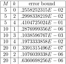
Now, we will try to check the “goodness” of the upper error bounds given in Corollary 4.2. For this purpose, we will take
(27) f(x) =f3(x) =
1
(cosx+M), |M|>1 in (10) and againp= 2. In this case one can write
f(x) = ˜f(eix) with f˜(z) = 2z
α k Interpolatory-type Szeg˝o DFT 1 0 .0003327230568994 .026901785277821 .501255163022280 1 3 .011034089407123 .366423427377691 .544879627889607 1 4 .04257230233186 .771276938936903 .605806335161480
.5 1 .002192800039399 .017545727235752 .571118102659482
.5 2 .009640505456589 .040265984545946 .593137505053635
.5 5 .185108978090672 .508365589525011 .881875249382593
.1 0 .000544431992941 .0001361725826865 .966599365120779
.1 3 .007729061901771 .002089448008441 .977513935435605
.1 4 .018247711351388 .004653758825189 .985752349128655 Table 3. A comparision of the relative errors in a 6-point Szeg˝o quadrature formula, a 11-point interpolatory-type rule with nodes the 11-th roots of 1 (both exact in Λ−5,5) and the discrete Fourier transform in the estimation ofG(wk) for
f1(x) given by (26).
α k Interpolatory-type Szeg˝o DFT
1 0 .000011127049588 .002531907754003 .511355152673849 1 1 .000006217099662 .014146717614614 .487521854761410 1 2 .000258217645989 .058756209807850 .518710579190526 1 3 .001107751936501 .252063738497163 .501965828743609
Table 4. A comparision of the relative errors in a 6-point Szeg˝o quadrature formula, a 11-point interpolatory-type rule with nodes the 11-th roots of unity (both exact in Λ−5,5) and the discrete Fourier transform in the estimation ofG(wk) for
f2(x) given by (26).
(observe that ˜f(z) = ˜f(1/z)) exhibiting two real poles given by y1 =
−M+√M2−1 andy
2=−M−
√
M2−1 =y−1
1 . Thus, in Corollary 4.2 one can take ̺1 < min{|y1|,|y1|−1} and ̺2 = ̺−11. Considering as above both Szeg˝o and interpolatory-type rules with the same domain of validity Λ−5,5, we observed numerically that the corresponding weights of the interpolatory-type quadrature formulas were positive and hence, the upper error bounds are equal for both procedures. The absolute errors of the numerical experi-ments implemented inMAPLEr 9.5 with 10 digits are displayed in Table 5. We can observe the “goodness” of these upper error bounds from the results presented in Table 5. Moreover, the more the modulus of the function
kf˜kΓ̺1∪̺2 in (24)–(25) increases, the greater the bounds are.
M k error bound 5 0 .2558252315E−02 5 2 .2998338219E−02 5 4 .4104725024E−01 10 1 .2876999356E−06 10 3 .1038596767E−03 10 4 .1973333858E−02 20 0 .3391315496E−07 20 2 .1076039338E−06 20 3 .6360698256E−06
Table 5. Upper error bounds in Corollary 4.2 for both Szeg˝o and interpolatory-type quadrature formulas with the same domain of validity Λ−5,5in the estimation of (10) withf(x) =
f3(x) given by (27) andp= 2.
we could also pass to the unit circle by using a Cayley transformation. For further details, see [3] where a more general set of orthogonal functions than polynomials, that is orthogonal rational functions, are studied and where such transformation allows one to recover properties for orthogonal rational functions from the real line to the unit circle, and vice versa. An analog of the method presented in this paper when the function f is not necessar-ily periodic and by passing from the whole real line to the unit circle by a Cayley transformation will be studied in a forthcoming paper.
References
[1] Handbook of mathematical functions with formulas, graphs, and mathematical tables. Edited by Milton Abramowitz and Irene A. Stegun. Reprint of the 1972 edition.Dover Publications, Inc., New York, 1992. xiv+1046 pp. ISBN: 0-486-61272-4. MR1225604 (94b:00012), Zbl 0643.33001.
[2] Bultheel, A.; Daruis, L.; Gonz´alez-Vera, P.Quadrature formulas on the unit circle with prescribed nodes and maximal domain of validity.J. Comp. Appl. Math.
231(2)(2009) 948–963. MR2549756 (2010i:65042), Zbl 1184.41015.
[3] Bultheel, A.; Gonz´alez-Vera, P.; Hendriksen, E.; Nj˚astad,O. Orthogonal rational functions. Cambridge Monographs on Applied and Computational Math-ematics, vol 5. Cambridge University Press, Cambridge, 1999. xiv+407 pp. ISBN: 0-521-65006-2. MR1676258 (2000c:33001), Zbl 0923.42017.
[4] Bultheel, A.; Gonz´alez-Vera,P.; Hendriksen, E.; Nj˚astad, O. Orthogonal rational functions and interpolatory product rules on the unit circle. II. Quadrature and convergence. Analysis, M¨unchen 18 (1998) 185–200. MR1625188 (99i:30054), Zbl 0929.30027.
[6] Bultheel, A.; Mart´ınez, H. Computation of the fractional Fourier trans-form. Appl. Comp. Harm. Anal.16(3) (2004) 182–202. MR2054278 (2005d:65250), Zbl 1049.65156.
[7] Cantero, M.J.; Cruz-Barroso. R; Gonz´alez-Vera, P. A matrix approach to the computation of quadrature formulas on the unit circle. Appl. Num. Math. 58
(2008) 296–318. MR2392689 (2009a:65052), Zbl 1139.65015.
[8] Cruz-Barroso, R.; Daruis, L.; Gonz´alez-Vera, P.;Nj˚astad, O. Sequences of orthogonal Laurent polynomials, bi-orthogonality and quadrature formulas on the unit circle. J. Comp. Appl. Math. 200 (2007) 424–440. MR2333724 (2008f:65042), Zbl 1136.42020.
[9] Cruz-Barroso, R.; Gonz´alez-Vera, P.; Perdomo-P´ıo, F. An application of Szeg¨o polynomials to the computation of certain weighted integrals on the real line. Numer. Algor.52(2009) 273–293. MR2563943 (2010j:65033), Zbl 1184.65031. [10] Cruz-Barroso, R.; Gonz´alez-Vera, P.; Perdomo-P´ıo, F. On the computation
of the coefficients in a Fourier series expansion.Innovation in Engineering Computa-tional Technology, 347–370.Saxe-Coburg Publ., Stirlingshire, Scotland,2006. [11] Cruz-Barroso, R.; Gonz´alez-Vera, P.; Perdomo-P´ıo, F. Orthogonality,
inter-polation and quadratures on the unit circle and the interval [−1,1].J. Comp. Appl. Math.235(2010) 966–981. Zbl pre05817748.
[12] Cruz-Barroso, R.; Gonz´alez-Vera, P.; Perdomo-P´ıo, F. Quadrature formulas associated with Rogers–Szeg˝o polynomials. Comp. Math. Appl.57 (2009) 308–323. MR2488385 (2009k:65040), Zbl 1165.65324.
[13] Cruz-Barroso, R.;Gonz´alez-Vera, P.; Nj˚astad, O. On bi-orthogonal systems of trigonometric functions and quadrature formulas for periodic integrands. Numer. Algor.44(2007) 309–333. MR2335805 (2008i:42003), Zbl 1129.65014.
[14] de la Calle Ysern, B.; Gonz´alez-Vera. P. Rational quadrature formulae on the unit circle with arbitrary poles. Numer. Math.107(2007) 559–587. MR2342643 (2008j:65028), Zbl 1136.65033.
[15] Gonz´alez-Vera, P.; Mart´ınez, H.; Trujillo, J. J. An application of Szeg¨o quadratures to the computation of the Fourier transform.Appl. Math. Comput.187
(2007) 183–194. MR2323568 (2008d:41024), Zbl 1121.65132.
[16] Gonz´alez-Vera, P.; Santos-Le´on, J. C.; Nj˚astad, O. Some results about numerical quadrature on the unit circle. Adv. Comp. Math. 5 (1996) 297–328. MR1414284 (98f:41028), Zbl 0856.41025.
[17] Gragg, W. B.Positive definite Toeplitz matrices, the Arnoldi process for isometric operators and Gaussian quadrature on the unit circle.Numer. Meth. Lin. Alg., 16–32. Moscow University Press, Moscow, 1982.
[18] Gragg, W. B. Positive definite Toeplitz matrices, the Arnoldi process for isometric operators and Gaussian quadrature on the unit circle. J. Comp. Appl. Math. 46
(1993) 183–198. This is a slightly revised version of [17]. MR1222480 (94e:65046), Zbl 0777.65013.
[19] Jones, W. B; Nj˚astad, O.; Thron, W. J. Moment theory, orthogonal polynomials, quadrature, and continued fractions associated with the unit circle. Bull. London Math. Soc.21(1989) 113–152. MR0976057 (90e:42027), Zbl 0637.30035.
[20] Jones, W. B.; Waadeland, H.Bounds for remainder terms in Szeg˝o quadrature on the unit circle.Approximation and computation(West Lafayette, IN, 1993), 325-342. Internat. Ser. Numer. Math., 119.Birkh¨auser Boston, Boston, MA, 1994. MR1333626 (96i:41029), Zbl 0818.41024.
[22] Levinson, N. The Wiener RMS (root mean square) error criterion in filter design and prediction.J. Math. Phys.25(1947) 261–278. MR0019257 (8,391e).
[23] Ozatkas, H. M.; Kutay, M. A.; Zalevsky, Z. The fractional Fourier transform. Wiley, Chichester, 2001.
[24] Simon, B. Orthogonal polynomials on the unit circle. Part 1. Classical theory. Amer-ican Mathematical Society Colloquium Publications, 54, Part 1.American Mathemat-ical Society, Providence, RI, 2005. xxvi+466 pp. ISBN: 0-8218-3446-0. MR2105088 (2006a:42002a), Zbl 1082.42020.
[25] Szeg˝o, G. On bi-orthogonal systems of trigonometric polynomials. Magyar Tud. Akad. Kutat´o Int. K¨ozl.8(1963) 255–273. MR0166541 (29 #3815).
[26] Szeg˝o, G.Orthogonal polynomials. Fourth edition. American Mathematical Society, Colloquium Publications, Vol. XXIII. American Mathematical Society, Providence, R.I., 1975. xiii+432 pp. MR0372517 (51 #8724).
Department of Mathematical Analysis, La Laguna University, 38271 La La-guna, Tenerife. Canary Islands. Spain.
Department of Mathematical Analysis, La Laguna University, 38271 La La-guna, Tenerife. Canary Islands. Spain.
Department of Mathematical Analysis, La Laguna University, 38271 La La-guna, Tenerife. Canary Islands. Spain.