T H E J O U R N A L O F H U M A N R E S O U R C E S • 45 • 4
Responsive to Distant Labor
Market Opportunities?
Abigail Wozniak
A B S T R A C T
Are highly educated workers better at locating in areas with high labor demand? To answer this question, I use three decades of U.S. Census data to estimate a McFadden-style model of residential location choice. I test for education differentials in the likelihood that young workers reside in states experiencing positive labor demand shocks at the time these workers entered the labor market. I find effects of changes in state labor demand on college graduate location choice that are several times greater than for high school graduates. Nevertheless, medium-run wage effects of entry la-bor market conditions for college graduates equal or exceed those of less-educated workers.
I. Introduction
College-educated workers in the United States are much more geo-graphically mobile than their less-educated peers when mobility is defined as making a long-distance move. For example, roughly 45 percent of college graduates reside out of their states of birth by age 30 as compared to only 27 percent of high school
1. For overviews of the literature on migration correlates, of which education is one, see Greenwood (1975) and Greenwood (1997).
Abigail Wozniak is a professor of economics at the University of Notre Dame and is affiliated with NBER and IZA. She thanks the Social Sciences Research Council, the Thomas Cochran Dissertation Fellowship in Economic and Business History, and Harvard University for support during the course of this research. The author has benefited from numerous helpful conversations with Lawrence Katz, Clau-dia Goldin, David Cutler, Caroline Hoxby, Adriana Lleras-Muney, Ofer Malamud, Raven Saks, Lucie Schmidt, James Sullivan, Tara Watson, Neal Wozniak. and seminar participants at the Harvard Eco-nomics Department Labor and Public EcoEco-nomics Lunch, the University of Notre Dame, Williams Col-lege, the Federal Reserve Bank of Philadelphia, and IZA. The author takes responsibility for all errors, omissions, and oversights. The data used in this article can be obtained beginning June 2011 through May 2014 from Abigail Wozniak, Department of Economics, University of Notre Dame,
a_wozniak@nd.edu.
[Submitted May 2008; accepted May 2009]
graduates.1 Given these large differences in migration levels, it is reasonable to wonder whether college graduates are also relatively better at moving to take ad-vantage of variation in local labor market conditions.
I address this question and two others in this paper. First, I ask whether the location choices of college graduates are more sensitive to local labor market con-ditions than those of their less-educated peers. If so, does their choice of local market have any lasting effects on their wages? And finally, is the location response to local conditions driven by an individual’s current market conditions or do other markets exert similar push/pull effects? Taken together, this analysis provides insight into how location choice in response to labor market arbitrage opportunities contributes to educational differences in outcomes.
The empirical analysis focuses on recent labor force entrants. Using microdata from the 1980, 1990, and 2000 U.S. Censuses, I match workers observed in their late twenties to the set of state conditions they faced when entering the labor market. I construct two sets of measures of state labor market conditions, which include measures for both short- and medium-run changes in conditions. The first is based on a measure of state labor demand changes developed by Bartik (1991). These measures are purged of state employment changes resulting from labor supply shifts, an important consideration in this context. The second set of measures uses state unemployment rates as indicators of entry labor market conditions. The unemploy-ment rate measures are not purely exogenous to migration decisions, but they retain some of the demand variation that is removed from the Bartik measures. I also construct education group specific versions of all measures to account for variation in labor market opportunities across groups but within states.
I find that better entry labor market conditions in a state disproportionately attract college-educated workers, particularly college graduates. In my preferred specifica-tions of the conditional logit model, a standard deviation improvement in state entry labor market conditions increases the probability that a college graduate chooses a state by roughly 5–15 percent. The second part of the paper uses wage equations to test for lasting impacts of the entry labor market conditions that individuals expe-rienced. The results here are somewhat surprising. Despite their greater propensity to undertake arbitrage migration, I find only modest evidence of any arbitraging impacts on the wages of college graduates. In fact, when entry labor market con-ditions are measured in an education-specific manner, college graduates experience average wage impacts of these conditions that are as large or larger than those for high school graduates. Finally, I find evidence that individual location choices re-spond more or less equally to conditions in all states. This is true regardless of educational attainment. The effects of local labor market conditions on location choice do not appear to be driven solely by responses to conditions in an individual’s state of residence at the time of the labor market shocks.
These results have implications for several literatures. The first examines the im-pact of shocks to local economic conditions on relative outcomes. A number of studies in this literature find that less-skilled workers suffer more severe and longer-lasting effects of poor local economic conditions (Topel 1986; Topel 1994; Bound and Holzer 2000; Black, McKinnish, and Sanders 2005).2Adjustment of the local
labor supply through migration is thought to be an important channel through which relative outcomes are affected by local shocks (Blanchard and Katz 1992).3If more-educated workers migrate to areas with greater labor market opportunity, migration will reduce the impact of poor local conditions on their outcomes. Bound and Holzer (2000) provide strong evidence of this pattern in the 1980s. My work shows that the greater responsiveness of more-educated workers is a more general phenomenon, observed here over 30 birth year cohorts in a model of individual location choice. I also show that all workers experience significant lasting wage impacts of conditions in the market they choose to enter and that workers respond to conditions in all possible choice states, not just their current market. This suggests that the finding of migration-induced wage arbitrage in Bound and Holzer (2000) and others may be sensitive to the particular measures of local conditions they use.
My work also has implications for the “scarring effects” literature—papers that find medium- to long-run effects of prior labor market conditions on wages (Ellwood 1982; Gardecki and Neumark 1998; Kletzer and Fairlie 2003; Kahn 2008; Ore-opoulos, von Wachter, and Heisz 2006).4Most of these studies find significant wage impacts of early conditions that last 5–10 years into a worker’s career. I find that scarring effects are still present even when workers are better at undertaking arbi-trage migration. Workers simply experience “scarring” consistent with the market they choose to enter. Moreover, using measures of entry labor market conditions targeted to particular education groups is key to this finding.5This has implications for theories of scarring effects (Harris and Holmstrom 1982; Beaudry and DiNardo 1991). In particular, it suggests that the usual process of job transitions may be more important than migration for eroding the wage effects of initial conditions.6
Finally, this paper also adds to our knowledge about educational differences in migration rates. The fact that higher education is a strong correlate with migration within the United States has long been established. Greenwood (1975) and Green-wood (1997) are just two examples. Malamud and Wozniak (2008) argue that there is a causal relationship behind this correlation. Little else is known about the origins of this differential.
II. The Young Worker’s Migration Decision
To understand how an individual chooses a local labor market, con-sider how she balances the costs and benefits to moving between markets. For a worker residing in states*, the choice problem is the following:
3. A literature that is similar in spirit examines the migration responses of the poor to state variation in benefits (Meyer 2000; Gelbach 2004). In general the magnitude of these responses is fairly modest. See Kennan and Walker (2008) for a structural model of how expected future wages affect migration. 4. Oyer (2006) and Bender and von Wachter (2006) find scarring effects in more specialized labor markets. 5. This is likely the reason for the difference between my findings on this point and those in Genda, Kondo, and Ohta (2010).
E(w(e) )st t
arg maxU()⳱arg max ␦(e) ⳮc(e) (1s⬆s*) ⳮ␣(e) (1s⬆s*)
(1) s
冦
兺
冤
(s,s*)t冥冧
(s,s*)p
s僆S s僆S t st
whereindicates consumption; (s,s*) forms a destination and origination state pair; sindexes the other 50 states;tindexes time periods;eindexes education groups;w is the nominal wage in states,pis the price level ins; and␦is a discount rate that may depend on education.c and␣are recurring and one-time costs (respectively) that a worker must incur if he chooses to supply labor in a state other than his current states*. In theory these also may depend on education. The origins of fixed moving costs are fairly obvious—truck rentals, etc. Recurring costs include things like the psychic costs of being away from old friends and family or in an environ-ment where one does not feel like a “native” as well as the monetary costs of return visit travel or of maintaining a home with guest accommodations.
If expected benefits from residing in some s exceed costs to moving from s*to s, the worker moves across local markets. The probability that a worker makes such a move is increasing in the expected wages available in statess ⬆ s*. To see this,
simplify Equation 1 by assuming that the cost cis the same in every period and is independent of the destination and origin state pair (s,s*) and of education.Assume that␣is similarly independent of the migration route and education and that prices do not differ across states. Then the probability that a worker chooses to supply labor in state s⬆s*depends on conditions in s as well as conditions in all other
states –sin the following way:
Pr (choose s⬆s*)⳱ (2)
Pr
冤
兺
(E(w(e) )stⳮc)ⳮ␣兺
E(w(e) )s*t and兺
E(w(e) )st兺
E(w(e)ⳮst)冥
∀s,ⳮs⬆s*t t t t
This is now a standard choice problem, like those considered by McFadden (1974).7The McFadden choice framework offers a clear prediction about how in-creases in E(w(e)st) should affect migration choices of utility maximizing agents—
increasesE(w(e)st) in should increase the probability that statesis chosen by
mem-bers of group e at time t, all else equal. The conditional logit model developed alongside this choice framework offers an empirical setting in which to test this prediction.
III. Data Series and Empirical Methodology
I focus on the location choices of young workers because they form the most geographically mobile segment of the labor force. A focus on young work-ers also minimizes the complicated family and lifecycle considerations that might affect the migration choices of older workers. I match young workers to proxies for changes in expected wages that occurred as they were entering the labor market for
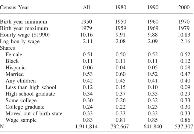
Table 1
Descriptive Statistics
Census Year All 1980 1990 2000
Birth year minimum 1950 1950 1960 1970
Birth year maximum 1979 1959 1969 1979
Hourly wage ($1990) 10.16 9.91 9.88 10.83
Log hourly wage 2.11 2.08 2.09 2.16
Shares
Female 0.51 0.50 0.52 0.52
Black 0.11 0.11 0.11 0.12
Hispanic 0.06 0.04 0.05 0.08
Married 0.53 0.60 0.52 0.47
Any children 0.42 0.45 0.41 0.40
Less than high school 0.12 0.15 0.10 0.09
High school graduate 0.34 0.37 0.35 0.29
Some college 0.30 0.26 0.32 0.33
College graduate 0.24 0.22 0.23 0.30
Moved out of birth state 0.33 0.33 0.33 0.33
Wage sample 0.83 0.81 0.85 0.86
N 1,911,814 732,667 641,840 537,307
Notes: Data are taken from IPUMS versions of U.S. Census 5 percent samples for 1980, 1990, and 2000. Sample is noninstitutionalized U.S. natives with 5–8 years of potential labor market experience as defined in text.
the first time. Thus, the proxies represent changes in expected wages on an individ-ual’s first job after completing her schooling.
A. The U.S. Census Microdata Sample
My data come from the 5 percent Integrated Public Use Micro Sample of the U.S. Census (hereafter IPUMS; Ruggles and Sobek 2003) for the Census years 1980, 1990, and 2000. I define young workers as those who have 5–8 years of potential labor market experience at the time of the Census. I divide individuals into four education groups: dropouts who have not completed a high school degree or GED; high school graduates and GEDs; some college, which consists of those with one to three years of some kind of post-secondary education; and college graduates, who have a bachelor’s degree or higher. I calculate potential labor market experience using the Mincer formula: age minus years of schooling minus six.8Limiting the sample to workers with 5–8 years of experience means that a given birthyear cohort appears only once in my sample, as shown in the birth year statistics in Table 1.
The sample is further restricted to noninstitutionalized U.S. natives with nonimputed states of birth and hourly wages of more than one dollar and less than $100 in constant 1990 dollars.9
Limitations of the Census data require me to focus on a worker’s choice of local labor market at the state level. The IPUMS Census extracts are large, representative samples of the U.S. population that offer snapshots of young workers over several decades, but the geographic mobility information on respondents is limited. The Census records state of birth and state of residence at the time of the Census, so one can observe both choice of state of residence and migration out of the birth state. In specifications where I examine a migration probability, rather than a location choice, I use out of birth state residence as my migration measure.10
One concern with the use of cross-sectional data is that some individuals will have moved out of their birth states as children. If the probability of childhood migration is similar across education groups, this measurement error will only at-tenuate estimates of the effect of state conditions. A bigger concern is that more and less-educated individuals may be differentially likely to reside outside their state of birth prior to age 18. More-educated individuals tend to have more-educated parents, who in turn may have moved their children out of their birth states. Using data from the geocoded NLSY 1979, which contains longitudinal information on state of res-idence, I have found that this concern is not supported by the data. College graduates are somewhat more likely than high school graduates to reside outside their states of birth in their late teens, but the difference is small compared to the level of out of birth state residence among teenagers overall. The educational gap in out of birth state migration really opens up in adulthood. A related concern is that more-educated parents may move their children to states that will be better performing when the children enter the labor market. In this case, parental choices would make it appear that their more-educated offspring are more responsive to state conditions than other early career workers. However, I find that as teenagers, college graduates in the NLSY79 are no more likely than high school graduates to reside in a state that will have better labor market conditions at the time they enter the labor force.11
Table 1 presents summary statistics for relevant variables from the IPUMS sample by Census year. The share of blacks and women is highly stable across cohorts and years in my sample. Consistent with well-known trends, the fraction Hispanic in-creases and the fractions currently married or with children present in the household decrease in more recent cohorts.12The average tendency to reside outside one’s birth
9. According to IPUMS staff, observations requiring imputation of birth states were most likely a random subset.
10. The Census also records location of residence five years ago. I prefer the migration measure based on out of birth state migration because an individual’s birth state is exogenous to expected entry labor market conditions.
11. Results in this paragraph available upon request.
state is stable across cohorts. Real wages are stable throughout my sample, but the share of individuals meeting the wage restrictions increases from 81 percent in the 1980 cohorts to about 85 percent in 1990, and 2000. This is likely due to a higher share of individuals with zero earnings during the poor labor market of the late 1970s and early 1980s. All migration results are robust to including individuals who do not meet the wage sample restrictions in the estimations.
B. Measuring Entry Labor Market Conditions
To test for differences in migration responses to early career local labor market conditions, I require a set of changes in these conditions that do not affect education choices. These changes also should be driven by increases in labor demand, so as to avoid the confounding effects of changes in local labor supply in explaining location choices.
A method of isolating local labor demand changes was developed in Bartik (1991) and is sometimes called the Bartik instrument. This approach has since been em-ployed by Blanchard and Katz (1992), Bound and Holzer (2000), and Saks (2008). The Bartik measure averages national employment growth across industries using local industry employment shares as weights to produce a measure of local labor demand that is unrelated to changes in local labor supply.
Drawing on Bartik’s measure, I create the following measure of annual state labor market conditions:
J
˜ ˜
Bartik e
(
lnE ⳮlnE)
(3) st兺
sjtⳮ1 jt jtⳮ1j⳱1
wherejindexes industry,sstate, and tyear. The term in parentheses is a measure of industry j employment growth nationally. Specifically, it is the log of national employment injexcluding statesemployment in that industry (E˜jt), divided by the same quantity in the previous year (E˜jtⳮ1). esjt-1is the share of statesemployment
in industry jin year t-1. It is applied as a weight to the log national employment growth term. The sum of these industry-level products proxies for changes in state level employment driven by industry growth outside the state. I constructed the series using data on state industry employment from the Bureau of Economic Analysis (BEA). The BEA data span 1969 to 2000 and maintain a consistent set of industry codes throughout. The industry detail in the BEA series is a hybrid of two- and three-digit SIC levels.
One concern with the measure in Equation 3 is that a given shock may not reflect the same change in conditions for workers of all education levels. For example, Bound and Holzer (2000) note that variation in their versions of the Bartik measures is driven largely by fluctuations in manufacturing employment. To better approxi-mate changes in labor market conditions affecting specific education groups, I con-struct an alternate version of the measure in Equation 3. This takes the following form:
J
˜ ˜
Ed_Bartik w e
(
lnE ⳮlnE)
(4) kst兺
ksjd t( ) sjtⳮ1 jt jtⳮ1Herekindexes the four education groups.wksjd(t)are weights constructed from older cohorts (workers ages 36–55) from the same IPUMS 5 percent samples of the 1980, 1990, and 2000 Censuses. The weights are equal to the share of education group k’s statesemployment that is in industryjin a particular decaded(t). The shares are computed using the older sample of workers to avoid the confounding effect of supply shifts of young migrants. d(t) assigns the weights computed from the three Census years to the annual BEA series of industry weights and log employment changes on a decadal basis.
I match individuals in the Census microdata to theBartikandEd_Bartikmeasures for the year they likely entered the labor market, where labor market entry year is based on reported education.13I also create five-year moving averages ofBartikand Ed_Bartik and match those to individuals whose assigned labor market entry year is the center of the moving average. The Ed_Bartik measures are of course also matched on education. The 5-year averages provide a somewhat different picture of early labor market conditions than the single year measures. The Bartik measures capture medium-run changes in state labor market conditions, while the single year measures reflect more immediate, short run changes. Workers may respond more strongly to one or the other in making their location decisions. The 5-year measures also may do a better job of capturing relevant conditions if workers have some flexibility in choosing when to enter the labor market.
A concern with the Bartik measures is that they may only reflect part of the changes to state labor market conditions at any given time. For this reason I also present results using state unemployment rates to measure early labor market con-ditions. As before, I use both the labor market entry year unemployment rate and the 5-year moving average around that year. I also construct an education-specific state unemployment rate using CPS MORG data for the period 1979–2000.14 In using unemployment rates, I trade off an unconfounded measure of state labor mar-ket conditions for one that potentially captures a broader set of economic conditions and of which workers may be more aware. Note that the supply response to low unemployment rates will tend to attenuate any wage impacts of these conditions since workers who move into low unemployment areas with high wages raise the local unemployment rate and confound the relationship between local unemployment conditions and wages. The same attenuating effect works in the opposite direction as workers move away from high unemployment rate, low wage areas.
Finally, one might worry that choices about completed education are affected by early career labor market conditions. Workers who face a bad labor market may choose to stay in school longer, hoping that conditions will improve. The compo-sition of education groups will then vary depending on a cohort’s assigned labor market entry year. As a result, responses of an education group at one point in time would not be directly comparable to behavior of the same group at another time.
13. I assign everyone a labor market entry year equal to their birth year plus 6 plus assumed years of schooling.
To examine this possibility, I regressed the sample shares in four educational at-tainment categories computed by birth state and birth year on cell average labor market conditions and cell percents black, Hispanic, female, married, and children present, plus a complete set of birth state and birth year dummies. I find no evidence that changes in educational attainment in response to labor market conditions are a concern in this context.
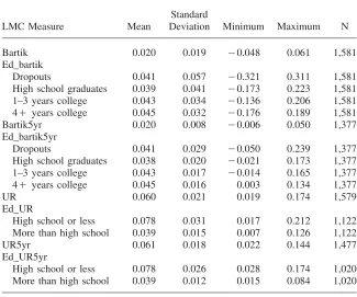
Table 2 presents descriptive statistics on the measures used to assess early labor market conditions. In the analysis, the education-specific measures are matched to individuals depending on their education level, but these measures are summarized separately here. (Ed_Bartik appears as a single measure in regressions.) Panel A shows that, as expected, the five-year moving averages have less variance than their underlying annual measures. Recall that as shown in Equation 4, the education-specific Bartik measures are constructed by premultiplying the elements of the Bartik measure by quantities that are all less than one but that sum to one within a state, education group, and year cell. This has two consequences for comparing the edu-cation-specific measures withBartik.First, the scale is no longer comparable, since the premultiplying “shrinks” the Bartik components. The education-specific mea-sures in Table 2 have been rescaled (multiplied by 100) to make their means com-parable in scale to those ofBartik andBartik5yr. Second, since the weights apply withineducation groups instead of across them, the Bartik measures are not averages of the education-specific measures.15 One should consider the education-specific measures to be an alternative index of conditions designed to apply to particular education groups rather than a subset of the conditions averaged into the Bartik measures. The education-specific measures are, however, comparable with one an-other. Panel A also shows higher levels of unemployment and higher variance in the education-specific Bartik and unemployment measures for less-educated workers. Because of these issues, the measures of entry labor market conditions fall into three distinct categories: Bartik measures, education-specific Bartik measures, and unemployment rate measures (both overall and within education groups). Panel B shows correlations across selected measures. The modest levels of correlation (with the exception of the UR and UR_5yr correlation) suggest that the measures reflect related but not identical conditions in state labor markets. The distinct nature of the measures also makes direct comparison of results across measures problematic. In the analysis, these measures will all be standardized to have mean zero and standard deviation of one. This way it will be easy to see whether a one standard deviation in conditions measured byXhas a different impact than a standard deviation change in conditions measured byY. WhetherXandYrepresent the same conditions or the same change in conditions in a deeper sense is beyond the scope of this paper.
C. Analyzing Choice of Residence State Using the Conditional Logit Model
To examine the responsiveness of education groups to state labor market conditions, I estimate a model of the individual choice problem in Equation 2 using McFadden’s
Table 2
Measures of State Labor Market Conditions
Panel A
Descriptive Statistics (Unweighted)
LMC Measure Mean
Standard
Deviation Minimum Maximum N
Bartik 0.020 0.019 ⳮ0.048 0.061 1,581
Ed_bartik
Dropouts 0.041 0.057 ⳮ0.321 0.311 1,581
High school graduates 0.039 0.041 ⳮ0.173 0.223 1,581 1–3 years college 0.043 0.034 ⳮ0.136 0.206 1,581 4Ⳮyears college 0.045 0.032 ⳮ0.176 0.189 1,581
Bartik5yr 0.020 0.008 ⳮ0.006 0.050 1,377
Ed_bartik5yr
Dropouts 0.041 0.029 ⳮ0.050 0.239 1,377
High school graduates 0.038 0.020 ⳮ0.021 0.173 1,377 1–3 years college 0.043 0.017 ⳮ0.014 0.165 1,377
4Ⳮyears college 0.045 0.016 0.003 0.134 1,377
UR 0.060 0.021 0.019 0.174 1,579
Ed_UR
High school or less 0.078 0.031 0.017 0.212 1,122 More than high school 0.039 0.015 0.007 0.126 1,122
UR5yr 0.061 0.018 0.022 0.144 1,477
Ed_UR5yr
High school or less 0.078 0.026 0.028 0.174 1,020 More than high school 0.039 0.012 0.015 0.084 1,020
Panel B
Correlations across Measures (Unweighted)
Bartik Bartik5yr UR UR5yr
Bartik 1.00
Bartik_5yr 0.50 1.00
UR ⳮ0.29 ⳮ0.16 1.00
UR_5yr ⳮ0.11 ⳮ0.16 0.93 1.00
conditional logit representation (McFadden 1974).16McFadden’s model allows each individual to choose from among J unordered choices 1, 2, . . . , J. In the case of choosing a state of residence,J⳱50 and individuals are restricted to choosing only one. Therefore if yij is an indicator representing an individual’s decision regarding
state j, then yij⳱1 ifjis the chosen state, 0 otherwise, andjyij⳱1 for every i.
Let yi ⳱ (yi1,yi2, . . .yi50) describe i’s decisions on all his possible choice options. Then the conditional probability of observingyiis the following:
50 exp
冢
兺
y xij ij冣
50
j⳱1 Pr y y⳱1 ⳱
(5)
冢
i兺
ij冣
50j⳱1
exp d x
兺
di僆Si冢
兺
ij ij冣
j⳱1Under the assumptions explained in McFadden (1974), this expression equals the probability that a chosen statejprovides greater utility toithan all other nonchosen statesj⬘. The exponent terms and their arguments come from the familiar parame-terization of the logistic regression model for binary outcomes. Siis the set of all
possibleyioutcomes, which are denoteddi. xijis a vector of characteristics of choice
j, which also may depend on individuali’s characteristics. Note that characteristics xithat do not vary with choicejin thexijvector would simply drop out of the right
hand side expression in Equation 4. For this reason, only characteristics that vary across choices are included in the conditional logit estimations.17
The coefficient vector is estimated by maximizing the conditional probability of observing yiusing the following log-likelihood function:
N 50 50
lnL⳱ y xⳮln exp d x (6)
兺 兺
冦
ij ij冢
兺
冢
兺
ij ij冣冣冧
n⳱1 j⳱1 di僆Si j⳱1
where the data contain observations on the choices of N individuals.18
The conditional logit specification includes the following controls: a measure of state labor market conditions (LMC), which is one of the measures defined in the previous subsection; interactions of LMC with education, gender, race and ethnicity; distance from birth state; an indicator for birth region; long-term average income in the state for the individual’s education group; lagged education-specific migration flows from the birth state; dummy variables for each potential choice state; and choice state region times birth year fixed effects.
The LMC measure and its interactions with education are the main covariates of interest. Specifically, the interactions areLMC gwhereiindexes individuals,
•educ
jb i
j indexes potential choice state, and b indexes year of birth. Educi
g are dummy
16. Other examples of the implementation of this model in migration settings include Davies et al. (2001); Knapp et al. (2001); and O’Keefe (2004).
17. In this sense, estimates ofobtained from McFadden’s conditional logit are robust to the inclusion of fixed individual characteristics. See McFadden (1974) for a discussion of this.
variables that indicate whether i is a member of each of four education groups indexed byg.
Distance from birth state, the dummy for division of birth, and long run migration flows capture stable migration relationships between an individual’s birth state and the potential choice states. Distance between the choice state and birth state is mea-sured as hundreds of miles between the two state capitals. The indicator for whether a potential choice state is in an individual’s division of birth accounts for the pull of nearby states and varies across birth state-destination state pairs. The lagged flows account for the pull forces generated by previous migration patterns. These include long-term trends such as migration to the South and to the coasts as well as numerous other important but less obvious state-to-state migration trends.19Importantly, these flows also capture “spurious” movements between states that result from metropol-itan areas that span more than one state. The flow measure between birth statea and residence state bequals the share of 31–35 year old natives ofaresiding inb at the time of the Census, conditional on educational attainment. If b⳱a this is simply the share of natives continuing to reside in their birth state.
Finally, fixed effects for potential choice states capture stable differences across states in terms of their attractiveness for migrants. These state fixed effects also account for states that have relatively diversified economies that contain more than one distinct labor market. State-wide conditions may be relatively poor measures of the relevant local labor market conditions in these states. Choice state region times birth year fixed effects account for aggregate conditions common to all cohorts.20
IV. The Effects of Labor Market Conditions on State
of Residence Choices
Before going into estimates of the conditional logit model, I estimate a linear probability model of a binary location decision: the zero-one choice of whether to reside outside one’s state of birth. The model is the following:
g g
move ⳱ⳭLMC Ⳮeduc Ⳮeduc *LMC
(7) isb 0 1 sb i i sb
g s g b
ⳭXⳭeduc *␦Ⳮeduc *␦ Ⳮε
i i i i i isb
The dependent variable is a dummy equal to 1 if individual iborn in state sin year bresides outside her state of birth when I observe her in the Census. LMC is one of the measures of birth state labor market conditions at individual i’s time of labor market entry. As in the conditional logit model, educgi represents a set of
dummies for four education groups. The main effect is included, as are interactions of the education group dummies with a full set of state of birth and year of birth fixed effects,␦i
sand␦ i
b, respectively. The vector of personal characteristicsX
iincludes
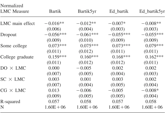
Table 3
Estimates of the Linear Probability Migration Model
Panel A
Bartik Measures of Birth State Labor Market Conditions (LMC)
Normalized
LMC Measure Bartik Bartik5yr Ed_bartik Ed_bartik5yr
LMC main effect ⳮ0.016** (0.006)
R-squared 0.057 0.058 0.057 0.058
N 1.60EⳭ06 1.60EⳭ06 1.60EⳭ06 1.60EⳭ06
(continued)
controls for race, Hispanic ethnicity, sex, marital status, and presence ofi’s children in the household.
Despite its limitations on the choice variable, this model has features that com-plement the subsequent analysis. First, the estimating equation is the same as the estimated wage equation, except of course for the dependent variable. This makes comparisons between wage and migration effects more transparent. Second, this model allows direct inclusion of cohort fixed effects, which are precluded by the form of the conditional logit since they do not vary across choice states.
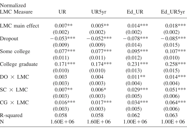
Table 3(continued)
Panel B
Unemployment Rate Measures of Birth State Labor Market Conditions (LMC)
Normalized
LMC Measure UR UR5yr Ed_UR Ed_UR5yr
LMC main effect 0.007**
R-squared 0.058 0.058 0.062 0.063
N 1.60EⳭ06 1.60EⳭ06 1.00EⳭ06 1.00EⳭ06
Notes: Data are taken from IPUMS versions of U.S. Census 5 percent samples for 1980, 1990, and 2000. Sample is noninstitutionalized U.S. natives with 5–8 years of potential labor market experience and positive wages in the previous year. All specifications include dummy variables for sex, race (Black/White), His-panic ethnicity, marital status (married or not), and children (present or not). Education group specific birth state and birth year fixed effects are also included.
graduate’s probability of residing in her birth state by about 1.6 percentage points, but the effect for other workers is only half this, about 0.75 percentage points. These results are somewhat surprising in that they imply that less-educated workers are more responsive to conditions that reflect average labor market changes than to those that reflect changes in their specific labor market opportunities. I return to this puzzle in the next section.
of staying by 38 percent more for college graduates than high school graduates. Results in which the probability changes significantly more than the average for college graduates will magnify this difference dramatically.
Panel B of Table 3 uses the unemployment rate measures to estimate Equation 7. Consistent with Panel A, the coefficients on the main effect show that workers who faced worse entry labor market conditions are more likely to leave their birth states across the four unemployment rate measures. (Note that the expected signs are re-versed across the Bartik and UR measures.) The impact of a standard deviation increase in entry unemployment rates is to raise the probability of leaving by 0.5 to 1.8 percentage points. There are also significant differences in the response to these conditions across education groups. College graduates and those with some college are significantly more likely to leave in all specifications, with larger effects on college graduates. A standard deviation increase in UR and UR5yr increases the probability that an individual with some college leaves his birth state by a little more than 1 percentage point, and that a college graduate leaves by more than 2 percentage points as compared to 0.5 percentage points for high school graduates.
Responses of those with some college or a college degree to conditions as mea-sured by education-specific unemployment rates are even larger. A standard devia-tion increase in these measures increases the probability that a skilled individual leaves his birth state by roughly 4.4 to 7.3 percentage points in total.21To convert these into changes in the probability of staying in one’s birth state, consider the Ed_UR5yrspecification. A standard deviation increase in this measure decreases the probability that a high school graduate stays from 0.75 to 0.732, a decrease of 2.4 percent. The same shock decreases a college graduate’s probability of staying from 0.55 to 0.486, a change of about 12 percent, or six times the change for a high school graduate.
Results from the linear probability model show that entry labor market conditions in the birth state affect the location choices of young workers. College graduates also appear to be more sensitive to these conditions than other education groups. But do entry labor market conditions in other states have a similar impact on an individual’s location choice? Or are individuals uniquely attuned to conditions in their birth states?
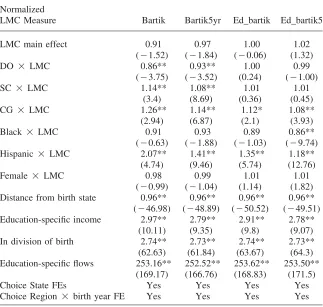
The conditional logit specification allows me to answer these questions. Results from its estimation are presented in Tables 4a and 4b. The top numbers in each cell are odds ratios implied by the estimated coefficients (unreported).22Z-statistics based on standard errors clustered on labor market entry year are in parentheses.23Due to the significant computational requirements of estimating the conditional logit, I use
21. The significant interaction of dropout and LMC in the education-specific unemployment rate specifi-cations is not robust. It reverses sign in the conditional logit specification.
22. Note that an odds ratio equal to one indicates that the dependent variable has no effect on an indi-vidual’s odds of choosing a state.
Table 4a
Estimates from the McFadden Conditional Logit State Choice Model
Normalized
LMC Measure Bartik Bartik5yr Ed_bartik Ed_bartik5
LMC main effect 0.91 Distance from birth state 0.96**
(ⳮ46.98) In division of birth 2.74**
(62.63)
Choice State FEs Yes Yes Yes Yes
Choice Region⳯birth year FE Yes Yes Yes Yes
Notes: Top number in cell is implied odds ratio. Z-statistics computed using clustered standard errors on labor market entry year are in parentheses. * indicates significance at the 5 percent level, ** at the 1 percent level. Data are taken from IPUMS versions of U.S. Census 5 percent samples for 1980, 1990, and 2000. Sample is noninstitutionalized U.S. natives with 5–8 years of potential labor market experience and positive wages in the previous year. Observations used in estimation were a random 50 percent sample of the sample used in Table 3.
a 50 percent random sub-sample of the Table 3 sample to estimate the equations in 4a and 4b.
Odds ratios in the top row of Table 4a show that the Bartik measures have no detectable effects on the likelihood that a high school graduate chooses to reside in any given state.24 College-educated individuals, however, show significant,
signed responses to state conditions. The odds ratios on the interactions of LMCs with dummies for some college and college graduate are greater than one in both the Bartik and Bartik5yr specifications. Since odds ratios are multiplicative rather than additive, these results show that individuals with some college education are more sensitive to entry labor market conditions in a state than are high school graduates. For an individual with some college, a standard deviation increase in these measures boosts the odds implied by the main effect by 8–14 percent. For college graduates, the boost is 14–26 percent. In total, a standard deviation increase in Bartik-measured LMCs leads to an 11–14 percent increase in the odds of a college graduate choosing a state, as compared with no effect for high school graduates. Using the education-specific Bartik measures, the only significant education group interaction is with college graduate. The total effects here are similar to those in the Bartik specifications, with a standard deviation increase in LMCs leading to about a 12 percent increase in the overall odds that a college graduate chooses a state.
Coefficients on other included controls largely have the expected signs. Distance from birth state decreases the odds that an individual chooses a particular state, while education group long term income, location within one’s division of birth, and the historical migration flow of one’s education group to a state all increase the odds of choosing it. The gender difference in response to these conditions is insignificant in all specifications. Blacks have a weakly wrong-signed response to Bartik-mea-sured LMCs while Hispanics are more responsive, roughly on the same order of magnitude as college graduates, although some of these race/ethnicity interactions change signs and significance in the unemployment rate specifications.
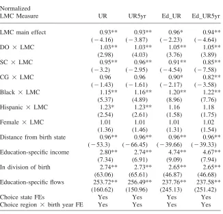
Table 4b presents estimates of the conditional logit model using the unemploy-ment rate measures of entry labor market conditions. Since increases in a state’s unemployment rate should make it less attractive, we expect odds ratios of less than one on the main effect. This is what I find in the first row of Table 4b. A standard deviation increase in the unemployment rate lowers the odds of an individual choos-ing a state by about 6 percent. Dropouts are less responsive than this, while college-educated individuals are more responsive (although the college graduate interaction with LMC is only significant using the education-specific unemployment rates). A standard deviation increase in unemployment conditions reduces the odds of a col-lege-educated individual choosing a state by about 10–20 percent overall.
To test whether the results in Tables 4a and 4b are driven by birth state conditions alone, I reestimated the specifications in 4a and 4b adding interactions of the LMC main effect and its education interactions with an indicator for whether the choice state was an individual’s birth state. (I also included the main effect of birth state.) Coefficient estimates and significance patterns on the LMC main effect and educa-tion group interaceduca-tions were essentially unchanged in this exercise. In fact, the wrong signed coefficients on the main effect in theBartikandBartik5yrspecifications are driven by wrong signed responses to birth state conditions in these models. If the response to birth state conditions alone were driving the estimates in the first four
theirproduct, so the total effect of LMCs on college graduates in theBartikspecification is 0.93⳯1.338 ⳱1.24. In other words, a 34 percent increase over the main effect odds means that a one unit change in
Table 4b
Estimates from the McFadden Conditional Logit State Choice Model
Normalized
LMC Measure UR UR5yr Ed_UR Ed_UR5yr
LMC main effect 0.93** Distance from birth state 0.96**
(ⳮ53.3) In division of birth 2.74**
(63.06)
Choice state FEs Yes Yes Yes Yes
Choice region⳯birth year FE Yes Yes Yes Yes
Notes: Top number in cell is implied odds ratio.Z-statistics computed using clustered standard errors on labor market entry year are in parentheses. * indicates significance at the 5 percent level, ** at the 1 percent level. Data are taken from IPUMS versions of U.S. Census 5 percent samples for 1980, 1990, and 2000. Sample is noninstitutionalized U.S. natives with 5–8 years of potential labor market experience and positive wages in the previous year. Observations used in estimation were a random 50 percent sample of the sample used in Table 3.
rows of 4a and 4b, then interactions of these covariates with birth state would be of similar magnitude and significance as the reported estimates. Instead, the interactions with birth state are rarely significant, although birth state itself is.25These results imply that individuals give equal weight to states’ entry labor market conditions in choosing their residence state.
Are the responses estimated in Tables 4a and 4b large or small? On the face of it, a roughly 15 percent change in the odds (as implied by both the education-specific Bartik and UR measures) that a college graduate chooses a state seems large, but assessing the magnitude of these estimates requires that odds ratios be converted into probabilities. If a state initially has a 0.55 probability of retaining a college graduate (which is what the sample means suggest), then that probability improves to 0.58 following an improvement in entry labor market conditions that improves relative odds by 15 percent.26This represents a 5.4 percent increase in the probability of retaining a college graduate. On the other hand, if a state has a 2 percent chance of attracting a random college graduate, say from another state, then the same change increases this probability to 0.023, an increase of about 15 percent.27
V. Does the Response to Local Conditions Affect
Labor Market Outcomes?
In Table 5, I test whether conditions in a worker’s birth state at the time he entered the labor market are a significant determinant of his wages 5–8 years later, when I observe him in the Census data. There are reasons to expect no lasting wage effects. If the migration flows in Tables 3, 4a, and 4b are large enough, wage effects of labor market entry conditions will be arbitraged away early in a worker’s career. Alternatively, wages may adjust as labor market conditions change over a worker’s career. In this case, wage effects of conditions at a point in time may not be fully arbitraged by migration, but subsequent conditions may supersede the effects of early conditions. On the other hand, lasting wage effects imply that neither of these forces is sufficient to eliminate the medium-run effects of entry labor market conditions.
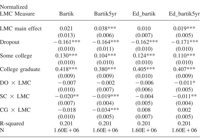
Table 5 estimates the wage equation obtained by substituting log real hourly wages for the migration dummy in the left hand side of Equation 7. Panel A, which uses the Bartik measures, shows that it is mainly the 5-year measures of entry LMCs that have lasting wage effects. Interestingly, the main effect using Bartik_5yris larger than those usingEd_Bartik5yr. This partially resolves the puzzling findings in Table 3, which showed that less-educated workers were more responsive to entry condi-tions measured using an average Bartik rather than the education-specific Bartiks. It appears the former have a larger impact on their wages, which could explain their greater migration response. College graduates are a different story. They are buffered
26. The formula for this calculation isp2/(1ⳮp2)⳱exp(), where p1 is the probability of a state attracting
j
p1/(1ⳮp1)
a college graduate before the increase inBartikandjis the conditional logit coefficient on college graduate
x LMC in theBartikspecification—exp(j) is the odds ratio.p2 is the probability implied by the odds
ratio, givenp1.
Table 5
Wage Equation Estimates
Panel A
Bartik Measures of Birth State Labor Market Conditions
Normalized
LMC Measure Bartik Bartik5yr Ed_bartik Ed_bartik5yr
LMC main effect 0.021
R-squared 0.201 0.201 0.201 0.201
N 1.60EⳭ06 1.60EⳭ06 1.60EⳭ06 1.60EⳭ06
(continued)
from the wage impacts of theBartik5yrconditions but not from conditions as mea-sured byEd_Bartik5yr. This is also consistent with their relatively greater migration response to these conditions in Table 3. Since college graduates earn higher wages than other workers, their migration response to a given percentage wage change should be larger.28
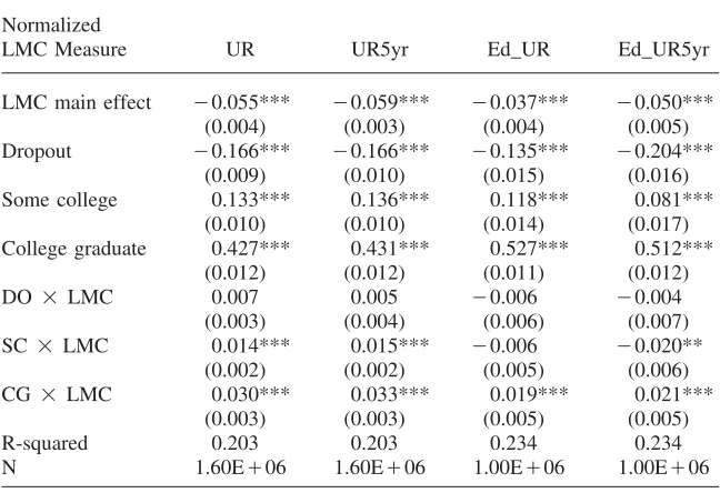
The results are somewhat different in Panel B, which uses the unemployment rate measures. The main effect is significant and large in all specifications. The estimates indicate average wage declines of 3.5 to 6 percent for high school graduates expe-riencing a standard deviation increase in state unemployment rates when they entered the labor market. College-educated workers are partially insulated from these effects, with college graduates only experiencing about half the wage impact of high school graduates.
Table 5(continued)
Panel B
Unemployment Rate Measures of Birth State Labor Market Conditions
Normalized
LMC Measure UR UR5yr Ed_UR Ed_UR5yr
LMC main effect ⳮ0.055*** (0.004)
R-squared 0.203 0.203 0.234 0.234
N 1.60EⳭ06 1.60EⳭ06 1.00EⳭ06 1.00EⳭ06
Notes: Dependent variable is log hourly wages. Data are taken from IPUMS versions of U.S. Census 5 percent samples for 1980, 1990, and 2000. Sample is noninstitutionalized U.S. natives with 5–8 years of potential labor market experience and positive wages in the previous year.
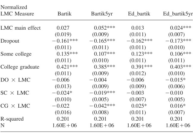
Table 5 shows that labor market entry conditions in a worker’s birth state have lasting medium-run wage effects but that generally these effects are tempered for college-educated workers and for college graduates in particular. Given the results in earlier tables, however, we know that more-educated workers—college graduates in particular—are less likely than other workers to stay in their birth states when labor market conditions there are poor. This might cause our estimates of the wage impacts of entry LMCs to be more attenuated for college graduates than for other groups. To address this, I created averages of state labor market conditions in a worker’s entry year weighted by historical migration patterns between the worker’s birth state and all other states. For an individual in education groupeborn in state s, I apply weightswjesto statej’sLMC measure that equal the education group long
Table 6
Wage Equation Estimates Using Migration Flow Weighted Average LMC Measures
Panel A
Weighted Average of State Bartik Measures
Normalized
LMC Measure Bartik Bartik5yr Ed_bartik Ed_bartik5yr
LMC main effect 0.027
R-squared 0.201 0.201 0.201 0.201
N 1.60EⳭ06 1.60EⳭ06 1.60EⳭ06 1.60EⳭ06
(continued)
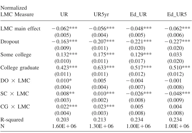
Results from using the weighted LMC measures in the wage equation are shown in Table 6. The main effects are generally larger using the weighted measures. This is consistent with a role for measurement error in attenuating the Table 5 coefficients. Estimates using the five-year Bartik measures imply medium-run average wage im-pacts of 2–5 percent for high school graduates following a standard deviation in-crease in entry labor market conditions. College graduates are insulated from the wage impacts of Bartik5yr conditions but not those inEd_bartik5yr. The Panel B estimates show wage impacts of 5–6 percent for high school graduates following a standard deviation change in entry unemployment rates.29College-educated workers are less insulated from the main effects of the weighted UR andUR5yr than the unweighted measures, and they are not insulated at all from the main effects of
Table 6(continued)
Panel B
Weighted Average of State Unemployment Rates
Normalized
LMC Measure UR UR5yr Ed_UR Ed_UR5
LMC main effect ⳮ0.062*** (0.005)
R-squared 0.203 0.213 0.234 0.234
N 1.60EⳭ06 1.30EⳭ06 1.00EⳭ06 1.00EⳭ06
Notes: Dependent variable is log hourly wages. Data are taken from IPUMS versions of U.S. Census 5 percent samples for 1980, 1990, and 2000. Sample is noninstitutionalized U.S. natives with 5–8 years of potential labor market experience and positive wages in the previous year. Weighting procedure applied to LMC measures described in text.
weightedEd_URorEd_UR5yr. They may even experience larger wage impacts of these conditions than their less-educated peers.30
The wage impacts in Table 6 can also be examined in relation to the migration choices in Tables 4a and 4b. Tables 4a and 4b show how a worker’s decision to locate in a state varies with entry labor market conditions in that state—and with education—and Table 6 shows how the entry conditions a worker actually experi-ences affects his wage. Thus, the decisions in Tables 4a and 4b will have conse-quences for workers that are, broadly speaking, outlined in Table 6. The migration responses to and wage impacts of the education-specific measures follow a consistent pattern. College graduates, and in some cases college-educated workers more broadly, experience lasting wage impacts of education-specific entry conditions that
are as large or larger than those for high school graduates. College graduates, and again sometimes those with some college, are more responsive to these conditions in their location choices. For example, Table 6 shows larger wage impacts of the education-specific Bartik measures for college graduates, and Table 4a shows that college graduates are more responsive to these conditions in their location choice than any other group.
VI. Conclusion
In this paper, I examined whether college graduates are more re-sponsive to distant labor market opportunities. The analysis answered three main questions. Are the location choices of college graduates are more sensitive to local labor market conditions than those of their less-educated peers? If so, does their choice of local market have lasting effects on their wages? And finally, are the wage and location responses to local conditions driven by an individual’s current market conditions or do other markets have similar push/pull effects?
To answer these questions, I matched a sample of workers with 5–8 years of potential labor market experience spanning 30 birth year cohorts to several measures of the state level conditions they faced at labor market entry. I examined the effects of these conditions on an individual’s choice of local labor market (defined as the state I observed him in 5–8 years after labor market entry) using two models of location choice: a linear probability model of residence in one’s birth state and a McFadden-style conditional logit model of the choice over all 50 possible states. I measured state labor market conditions for a worker’s labor market entry cohort using an index based on changes in industry employment (the Bartik measures) and using state unemployment rates. I also constructed education group specific versions of these measures that are intended to measure conditions relevant to a particular worker more precisely.
I find that workers with some higher education are more likely than high school graduates to live in a state that had high labor demand around their time of labor market entry in almost all specifications. This differential is generally largest for college graduates and in specifications using education-specific measures of state labor market conditions. I then examine whether a worker’s predicted entry condi-tions affect his wages 5–8 years later and whether this impact differs with education. Here the findings are more sensitive to the particular measure of entry labor market conditions. The medium-run wages of college-educated workers—graduates in par-ticular—are relatively unaffected by entry conditions measured using the average Bartik and unemployment rate measures. On the other hand, college graduates ex-perience medium-run wage impacts that are as large or larger than those for high school graduates when conditions are measured in an education-specific manner.
labor market conditions are larger when conditions are based on state of residence predicted from historical migration flows rather than birth state alone.
Is the pattern of wage and migration changes explored here consistent with an important role for inter-state arbitrage in setting the wages of young labor market entrants? When state labor market conditions are measured in an education-specific manner, the answer appears to be no. Improvements in conditions by these measures raise the relative labor supply of college graduates to a state and are accompanied by stable orincreasingrelative wages for college graduates. This is not consistent with an important role for arbitrage migration in wage setting for college graduates. Instead, it suggests that college graduates are more likely to move to take advantage of implicit contracts that lead to significantly higher wages for them over the dium-run. Their higher base levels of pay, along with potentially longer-lasting me-dium-run impacts of entry conditions for them, make college graduates more sen-sitive to entry labor market conditions when choosing a state of residence. On the other hand, when measures of average conditions are used, the corresponding relative wage and supply changes in these specifications are consistent with published esti-mates of the elasticity of substitution between more and less-skilled workers, sug-gesting that location choices arbitrage spatial wage differentials.31
Measurement error—in the sense that our approximations of experienced labor market conditions are inexact and may correspond differentially to conditions faced by different education groups—is likely driving this apparent discrepancy in the results. First, from comparing the measured impacts of entry conditions on wages across Tables 5 and 6, it is obvious that the conditions a worker actually experienced are stronger determinants of wages in the medium run. Because the education-spe-cific measures more accurately reflect conditions that a worker experienced, smaller responses to the average measures is likely explained by attenuation due to mea-surement error. This seems to be the case with the unemployment rate measures. With the Bartik measures, the average measure may be a better approximation of the market for less-educated workers while the education-specific measure better captures the market for more-educated workers.
Ultimately, I conclude that more-educated workers—college graduates in partic-ular—are more sensitive to local labor market conditions in choosing a state of residence. This is accompanied by larger absolute and possibly relative medium run wage impacts of these conditions, a finding that potentially explains the greater responsiveness of college graduates to distant opportunities. This result hinges on using particular measures of local labor market conditions that are tailored to dif-ferent education groups. This underscores the need to have a better understanding of what different measures of economic conditions actually represent, potentially an important question for future research. At the very least, it suggests that the use of a variety of measures is particularly useful when examining differential impacts of these conditions across skill groups.
References
Bartik, Timothy. 1991.Who Benefits from State and Local Economic Development Policies? Kalamazoo, Mich.: W.E. Upjohn Institute for Employment Research.
Bender, Stefan, and Till von Wachter. 2006. “In the Right Place at the Wrong Time: The Role of Firms and Luck in Young Workers’ Careers.”American Economic Review96(5): 1706–19.
Beaudry, Paul, and John DiNardo, John. 1991. “The Effect of Implicit Contracts on the Movement of Wages over the Business Cycle: Evidence From Micro Data.” Journal of Political Economy99(4):665–88.
Black, Dan, Terra McKinnish, and Seth Sanders. 2005. “The Economic Impact of the Coal Boom and Bust.”Economic Journal115(502):449–76.
Blanchard, Olivier, and Lawrence Katz. 1992. “Regional Evolutions.”Brookings Papers on Economic Activity1992(1):1–75.
Bonin, Holger, and Hilmar Schneider. 2004. “Analytical Prediction of Transitions Probabilities in the Conditional Logit Model.”IZA Discussion Paper #1015.
———. 2006. “Analytical Prediction of Transition Probabilities in the Conditional Logit Model.”Economics Letters90(1):102–107.
Bound, John, and Harry J. Holzer. 2000. “Demand Shifts, Population Adjustments, and Labor Market Outcomes during the 1980s.”Journal of Labor Economics18(1):20–53. Davies, Paul S., Michael J. Greenwood, and Haizheng Li. 2001. “A Conditional Logit
Approach to State to State Migration.”Journal of Regional Science41(2):337–60. Devereux, Paul J. 2002. “The Importance of Obtaining a High Paying Job.” Los Angeles:
University of California at Los Angeles, Department of Economics. Unpublished. Ellwood, David T. 1982. “Teenage Unemployment: Permanent Scars or Temporary
Blemishes?” InThe Youth Labor Market Problem: Its Nature, Causes, and Consequences, ed. Richard B. Freeman and David A. Wise. Chicago: University of Chicago Press.
Foote, Christopher, and Matthew Kahn. 2003. “Are Recessions Reallocations? Evidence from the Migration of U.S. Taxpayers, 1975–1998.” Medford, Mass.: Tufts University. Unpublished.
Gardecki, Rosella, and David Neumark. 1998. “Order from Chaos? The Effects of Early Labor Market Experiences on Adult Labor Market Outcomes.”Industrial and Labor Relations Review59(2):299–322.
Gelbach, Jonah. 2004. “Migration, the Lifecycle, and State Benefits: How Low is the Bottom?”Journal of Political Economy112(5):1091–1130.
Genda, Yuji, Ayako Kondo, and Souichi Ohta. 2010. “Long-Term Effects of a Recession at Labor Market Entry in Japan and the United States.”Journal of Human Resources 45(1):157–96.
Gould, William. 2000. “Interpreting Logistic Regression in All Its Forms.”Stata Technical BulletinSTB-53.
Greenwood, Michael J. 1975. “Research on Internal Migration in the United States: A Survey.”Journal of Economic Literature13(2):397–433.
Greenwood, Michael J. 1997. “Internal Migration in Developed Countries.” InHandbook of Population and Family Economics,ed. Mark R. Rosenzweig and Oded Stark. New York: Elsevier Science.
Guvenen, Fatih. 2007. “Learning Your Earning: Are Labor Income Shocks Really Very Persistent?”American Economic Review97(3):687–712.
Hamermesh, Daniel S. 1993.Labor Demand. Princeton, N.J.: Princeton University Press. Harris, Milton, and Bengt Holmstrom. 1982. “A Theory of Wage Dynamics.”Review of
Kahn, Lisa Blau. 2008. “The Labor Market Consequences of Graduating College in a Bad Economy.” New Haven, Conn.: Yale University. Unpublished.
Kennan, John, and James Walker. 2008. “The Effect of Expected Income on Migration Decisions.” Madison: University of Wisconsin-Madison. Unpublished.
Kletzer, Lori, and Robert Fairlie. 2003. “The Long Term Costs of Job Displacement for Young Adult Workers.”Industrial and Labor Relations Review56(4):682–98.
Knapp, Thomas A., Nancy E. White, and David E. Clark. 2001. “A Nested Logit Approach to Household Mobility.”Journal of Regional Science41(1):1–22.
Kydland, Finn. 1984. “Business Cycles and Aggregate Labor Market Fluctuations.”Federal Reserve Bank of Cleveland Working Paper #9312.
Malamud, Ofer, and Abigail Wozniak. 2008. “The Impact of College Graduation on Geographic Mobility: Identifying Education Using Multiple Components of Vietnam Draft Risk.”IZA Discussion Paper #3432.
McFadden, Daniel. 1974. “Analysis of Qualitative Choice Behavior.” InFrontiers in Econometrics, ed. Paul Zarembka. New York: Academic Press.
Meyer, Bruce. 2000. “Do the Poor Move to Receive Higher Welfare Benefits?” Chicago: University of Chicago. Unpublished.
O’Keefe, Suzanne. 2004. “Locational Choice of AFDC Recipients within California: A Conditional Logit Analysis.”Journal of Public Economics, 88(7–8):1521–42.
Oreopoulos, Philip, Till von Wachter, and Andrew Heisz. 2006. “Permanent and Transitory Effects from Graduating in a Recession.”NBER Working Paper #12159.
Oyer, Paul. 2006. “Initial Labor Market Conditions and Long-Term Outcomes for Economists.”Journal of Economic Perspectives20(3):143–60.
Ruggles, Steven and Matthew Sobek et al. 2003. Integrated Public Use of Microdata Series: Version 3.0. Minneapolis: Historical Census Projects, University of Minnesota, 2003. URL: http://www.ipums.org.
Saks, Raven E. 2008. “Job Creation and Housing Construction: Constraints on Metropolitan Area Employment Growth.” (Board of Governors Finance and Economics Discussion Paper Series #2005–49)Journal of Urban Economics64 (1):178–95
Solon, Gary, Robert Barsky, and Jonathan A. Parker. 1994. “Measuring the Cyclicality of Real
Wages: How Important is Composition Bias?”Quarterly Journal of Economics109(1):1– 25.
Topel, Robert H. 1986. “Local Labor Markets.”Journal of Political Economy94(3), Part 2: S111–S143.
———. 1994. “Regional Labor Markets and the Determinants of Wage Inequality.” American Economic Review84(2):17–22.
U.S. Census Bureau. 2003. “State-to-State Migration Flows: 1995 to 2000.” Census 2000 Special Reports (August).
URL: http://www.census.gov/population/www/cen2000/migration.html.
Ziliak, James P., Beth A. Wilson, and Joe A. Stone. 1999. “Spatial Dynamics and Heterogeneity in the Cyclicality of Real Wages.”Review of Economics and Statistics