Analiza in simulacija piramidnega lijaka

UNIVERSITY OF MARIBOR FACULTY OF ELECTRICAL ENGINEERING AND COMPUTER SCIENCE. Matija Drgestin. ANALYSIS AND SIMULATION OF PYRAMIDAL HORN ANTENNA Master’s thesis. Maribor, May 2019.

UNIVERSITY OF MARIBOR FACULTY OF ELECTRICAL ENGINEERING AND COMPUTER SCIENCE. Matija Drgestin. ANALYSIS AND SIMULATION OF PYRAMIDAL HORN ANTENNA Master’s thesis. Maribor, May 2019.

ANALIZA IN SIMULACIJA PIRAMIDNEGA LIJAKA Magistrsko delo. ANALYSIS AND SIMULATION OF PYRAMIDAL HORN ANTENNA Master’s thesis. Student:. Matija Drgestin. Study Programme:. Master’s Study Programme of Electrical Engineering. Study Field:. Telecommunications. Mentor:. doc. dr. Boštjan Vlaovič, univ. dipl. inž. el.. Lector:. prof. Marija Krznarić.

Thank you! I would like to express my deepest gratitude to my mentor Assist. Prof. Dr. Boštjan Vlaovič for his advice, support, and guidance while writing this master’s thesis. In addition, I am very thankful to the lector Marija Krznarić for spending time proofreading this thesis.. Furthermore, I owe special thanks and gratitude to my mother, father, brothers and my friends for their support, encouragement and love throughout my student life, and life in general.. Matija Drgestin. i.

Analiza in simulacija piramidnega lijaka. Ključne besede: piramidni lijak, valovod, simulacija, HFSS, frekvenca. UDK:. 621.396.67.029.5(043.2). Povzetek. 1. Uvod V magistrski nalogi je opisan piramidni lijak, njegove dimenzije in parametri. Parametri antene so podrejeni predvideni uporabi. Ob demonstraciji lastnosti razširjanja elektromagnetnega valovanja v predavalnici in laboratoriju smo praviloma prostorsko omejeni. Ker želimo demonstracije praviloma izvajati v daljnem polju, smo izbrali anteno manjših dimenzij. V prvem delu naloge smo podali analitično metodo za izračun parametrov glede na željeno resonančno frekvenco in dimenzije antene. V matematičnem modelu smo najprej izbrali željeno vrednost dobitka antene in nato z uporabo iterativne analitične metode določili dimenzije antene. Izračunane dimenzije so bile uporabljene pri izdelavi 3D modela antene. Sledila je simulacija 3D modela antene s profesionalnim orodjem ANSYS HFSS z uporabo numerične metode končnih elementov. Numerično in grafično predstavimo več parametrov antene, med drugim: dobitek,. ii.

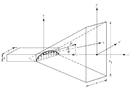
smernost, valovitost in sevalni diagram. V okviru simulacije smo preverili vpliv odstopanja dimenzij antene na parametre antene. Predstaviti smo želeli v kolikšni meri odstopanja vplivajo na posamezne parametre antene in na kaj je potrebno biti pozoren pri samogradnji. Kot referenčno smo uporabili anteno z analitično izračunanimi dimenzijami, ki je napajana neposredno preko valovoda. Pri praktični anteni smo uporabili anteno, ki je napajana preko koaksialnega kabla in SMA konektorja. Pridobljeni rezultati so predstavljeni in komentirani.. 2. Elektromagnetni valovi in valovod V teoretičnem delu so predstavljene osnove elektromagnetne teorije, ki so potrebne za analitičen opis piramidnega lijaka. Antena pretvarja elektromagnetno energijo v prostorski elektromagnetni val (sevanje) in obratno. Elektromagnetno valovanje je sestavljeno iz električnega in magnetnega polja, ki sta pravokotna med sabo in na smer širjenja valov – potujoče transverzalno valovanje. Za primer smo podali polvalni dipol, osnovno anteno, ki odlično predstavlja elektromagnetno sevanje. Skladno s teorijo elektromagnetnega valovanja, ki jo podajajo Maxwellove enačbe, sprememba električnega polja povzroča spremembo magnetnega polja in obratno. Elektromagnetni valovi vsebujejo določene lastnosti, specifične samo za to vrsto valov. Na svoji poti valovi pogosto naletijo na različne ovire, zato v nalogi predstavimo pojave, kot so interferenca, odboj in lom. Nekateri od teh pojavov so ključni za dojemanje razširjanja elektromagnetnih valov v zaprtih strukturah kot je valovod. Valovod je votla, prevodna, praviloma kovinska, struktura, ki se uporablja za učinkovit prenos elektromagnete energije. Uporabili smo pravokotni valovod, ki je primeren za uporabo pri višjih frekvencah in za napajanje piramidnega lijaka. Podane so dimenzije valovoda, katere se bodo uporabile za izračun dimenzij antene. Navedene dimenzije predstavljajo širino in višino valovoda, kjer je širina označena kot a in znaša 28,4988 mm, b pa je označena kot višina valovoda in znaša 12,6238 mm. V tem poglavju, smo tudi želeli izračunati t.i. mejno frekvenco, pod katero valovod ne more delovati. Poleg tega so bile opisane komponente električnega in magnetnega polja v valovodu.. iii.

Komponente polja so bile podane z enačbami ((3.7) - (3.12)), ki so razdeljene na vzdolžne in prečne komponente. Na koncu je bila grafično predstavljena distribucija polj vzdolž valovoda.. 3. Matematični model Matematični model antene je podan analitično. Izhodišče za izračun predstavljata resonančna frekvenca in dobitek antene. Oboje smo določili glede na željene dimenzije antene. Uporabljena je bila iterativna metoda v kateri smo želeli zadostiti enačbi (5.1) iz poglavja 5.3, pa tudi 5.6. Sledil je izračun dimenzije antene: višina, širina in dolžina stranic. Ob tem smo bili pozorni na možnost fizične izdelave antene v samogradnji. V primeru referenčne antene dimenzije antene so bile večje kot v primeru praktične antene, zato ker smo pri referenčni anteni uporabili večji dobitek, ki je znašal 19,7 dB. Izračunane vrednosti dimenzij praktične antene (poglavje 5.6) so podrejene demonstraciji na kratki razdalji, zato manjši dobitek antene ni problematičen. Izračunane dimenzije antene, so bile uporabljene v procesu simulacije. Rezultati simulacije so predstavljeni v poglavjih 5.4 in 5.8.. 4. Simulacija antene Izdelavo 3D modela antene in simulacijo smo izvedli z uporabo programskega okolja ANSYS Electromagnetic Suite 18, ki se uporablja za modeliranje različnih prenosnih struktur, anten, RF komponent in podobnih sklopov. Omogoča vizualizacijo elektromagnetnih polj v strukturi 3D modelov in okolici. Pridobljeni parametri antene so dobra preverba načrtovane izvedbe antene. Podrobneje smo preverili kako spremembe dimenzij antene vplivajo na rezultate izbranih parametrov antene. Tako smo določili dovoljeno odstopanje dimenzij izvedene antene glede na referenčno anteno. V poglavjih 5.3 in 5.7 je predstavljen potek simulacije in izdelava 3D modela referenčne in praktične antene. V teh poglavjih so podrobno opisovani koraki, ki so privedli do končnega izida, 3D modela antene. V simulaciji so uporabljene dimenzije, ki smo jih pridobili z analitično metodo. Razlika med referenčno in praktično anteno je v načinu napajanja; pri iv.

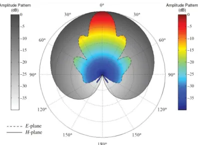
referenčni anteni je izvor elektromagnetnih valov bil valovod, med tem ko praktično anteno napajamo preko koaksialnega kabla in konektorja SMA. Pri praktični anteni se na parametrih pozna vpliv konektorja, ki vpliva na spremembo strukture valovoda antene.. 5. Rezultati Rezultate smo predstavili tako v tabelarični obliki kot z uporabo 2D grafov in 3D vizualizacij. Ob simulaciji smo izbrali željeno frekvenco ter preverili smernost, dobitek, porazdelitev električnega in magnetnega polja v anteni, razmerje stoječega valovanja in ostale parametre. Parametre piramidnega lijaka smo predstavili tudi grafično. Simulacija je potrdila pričakovane rezultate za oba modela antene. V obeh primerih so vrednosti pridobljenih parametrov v pričakovanih mejah, na primer, razmerje stoječega valovanja je pod 2, večina energije se izseva. Sevalni diagram smo predstavili v tridimenzionalnem prostoru. Iz slike je razvidno, da antena seva v predvidenem območju. Glavni snop in stranski snopi imajo pričakovano obliko. Nekatere parametre smo predstavili tudi dvodimenzionalno v E-ravnini in H-ravnini, saj se tako lažje odčitajo sevalni koti. Na koncentričnih krogih je predstavljen željen parameter, na primer, dobitek, ki se praviloma predstavlja v normirani logaritmični obliki.. 6. Sklep Osnovni namen naloge je predstavitev in opis piramidnega lijaka. V zaključku povzamemo celotno nalogo, od raziskovalnega in teoretičnega ozadja, analitičnega izračuna, tvorbe 3D modela, simulacije ter predstavitve in analize rezultatov. Po predstavitvi osnov teorije razširjanja elektromagnetnega valovanja in analitičnega opisa izbrane antene, smo dimenzije antene določili z matematičnim izračunom. Nato smo izdelali 3D model za referenčno in praktično anteno. Rezultati simulacije za referenčno anteno so bili skladni z matematičnimi napovedmi, kar je potrditev dobrega modela antene. Sledila je vrsta simulacij kjer smo preverili parametre anten ter njihovo odstopanje v primeru napak pri izdelavi zaradi odstopanja dimenzij antene. v.

Izbrane dimenzije smo spreminjali v območju od +10 mm do -10 mm, v korakih po 1 mm. Rezultati simulacije so pokazali vplive na parametre antene, naš cilj pa je bilo preveriti potrebno natančnost pri izdelavi tovrstne antene. Simulacije so potrdila pričakovanja in pokazale, da nenatančnost pri izdelavi antene ne bo bistveno vplivala na delovanje v predvidenem sistemu.. vi.

Analysis and simulation of pyramidal horn antenna. Key words: pyramidal horn, waveguide, simulation, HFSS, frequency. UDK:. 621.396.67.029.5(043.2). Abstract. This master's thesis describes a pyramidal horn antenna, its dimensions and parameters. The antenna parameters are submitted to the intended use. When demonstrating the properties of the electromagnetic wave propagation in the laboratory, we are generally spatially limited. In order to carry out antenna demonstrations in the far field, an antenna of smaller dimensions has been chosen. In the first part of the thesis, an analytical method for calculating the parameters according to the desired resonant frequency and the dimensions of the antenna has been presented. In the mathematical model, the desired gain value of the antenna was selected and then the dimensions of the antenna, using an iterative analytical method, was determined. The calculated dimensions were used in the design of the 3D model antenna. The simulation of the 3D model antenna was carried out by the professional tool ANSYS HFSS which uses a numerical method with a finite number of elements. Numerically and graphically, we present several parameters of the antenna, including gain, direction, standing wave ratio and radiation diagram. In the simulation, the influence of the deviation of the antenna dimensions on the parameters of vii.

the antenna was examined. The objective was to present to what extent the deviations influence the individual parameters of the antenna and what needs to be considered, while planning the physical realization of the antenna. As a reference, we used an antenna with analytically calculated dimensions, which is fed directly through the waveguide. In practical terms, an antenna was fed via a coaxial cable and a SMA connector. The obtained results are presented and commented.. viii.

Table of Contents 1. INTRODUCTION ............................................................................................................................ 1 2. ELECTROMAGNETIC WAVE .......................................................................................................... 3 2.1 Properties and occurrences of electromagnetic waves ....................................................... 5 2.2 Electromagnetic spectrum................................................................................................... 11 2.3 Maxwell’s equations ............................................................................................................ 12 2.3.1 First Maxwell’s equation............................................................................................... 13 2.3.2 Second Maxwell’s equation.......................................................................................... 13 2.3.3 Third Maxwell’s equation ............................................................................................. 14 2.3.4 Fourth Maxwell’s equation........................................................................................... 15 3. WAVEGUIDES .............................................................................................................................. 16 3.1 Rectangular waveguides ...................................................................................................... 18 3.2 Transverse modes ................................................................................................................ 19 3.3 Dominant mode TE10. Cut-off frequency of the WR-112 ................................................... 21 3.4 Electric and magnetic fields in the waveguide. Maxwell’s equations ............................... 25 4. ANTENNAS .................................................................................................................................. 29 4.1 Antenna parameters ............................................................................................................ 30 4.1.1 Radiation pattern. Beamwidth ..................................................................................... 31 4.1.2 Field regions .................................................................................................................. 33 4.1.3 Polarization.................................................................................................................... 35 4.1.4 Power density................................................................................................................ 37 4.1.5 Directivity and antenna gain. Radiation intensity ....................................................... 39. ix.

4.2 Types of antennas ................................................................................................................ 41 4.2.1 Monopole antennas...................................................................................................... 41 4.2.2 Dipole antennas ............................................................................................................ 42 4.2.3 Aperture antennas ........................................................................................................ 44 4.3 E-plane horn antenna .......................................................................................................... 47 4.3.1 Geometry and parameters ........................................................................................... 47 4.3.2 Aperture field distribution and far-field region. Directivity ........................................ 50 4.3.3 Optimum antenna dimensions..................................................................................... 54 4.4 H-plane horn antenna .......................................................................................................... 55 4.4.1 Geometry and dimensions ........................................................................................... 55 4.4.2 Aperture field distribution and far-field region. Directivity ........................................ 58 4.4.3 Optimum antenna values ............................................................................................. 61 4.5 Pyramidal horn antenna ...................................................................................................... 61 4.5.1 Geometry and dimensions ........................................................................................... 62 4.5.2 Aperture field distribution and far-field region. Directivity ........................................ 63 4.5.3 Optimum antenna values ............................................................................................. 65 5. ANTENNA SIMULATION .............................................................................................................. 66 5.1 Starting the HFSS simulator ................................................................................................. 66 5.2 Mathematical calculation of the reference pyramidal horn antenna ............................... 70 5.3 HFSS design procedure of the reference pyramidal horn antenna ................................... 73 5.4 Results of the reference pyramidal horn antenna ............................................................. 79 5.5 Deviations of the reference pyramidal horn antenna ........................................................ 89 5.6 Mathematical calculation of the practical pyramidal horn antenna ............................... 100. x.

5.7 HFSS design procedure of the practical pyramidal horn antenna ................................... 102 5.8 Results of the practical pyramidal horn antenna ............................................................. 105 6. CONCLUSION ............................................................................................................................ 112. xi.

Table of Figures Figure 1: Electric and magnetic field ............................................................................................... 3 Figure 2: Manifestation of EM radiation ......................................................................................... 4 Figure 3: Manifestation of EM radiation ......................................................................................... 5 Figure 4: Reflection........................................................................................................................... 6 Figure 5: Refraction .......................................................................................................................... 7 Figure 6: Total internal reflection .................................................................................................... 8 Figure 7: Diffraction .......................................................................................................................... 9 Figure 8: Constructive interference ............................................................................................... 10 Figure 9: Destructive interference ................................................................................................. 10 Figure 10: Electromagnetic spectrum ........................................................................................... 12 Figure 11: Waveguide..................................................................................................................... 16 Figure 12: Waveguide coupling ..................................................................................................... 17 Figure 13: Wave paths in the waveguide – top view .................................................................... 17 Figure 14: Geometry of rectangular waveguide in Cartesian coordinate system ...................... 18 Figure 15: WR-112 waveguide ....................................................................................................... 19 Figure 16: Comparison between TE and TM modes in rectangular waveguide ......................... 20 Figure 17: Waveguide WR-112 dimension specifications ............................................................ 23 Figure 18: Electric and magnetic field lines within a waveguide ................................................. 26 Figure 19: Transmitting antenna ................................................................................................... 29 Figure 20: Receiving antenna ......................................................................................................... 30 Figure 21: Antenna radiation pattern ............................................................................................ 32 Figure 22: Radiation patterns ........................................................................................................ 33 Figure 23: Field regions and field distribution .............................................................................. 34 Figure 24: Types of polarization..................................................................................................... 36 Figure 25: Graphical representation of Poynting's vector ........................................................... 38 Figure 26: Examples of monopole antennas ................................................................................. 42 xii.

Figure 27: Examples of dipole antennas ....................................................................................... 43 Figure 28: Examples of microwave antennas ............................................................................... 44 Figure 29: E-plane and H-plane antenna ....................................................................................... 46 Figure 30: Pyramidal horn antenna ............................................................................................... 46 Figure 31: Geometry of E-plane antenna ...................................................................................... 47 Figure 32: Cross-section of the E-plane horn antenna ................................................................. 48 Figure 33: Directivity as a function of aperture height ................................................................ 49 Figure 34: E-plane horn antenna patterns in E-plane and H-plane ............................................. 52 Figure 35: Table of Fresnel's integrals ........................................................................................... 54 Figure 36: Geometry of H-plane antenna ..................................................................................... 55 Figure 37: Cross-section of the H-plane horn antenna ................................................................ 56 Figure 38: Directivity as a function of aperture width .................................................................. 57 Figure 39: H-plane horn antenna patterns in E-plane and H-plane............................................. 60 Figure 40: Geometry of pyramidal horn antenna ......................................................................... 62 Figure 41: Top view (H-plane) of pyramidal horn ......................................................................... 62 Figure 42: Side view (E-plane) of pyramidal horn ......................................................................... 63 Figure 43: Pyramidal horn antenna pattern in E-plane and H-plane ........................................... 64 Figure 44: Electronics Desktop interface ...................................................................................... 66 Figure 45: Electronics Desktop toolbar ......................................................................................... 67 Figure 46: ANSYS HFSS window with associated parts ................................................................. 67 Figure 47: Project Manager window ............................................................................................. 68 Figure 48: Properties window ........................................................................................................ 68 Figure 49: Components Library window ....................................................................................... 69 Figure 50: 3D Modeler window ..................................................................................................... 69 Figure 51: Creating a waveguide ................................................................................................... 74 Figure 52: Waveguide values ......................................................................................................... 74 Figure 53: Horn aperture values .................................................................................................... 74 Figure 54: Waveguide and rectangle ............................................................................................. 75. xiii.

Figure 55: Waveguide face selection............................................................................................. 75 Figure 56: Pyramidal horn antenna ............................................................................................... 76 Figure 57: Antenna wall thickness ................................................................................................. 77 Figure 58: Selection of perfect conductor .................................................................................... 77 Figure 59: Region around horn antenna ....................................................................................... 78 Figure 60: Excitation port values ................................................................................................... 78 Figure 61: Assignment of excitation port ...................................................................................... 79 Figure 62: Frequency sweep .......................................................................................................... 80 Figure 63: Waveguide and reference antenna dimensions ......................................................... 81 Figure 64: Results of reference antenna parameters ................................................................... 81 Figure 65: Return Loss .................................................................................................................... 83 Figure 66: VSWR ............................................................................................................................. 84 Figure 67: Directivity ...................................................................................................................... 84 Figure 68: Gain ................................................................................................................................ 85 Figure 69: Total radiated electric field .......................................................................................... 86 Figure 70: Electric field strength .................................................................................................... 87 Figure 71: Magnetic field strength ................................................................................................ 87 Figure 72: Electric field in E-plane ................................................................................................. 88 Figure 73: Electric field in H-plane ................................................................................................. 89 Figure 74: Waveguide length ......................................................................................................... 90 Figure 75: Graphical representation of simulated parameters – waveguide length .................. 91 Figure 76: Waveguide width .......................................................................................................... 92 Figure 77: Graphical representation of simulated parameters – waveguide width ................... 93 Figure 78: Waveguide height ......................................................................................................... 94 Figure 79: Graphical representation of simulated parameters – waveguide height .................. 95 Figure 80: Aperture width .............................................................................................................. 96 Figure 81: Graphical representation of simulated parameters – aperture width ...................... 97 Figure 82: Aperture height ............................................................................................................. 98. xiv.

Figure 83: Graphical representation of simulated parameters – aperture height ..................... 99 Figure 84: Waveguide and practical antenna dimensions ......................................................... 102 Figure 85: Antenna parameters ................................................................................................... 102 Figure 86: Pyramidal horn antenna with SMA connector .......................................................... 103 Figure 87: Lumped port ................................................................................................................ 104 Figure 88: SMA connector............................................................................................................ 104 Figure 89: Return Loss .................................................................................................................. 106 Figure 90: VSWR ........................................................................................................................... 106 Figure 91: Directivity .................................................................................................................... 107 Figure 92: Gain .............................................................................................................................. 108 Figure 93: Total radiated electric field ........................................................................................ 108 Figure 94: Electric field in E- and H-plane ................................................................................... 109 Figure 95: Electric field strength .................................................................................................. 110 Figure 96: Magnetic field strength .............................................................................................. 110. xv.

List of abbreviations AC. Alternating Current. AM. Amplitude Modulation. dB. decibel. dBi. decibel (isotropic). EHF. Extremely High Frequency. ELF. Extremely Low Frequency. EM. Electromagnetic. FM. Frequency Modulation. FNBW. first-null beamwidth. GHz. Gigahertz. GPS. Global Positioning System. HEM. Hybrid Electromagnetic mode. HF. High Frequency. HPBW. half-power beamwidth. Hz. hertz. kHz. kilohertz. LF. Low frequency. MF. Medium frequency. MHz. Megahertz. mm. millimeter. PEC. Perfect Electric Conductor. PTFE. Polytetrafluoroethylene. SHF. Super high frequency. SLF. Super low frequency. SMA. SubMiniature version A. xvi.

TE. Transverse Electric mode. TEM. Transverse Electromagnetic mode. THF. Tremendously High Frequency. THz. Terahertz. TM. Transverse Magnetic mode. UHF. Ultra-high frequency. ULF. Ultra-low frequency. VHF. Very high frequency. VLF. Very low frequency. WLAN. Wireless Local Area Network. WR. Waveguide Rectangular. xvii.

1. INTRODUCTION Communications have become an unavoidable part of human life. In the past, it was difficult to imagine that the information can be transferred with high reliability and low latency from one end of the world to the other and in matter of seconds. Exchange of information is realized by different communication paths in which a certain data rate of information can be achieved in accordance with the frequency range and the standards specifically used by the certain communication technology. Information can be transferred by means of different technologies, such as optical fibers and copper cables but also through waveguides and antennas, which is known as radiocommunication. Radiocommunication falls into the area of electrical engineering, which uses radio waves as a media to transmit and receive information. Radio waves are electromagnetic waves arranged into a frequency range from 3 kHz to 300 GHz. Due to various properties and occurrences of the electromagnetic waves, frequency range of radio waves has been divided into twelve areas. Since radiocommunication development is the cause of widespread use in a variety of areas, it is necessary to allocate frequency ranges in exact areas to avoid interference and thus allowing a smooth operation of certain services [1, 2].. Purpose of this master's thesis is to undergo with a mathematical calculation of the pyramidal horn antenna and to determine its dimensions, perform the process of simulating the model of the antenna, and generate the values of the antenna parameters. Furthermore, it is necessary to alterate values of individual antenna dimensions in the given range, aiming to determine the deviations in relation to the original values. Deviations are important for determining the exact antenna dimension values at which the antenna still maintains its efficiency. The idea is to carry out an antenna calculation for the 9 GHz frequency band, with gain value above 15 dB, preferably. After the calculation is completed, an antenna simulation will be performed in which the individual antennas parameters such as gain, directivity, standing wave ratio, etc. will be generated through the simulation process. The antenna dimension values will be subjected to. 1.

changes, which will range from -10 mm to +10 mm, in steps of 1 mm, to see how the change of the antenna's dimensions will affect the change of the parameters. All the results will be displayed in table and graph forms. Further in the text, this will be considered as a reference pyramidal horn antenna.. Mentioned reference model is needed to create an antenna (later on, it is referred to as a practical antenna) that will be used for the purposes of calculating polarization losses within controlled conditions, in the lecture room or laboratory. Namely, the goal is to calculate the antenna for the same frequency band but with a lower gain as the reference antenna. Lower gain and therefore smaller antenna dimensions are needed to physically create two antennas in order to measure polarization losses. In addition, smaller dimensions are required, as the distance between the antennas is less than one meter.. Prior to the calculation, simulation and retrieval of antenna parameters, chapters will be discussed in this master’s thesis that are necessary to understand the practical part of the thesis. In essence, the electromagnetic waves, their properties and phenomena, as well as the Maxwell equations, which are necessary to represent and understand the nature of electromagnetic waves will be explained in following chapters. Furthermore, the waveguide will be described as a special type of narrow, electric conduit, which is required for electromagnetic waves to propagate towards the antenna aperture. For the purpose of this thesis, a rectangular waveguide is selected. In addition, the thesis will contain a chapter on antennas, their parameters and types. At the end, a conclusion regarding calculation and simulation process of the antenna, as well as representation of obtain values will be given.. 2.

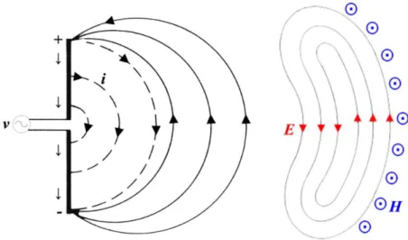
2. ELECTROMAGNETIC WAVE Electromagnetic radiation represents an electromagnetic wave that consists of electric and magnetic fields, which propagate (radiate) through free-space. An electric charge represents an electrically charged body in space. There is always an electrical field at the points of space around the electrical charge. The electric charge acts on all surrounding electrically charged bodies with an attracting or repulsive force, depending on the polarity of other charged bodies. This action of electrically charged bodies causes movement, resulting in the manifestation of a magnetic field. Essentially, electric field is the result of changing magnetic field, and magnetic field is the result of changing electric field. The process of mutual production of electric and magnetic fields results in the propagation of the electromagnetic waves through the space at a speed equal to the speed of light [3 (pp. 590-643), 4, 5, 6 (pp. 1-14)].. Figure 1: Electric and magnetic field. 3.

Figure 1 depicts above-mentioned fields that are mutually perpendicular to each other, as well as they are perpendicular to the direction of wave propagation. Therefore, electromagnetic wave is a transverse wave. Fields are illustrated in three-dimensional Cartesian coordinate system, where coordinates are denoted with letters 𝒙, 𝒚 and 𝒛.. Figure 2 and Figure 3 provide simplified presentation how electromagnetic radiation is being produced. A perfect example is a half-wavelength dipole antenna, which has two conducting rods, where each rod is 𝝀/𝟒 long. The rods are connected to the AC power source (denoted as 𝒗). The voltage generator induces an electric field (denoted as 𝑬), which causes force to the electric charge. Due to free electrons in the conducting media, an electric current (denoted as 𝒊) is generated, and it begins to flow, from the point of higher potential to the point of lower potential. As current flows, the electric charges are formed on the rods, where one side is positive, and the other is negative, as shown in Figure 2 [3 (pp. 590-643), 4, 5, 6 (pp. 1-14)].. Figure 2: Manifestation of EM radiation. Electric field produces magnetic field (denoted as 𝑯) and its direction is determined by the righthand rule. Since the half-wave dipole is connected to the alternating voltage generator, at some point the electric current will change direction, creating a shift in electric charges, i.e. the positive side of the rod will become negative, and negative one will become positive. By 4.

changing direction of the electric current, the direction of electric and magnetic field changes too, as shown in Figure 3. The electromagnetic field consists of two vector fields, E and H, that are interconnected [3 (pp. 590-643), 4, 5, 6 (pp. 1-14)].. Figure 3: Manifestation of EM radiation. 2.1 Properties and occurrences of electromagnetic waves Electromagnetic waves have four important properties:. 1. Unlike other (mechanical) waves that use media to propagate, electromagnetic waves are propagated by oscillation of electric and magnetic fields. In addition, electromagnetic wave can travel through vacuum.. 2. The direction of electric and magnetic fields within electromagnetic wave is perpendicular to one another, and both of them are perpendicular to the direction of wave propagation, making them transverse waves.. 3. In electromagnetic wave, oscillating electric and magnetic fields are in phase.. 5.

4. The velocity of electromagnetic waves depends only on the electric and magnetic properties of the media in which they propagate. Electromagnetic waves travel at the speed of light – 𝒄 =. 1 √𝜀0 ∙𝜇0. 𝑚. ≈ 2.998 ∙ 108 [ 𝑠 ]. By propagating in free-space, electromagnetic waves can encounter on certain obstacles, which can result in various wave phenomena, such as reflection, refraction, interference, and diffraction.. Reflection is the wave occurrence, where propagating wave is reflected from the surface. The amount of wave, that is reflected, depends on the composite characteristics of the material or the surface from which the wave has been reflected. Figure 4 depicts a ray of light that falls on the smooth surface (mirror) at the angle of incidence, denoted as 𝜽𝒊 . The ray of light is reflected from the surface at the angle of reflection, denoted as 𝜽𝒓 . Figure 4 shows that the angle of incidence and the angle of reflection are equal, thus meeting the requirements for realizing the wave reflection. Normal represents the line, which divides mentioned angles into two equal parts. Normal is perpendicular to the surface [3 (pp. 644-678), 7, 8].. Figure 4: Reflection. 6.

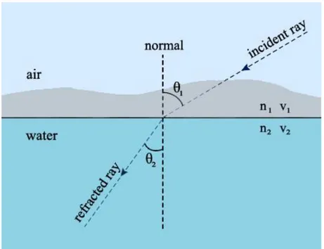
Refraction is one of the most important wave occurrence. The electromagnetic wave refracts as it passes from one (optically less dense) media to another (optically denser) media, due to velocity difference of the propagated wave in different media. Change of velocity results in change of wave propagation. Refraction can be imagined as phenomenon, where ray of light bends when it passes from one media to another – Figure 5. Snell’s law describes refraction. sin θ1 𝑣1 𝑛2 = = sin θ2 𝑣2 𝑛1. (2.1). where: θ1 – angle of incidence θ2 − angle of refraction 𝑣1 , 𝑣2 – wave velocities 𝑛1 − refraction index of optically less dense media 𝑛2 − refraction index of optically denser media. Figure 5: Refraction. 7.

In the example, where ray of light passes from optically denser media into an optically less dense media, a total internal reflection occurs (Figure 6). More precisely, total internal reflection occurs, when the angle of incidence is greater than the critical angle – 𝜽𝒄 . The critical angle represents the angle, where the ray of light is no longer refracted but totally reflected, due to passing through a denser media to a less dense media. The formula for determining the critical angle is expressed as follows 𝑛2 θc = sin−1 ( ) 𝑛1 Figure 6 depicts the angles of incident waves. Angles that are smaller than the critical angle cause refraction of the ray of light at the boundary of the two media. Furthermore, incident wave angles, that are greater than the critical angle, result in total internal reflection, where incident wave reflects from the boundary of the two media back to the optically denser media. Finally, incident wave angle, equal to the critical angle, causes the wave travel along the boundary of the two media [3 (pp. 644-678), 7, 8, 9, 10].. Figure 6: Total internal reflection. 8.

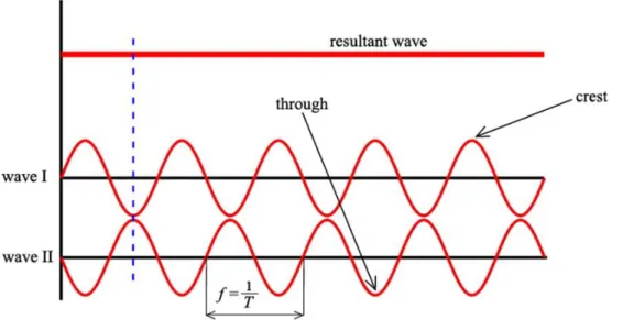
Diffraction is a physical phenomenon that occurs when wave turns its motion behind the edge of the barrier which the waves encounter. If the waves encounter a barrier whose dimensions are approximate to the length of the wave, diffraction will cause the interference in the waves. In Figure 7, it is apparent that a greater obstacle opening results in less wave spread than a smaller obstacle opening. Essentially, diffraction describes the wave behaviour after the wave passes through the narrow opening or bypasses a certain obstacle [3 (pp- 679-712), 7, 8].. Figure 7: Diffraction. Interference is wave occurrence that describes an interaction between two or more waves, which occurs at the same place and time. Interference is easily represented by the example of periodic waves. The periodic wave is a wave, which repeats itself after a certain period of time. Elements that describe periodic waves are frequency (𝒇) or wavelength (𝝀), period (𝑻), and amplitude (𝑨). Figure 8 depicts two sine waves that are aligned precisely, meaning that they are in phase. The sum of their amplitudes will result in a resultant wave, which has twice the amplitude of the initial two sine waves. This type of interference is called constructive interference. As seen in Figure 8, crests are aligned with crests, and throughs are aligned with throughs [3 (pp. 679-712), 11, 12].. 9.

Figure 8: Constructive interference. Figure 9 depicts two sine waves that are out of phase or phase-shifted. This shift causes a crest of one sine wave to coincide with the through of another sine wave. Thus, their amplitudes are cancelled, and the resultant wave amplitude is equal to zero. This is an example of destructive interference [3 (pp. 679-712), 11, 12].. Figure 9: Destructive interference. 10.

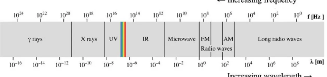
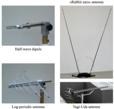
2.2 Electromagnetic spectrum Electromagnetic radiation can be found on different frequencies and wavelengths. Frequency or wavelength ranges are referred to as spectrum. Electromagnetic spectrum represents the strength of electromagnetic radiation as the function of frequency or wavelength. Spectrum contains different frequency ranges and applications in various areas. ITU is a United Nations regulatory body that regulates, coordinates and monitors the use of frequency domains globally. The ITU has defined twelve frequency ranges within the radio spectrum [13, 14].. Frequency range between 3 Hz and 3 kHz (ELF, SLF, and ULF) is used in underwater communications and mining, due to long wavelengths that can penetrate under water or even earth. Ground dipole antenna and various types of coils and ferrite loop antennas are used in these frequency ranges [13, 14].. Various services use frequencies between 3 kHz and 3 MHz (VLF, LF, and MF), such as radiolocation, government and military services, long distance communications, aviation, radio amateurism and AM radio broadcasting. Large vertical monopole antennas are used in these ranges [13, 14].. Between the 3 MHz and 3 GHz range HF, VHF, and UHF frequencies are placed. These frequencies are used in radio amateurism, television broadcasting, aircraft and aviation communications, WLAN, GPS, Bluetooth, FM radio broadcasting, satellite radio, and many more. Most commonly used antennas are Yagi-Uda dipole antenna, reflector antenna, small monopole and helix antennas, and array antenna systems, such as reflective antenna and collinear antenna [13, 14].. The final frequency set consists of SHF, EHF, and THF frequencies, placed between 3 GHz and 3 THz frequency range. Astronomy, microwave communications, radar, satellites, point-to-point. 11.

communication and X-rays are some of the applications used within this range. This frequency range, especially super high frequency range (3 GHz – 30 GHz) is important for this thesis, because of the small wavelength, that allows microwaves to be precisely directed into narrow beams by horn antenna. Horn antenna is a type of aperture antenna, which is used for frequencies above 300 MHz. It is characterized by low loss, high gain, moderate directivity, and is relatively easy to design and build. Horn antenna will be explained in detail in the following chapters. Frequency and wavelength ranges are shown in Figure 2.10 [13, 14].. Figure 10: Electromagnetic spectrum. 2.3 Maxwell’s equations In the late 19th century, a Scottish scientist James Clerk Maxwell developed the theory of electromagnetic fields. Previously established laws, such as Ampère’s and Gauss’s law as well as Faraday’s law of induction, guided him. With all gathered knowledge, he set four main equations that describe the unified theory of the electric and magnetic fields on charges and currents, as well as their interaction, which occurs when the fields change in time. According to those equations, changes in the electric field cause changes in the magnetic field and vice versa [3 (pp. 623-645), 15].. 12.

2.3.1 First Maxwell’s equation First Maxwell’s equation (2.2) is interpreted as Gauss’s law for electric fields. Left side of expression describes electric field lines as open curve. These electric field lines begin on the positive electric charge, and terminate on the negative electric charge. The right side of the expression states that electric flux through any closed surface is equal to the sum of all the electric charges contained within closed surface. Essentially, electric flux through a closed surface that does not contain any electric charge is equal to zero → the source of an electric field is an electric charge [3 (pp. 623-645), 6 (p. 193), 15 (pp. 1-38)].. ⃗ ∙ 𝑑𝑺 = ∮𝑬. ∑ 𝑸𝒕𝒐𝒕𝒂𝒍 𝜺. (2.2). where: V 𝐸⃗ – electric field strength [m]. 𝑑 − differential 𝑆 – closed surface [m2 ] 𝑄𝑡𝑜𝑡𝑎𝑙 – sum of electric charges within closed surface [C] F. 𝜀 – dielectric permittivity; ε = εr ∙ ε0 = 8.854 ∙ 10−12 [m], εr = 1 (free-space). 2.3.2 Second Maxwell’s equation According to this law, there are no magnetic monopoles existing in nature → magnetic field has a source, but there are no magnetic charges. In this case, a magnetic field lines are closed, which means that magnetic flux through a closed surface is equal to zero. There is a link between the first and second Maxwell equation (2.3), regarding the (integral) form of equation, but they differ in content and interpretation [3 (pp. 623-645), 6 (p. 193), 15 (pp. 43-55)].. 13.

⃗⃗ ∙ 𝑑𝑺 = 0 ∮𝑩. (2.3). where: ⃗ − magnetic field strength [ A ] 𝐵 m 𝑆 – closed surface [m2 ]. 2.3.3 Third Maxwell’s equation Third Maxwell’s equation (2.4) states that any change in electric field creates a change in the magnetic field. That was explained well in Faraday’s law of induction, which states that the line integral of the electric field along the closed surface is equal to negative value of the magnetic flux through the closed surface. A negative sign indicates that induced electric field opposes the change of the magnetic flux [3 (pp. 623-645), 6 (p. 193), 15 (pp. 58-80)].. ∮ ⃗𝑬 ∙ 𝑑𝒍 = −. 𝑑 ⃗ ∙ 𝑑𝑺 ∙ ∫ ⃗𝑩 𝑑𝑡. (2.4). where: V 𝐸⃗ – electric field strength [m]. 𝑑𝑙 − line integral of electric field 𝑆 – closed surface [m2 ] 𝑑 − differential 𝑡 − time [s] ⃗ − magnetic field strength [ A ] 𝐵 m. 14.

2.3.4 Fourth Maxwell’s equation Fourth Maxwell’s equation (2.5) is explained by Ampère's law. Ampère's law is a physical law that states: magnetic field is generated because of electric charge movement, thus connecting electric and magnetic occurrences. From the integral standpoint, it states that the line integral of magnetic field along closed loop is proportional to the total electric current, penetrating open surface enclosed by the loop. Essentially, the source of magnetic field is the electric current. This equation is expressed as [3 (pp. 623-645), 6 (p. 193), 15 (pp. 83-108)]. ⃗⃗ ∙ 𝑑𝒍 = 𝜇 ∙ ( 𝑱 + 𝜀 ∙ ∮𝑩. 𝑑 ⃗ ∙ 𝑑𝑺 ) ∙ ∫𝑬 𝑑𝑡. (2.5). where: ⃗ − magnetic field strength [ A ] 𝐵 m 𝑑𝑙 − line integral of magnetic field 𝑆 – open surface [m2 ] H. 𝜇 − magnetic permeability; μ = μr ∙ μ0 = 4π ∙ 10−7 [m], μr = 1 (free-space) A. 𝐽 − electric current density [m2 ] F. 𝜀 – dielectric permittivity; ε = εr ∙ ε0 = 8.854 ∙ 10−12 [m], εr = 1 (free-space) 𝑑 − differential V 𝐸⃗ – electric field strength [m]. 15.

3. WAVEGUIDES Waveguide is constructed as hollow, metal tube usually made of copper, aluminum, brass or even silver (Figure 11) that radiates electromagnetic waves from its conductive walls toward the antenna aperture and ultimately into the free-space. Electromagnetic waves propagate in a direction, which is defined by waveguide’s physical boundaries. There are different types of waveguides based on their cross-section, such as elliptical, circular and rectangular. Waveguide interior can be filled with dielectric, most commonly with air. Traveling waves within a waveguide are transmitted by total internal reflection, where incident wave impacts on a media boundary (inner walls of the waveguide) at an angle that is larger than a critical angle (see chapter 2.1).. Figure 11: Waveguide. Since the waveguide is a type of transmission media with small losses compared to the coaxial cable, it is ideal for wave propagation at frequencies above 3 GHz. Waveguides show lower attenuation properties and are more capable for high power energy transmission than coaxial cable. Waveguide uses small coupling elements, such as stubs (probes) or loops, to make the waves easier to insert into, and extract from the waveguide. Essentially, stubs or loops are used to generate waves into waveguide. These coupling elements come in form of a dipole (usually half-wave dipole) antenna, with 𝝀/𝟒 in physical length for stub coupling or as short wire loop for a loop coupling, that are embedded inside of the waveguide – Figure 12. 16.

Figure 12: Waveguide coupling. Probes or loops that are embedded inside the waveguide, generate waves into it. Waves within waveguide travel in zigzag pattern, and are successively reflected between the waveguide walls, due to the total reflection (depicted in Figure 13). As waves travel, they hit waveguide wall at some angle. The wave paths of these angles are larger at higher frequencies – Figure 13 a). As the operating frequency decreases, the path between the waves becomes shorter – Figure 13 b) and 13 c). At cut-off frequency, waves “jump” up and down between the walls of the waveguide, thus preventing the movement of energy forward – Figure 13 d) [18, 19].. Figure 13: Wave paths in the waveguide – top view. 17.

3.1 Rectangular waveguides Rectangular waveguide has rectangular cross-section, which is defined by sides 𝒂 and 𝒃, where 𝒂 represents width, and 𝒃 represents height of the waveguide, where 𝑎 > 𝑏. In addition, a hollow space within the waveguide is filled with electric permittivity, denoted as 𝜺 and magnetic permeability, denoted as 𝝁 (Figure 14). In Cartesian coordinate system on Figure 14, there are three dimensions: 𝒙 represents a waveguide width (denoted with letter 𝒂), 𝒚 represents a waveguide height (denoted with 𝒃) and 𝒛 represents a direction of wave propagation.. Figure 14: Geometry of rectangular waveguide in Cartesian coordinate system. Dimensions 𝒂 and 𝒃 are used to determine the range of operating frequency of the waveguide. WR is an abbreviation for Waveguide Rectangular, i.e. a type of standard that determines waveguide dimensions, operating frequency range and cut-off frequency for upper and lower operating mode. For this thesis, a WR-112 (Figure 15) has been chosen as waveguide, on which pyramidal horn will be mounted. WR-112 waveguide is designed for frequency range between 7.05 GHz and 10 GHz, with dimensions for side 𝒂 = 28.4988 mm and for side 𝒃 = 12.6238 mm [19, 20, 21].. 18.

Figure 15: WR-112 waveguide. 3.2 Transverse modes The propagation modes and the operating wavelength supported in the waveguide, depend on its dimensions. Generally, the waveguide works best only when one mode, the so-called dominant mode, is present. Each mode shows some special propagation properties, such as wave (information, signal) attenuation, phase shift of electromagnetic waves, and propagation speed. When the radiated energy of electromagnetic waves is propagated in multiple modes at the same time, the difference in propagation speed occurs, which leads to wave distortion. In order to eliminate this unwanted multimode effect, the cross-sectional dimensions of the waveguide must be selected in such a way that only one mode can be transmitted at given wavelength (frequency).. Mentioned modes are called transverse modes, and they can be divided into several groups: transverse electric – TE, transverse magnetic – TM, transverse electromagnetic – TEM and hybrid – HEM. In TE mode (Figure 16), there is a magnetic field component in the direction of propagation, but not electric, since it is perpendicular (transverse) to the direction of wave propagation (𝑬𝒛 = 0, 𝑯𝒛 ≠ 0). Next, TM mode (Figure 16) contains a component of the electric. 19.

field in the direction of propagation (𝑬𝒛 ≠ 0), which means that magnetic component is perpendicular to the wave propagation (𝑯𝒛 = 0). In TEM mode, both magnetic and electric field components coincides with the direction of wave propagation, (𝑬𝒛 = 𝑯𝒛 = 0). Since in TEM mode there are no field components in the direction of propagation, this mode is not used in waveguide structure. TEM mode occurs in transmission lines at lower frequencies, such as coaxial cable or parallel wire line. Lastly, hybrid mode (𝑬𝒛 ≠ 𝑯𝒛 ≠ 0) is the combination of TE and TM modes, because in hybrid mode there are electric and magnetic field components in the direction of the wave propagation.. Figure 16 describes electric and magnetic field lines within the waveguide. Electric field lines are shown in blue, while magnetic field lines are shown in red colour. In TE mode, electric field is distributed along wider side (dimension 𝒂, in 𝒙-direction) of the waveguide, in sine form, while magnetic field is shown as uniformed loops along narrower side (dimension 𝒃, in 𝒚-direction) of the waveguide. Wave propagation is in the 𝒛-direction, marked in green colour. Both fields are perpendicular to each other, and while the waves propagate through the waveguide, due to the change in the electric field, there is a change in the magnetic field and vice versa [16, 17, 19, 22].. Figure 16: Comparison between TE and TM modes in rectangular waveguide. 20.

3.3 Dominant mode TE10. Cut-off frequency of the WR-112 TE mode stands for transverse electric mode, meaning that there is no electric component 𝑬𝒛 in the direction of the propagation, only magnetic – 𝑯𝒛 . In rectangular waveguide design, the dominant mode appears, when the condition 𝒂 > 𝒃 is met. Dominant mode is the mode with the lowest cut-off frequency – 𝒇𝒄,𝒎𝒏 that can be calculated by incorporating the values of waveguide dimensions (width and height) into the formula for cut-off frequency for any TE mode. 𝑓𝑐,𝑚𝑛 =. 1 𝑚∙𝜋 2 𝑛∙𝜋 2 ∙ √( ) +( ) [Hz] 𝑎 𝑏 2𝜋 ∙ √𝜇𝜀. (3.1). 𝑓𝑐,𝑚𝑛 =. 𝑐 𝑚∙𝜋 2 𝑛∙𝜋 2 ∙ √( ) +( ) [Hz] 2𝜋 𝑎 𝑏. (3.2). moreover, for TE10 mode, a cut-off frequency is expressed by. 𝑓𝑐,10 =. 𝑐 [Hz] 2𝑎. (3.3). or TE mode can be calculated by cut-off wavelength 𝜆𝑐,𝑚𝑛. 𝜆𝑐,𝑚𝑛 =. 2 2 2 √ (𝑚 ) + (𝑛 ) 𝑎 𝑏. [m]. (3.4). where: F. 𝜀 – dielectric permittivity; ε = εr ∙ ε0 = 8.854 ∙ 10−12 [m], εr = 1 (free-space). 21.

H. 𝜇 − magnetic permeability; μ = μr ∙ μ0 = 4π ∙ 10−7 [m], μr = 1 (free-space) 𝑚 − number of half-wavelength variations of the fields along dimension 𝒂 𝑎 − waveguide width, wider dimension [m] 𝑛 − number of half-wavelength variations of the fields along dimension 𝒃 𝑏 − waveguide height, narrower dimension [m] m. 𝑐 − speed of light; c ≈ 2, 998 ∙ 108 [ s ]. In rectangular waveguide, the TE10 is the dominant mode. This mode appears at lower cut-off frequency; meaning that the waveguide will only propagate electromagnetic waves beyond the cut-off frequency value. In addition, there is an upper cut-off frequency limit, where there is a possibility of appearing of higher modes if this limit is reached [16, 20, 21, 22, 23 (pp. 237-248)].. To put things in perspective, the following example will serve to mathematically present the value for cut-off frequency of TE10 mode for WR-112 waveguide. The WR-112 waveguide has the following values of its dimensions (Figure 17): 𝒂 = 28.4988 mm, and 𝒃 = 12.6238 mm. Taking into consideration that it is a TE10 mode, its index numbers (TEmn) indicate that 𝒎 = 1, and 𝒏 = 0, which means that the part of the expression containing n in the expression equals zero. By using expression (3.2), the cut-off frequency of TE10 mode for WR-112 waveguide is. 𝑓𝑐,10. 2 2.998 ∙ 108 𝜋 = ∙ √( ) = 5.25987 ∙ 109 [Hz] 2𝜋 0.0284988. and its cut-off wavelength is calculated by using (3.4). 𝜆𝑐,10 =. 2 2 1 √( ) 0.0284988. =. 𝑐 𝑓𝑐,10. = 0,0569976 [m]. 22.

Figure 17: Waveguide WR-112 dimension specifications. At 5.26 GHz, a WR-112 waveguide will start to propagate electromagnetic waves in TE10 mode, the most commonly occurring mode in rectangular waveguides. In order to avoid the occurrence of higher modes, the boundaries of cut-off frequency for a given waveguide should be taken into consideration. Cut-off frequencies of TE01 and TE20 modes for WR-112 are given by following expressions. 𝑓𝑐,01. 𝑐 2.998 ∙ 108 = = = 11.8744 ∙ 109 [Hz] 2𝑏 2 ∙ 0.0126238. 𝑓𝑐,20 =. 𝑐 2.998 ∙ 108 = = 10.5197 ∙ 109 [Hz] ≈ 2 ∙ 𝑓𝑐,10 𝑎 0.0284988. which means that at 10.52 GHz and 11.87 GHz, higher modes than TE10 will appear, which will create additional losses and attenuation of dominant mode TE10. Considering that, higher modes will cause unwanted occurrences in the normal, working waveguide mode, it is preferable to respect the cut-off frequencies within which the single mode can propagate [16, 17, 19, 20, 21, 22]. 23.

Another parameter important for wave propagation in the waveguide is guide wavelength, denoted as 𝝀𝒈 . Guide wavelength is actually a wavelength in the direction of propagation, and it defines a distance between two in-phase points in the direction of propagation in the waveguide (𝒛-direction). Mathematically, it is defined by cut-off frequency (wavelength) and operating frequency – 𝒇. Guide wavelength is defined as. 𝜆𝑔 =. 𝜆. 𝜆. = 2. [m] (3.5). 2. √1 − (𝑓𝑐 ) 𝑓. √1 − ( 𝜆 ) 𝜆𝑐. where: 𝜆 − operating wavelength; λ =. c f. [m]. 𝑓𝑐 − cut-off frequency [Hz] c. 𝑓 − operating frequency; f = λ [Hz] 𝜆𝑐 − cut-off wavelength [m]. In conclusion, the waveguide transmission is only possible if the wave frequency is higher than cut-off frequency for given operating mode. For all frequencies lower than the cut-off frequency, the wave is attenuated exponentially, and the energy of the electromagnetic wave would not be transmitted along the waveguide. Thus, there is an attenuation in the waveguide that can be mathematically represented by the expression (3.6) [23 (pp. 249-260)]. 𝑓𝑐,𝑚𝑛 2 𝛼 = 𝜔 ∙ √𝜇 ∙ 𝜀 ∙ √1 − ( ) 𝑓. (3.6). where: rad. 𝜔 − angular frequency; ω = 2π ∙ f [. s. ]. 24.

𝑓𝑐,𝑚𝑛 − cut-off frequency; expression (3.1) c. 𝑓 − operating frequency; f = λ [Hz] F. 𝜀 – dielectric permittivity; ε = εr ∙ ε0 = 8.854 ∙ 10−12 [m], εr = 1 (free-space) H. 𝜇 − magnetic permeability; μ = μr ∙ μ0 = 4π ∙ 10−7 [m], μr = 1 (free-space). 3.4 Electric and magnetic fields in the waveguide. Maxwell’s equations Electric and magnetic fields, as well as Maxwell’s equations (2.2 – 2.5) were already introduced in this thesis, while this chapter describes the field components at the aperture of the waveguide, and explains the boundary conditions required for wave propagation within the waveguide. Additionally, the connection between Maxwell’s. equations describing. electromagnetic waves behaviour within the waveguide will be described as well.. Time-varying electric field is the direct cause of the induction of the magnetic field and vice versa. Therefore, it is reasonable to take Maxwell’s equations into consideration in order to describe the behaviour of the electric and magnetic fields within the waveguide, especially the equation (2.4) described by Faraday's law of induction and equation (2.5) described by the Ampère's law. In Figure 18, field lines of electric and magnetic fields are depicted from different views. On cross-section, electric field lines (marked with red colour) of TE10 mode vary sinusoidally along wider waveguide side 𝒂, while magnetic field lines (marked with blue colour) are distributed uniformly along narrower waveguide side 𝒃, and they are perpendicular to them. A half-wavelength variation of the electric field component (sine form), which is actually an illustration of the electric field strength, is also shown. In addition, concentric loops of the magnetic field can be seen from a top view of the waveguide. Lastly, side view shows, how electric field strength rises from value zero, reaches its maximum and then falls (again) to the value zero, and thus further along the waveguide [17].. 25.

Figure 18: Electric and magnetic field lines within a waveguide. In chapter 3.1 in Figure 14, the waveguide is represented in three-dimensional coordinate system, consisting of three coordinates: 𝒙, 𝒚 and 𝒛. Considering the transmission structures, the coordinate system is arranged so that the 𝒛-axis coincides with the longitudinal direction in which the wave propagates, while the remaining two coordinates are in the transverse plane, relative to the longitudinal direction. Since there are three axes in coordinate system, and two fields that travel within a waveguide, there are total of six field components. Therefore, magnetic field components for TE10 mode can be represented by the following expressions [17] 𝑚 ∙ 𝜋 𝜆𝑐 2 𝑚∙𝜋 𝑛∙𝜋 𝐻𝑥 = 𝑗𝛽𝑧 ∙ ∙ ( ) ∙ 𝐻0 𝑠𝑖𝑛 ( 𝑥) ∙ 𝑐𝑜𝑠 ( 𝑦) ∙ 𝑒 −𝑗𝛽𝑧 ∙ 𝑧 𝑎 2𝜋 𝑎 𝑏. (3.7). 𝑛 ∙ 𝜋 𝜆𝑐 2 𝑚∙𝜋 𝑛∙𝜋 𝐻𝑦 = 𝑗𝛽𝑧 ∙ ∙ ( ) ∙ 𝐻0 𝑐𝑜𝑠 ( 𝑥) ∙ 𝑠𝑖𝑛 ( 𝑦) ∙ 𝑒 −𝑗𝛽𝑧 ∙ 𝑧 𝑏 2𝜋 𝑎 𝑏. (3.8). 𝑚𝜋 𝑛𝜋 𝐻𝑧 = 𝐻0 ∙ 𝑐𝑜𝑠 ( 𝑥) ∙ 𝑐𝑜𝑠 ( 𝑦) ∙ 𝑒 −𝑗𝛽𝑧 ∙ 𝑧 𝑎 𝑏. (3.9). while electric field components for TE10 mode are as follows 26.

𝐸𝑥 = 𝜂𝑇𝐸 ∙ 𝐻𝑦. (3.10). 𝐸𝑦 = − 𝜂𝑇𝐸 ∙ 𝐻𝑥. (3.11). 𝐸𝑧 = 0. (3.12). where: 𝛽𝑧 − propagation constant in z-direction; 𝛽𝑧 =. 2𝜋 𝜆. 𝜆 2. ∙ √1 − (𝜆 ) 𝑐. 𝜆𝑐 − cut-off wavelength [m] 𝑚, 𝑎, 𝑛, 𝑏 → see the description of the elements after the expression (3.4) 1. 𝜂𝑇𝐸 =. 𝜔∙𝜇 𝛽𝑧. − 𝜆 2 2. = 𝜂0 ∙ [1 − (𝜆 ) ] 𝑐. − characteristic wave impedance of TE mode [Ω]. 𝐻0 − amplitude constant. Since the waveguide operates in TE10 mode, the expressions (3.7 – 3.11) will be simplified, because the element 𝒏 (TEm0) equals zero. In addition, electric field component in 𝒛-direction 𝐸𝑧 equals zero. Field components 𝑬𝒙 , 𝑬𝒚 , 𝑯𝒙 and 𝑯𝒚 represent transverse, while 𝑬𝒛 and 𝑯𝒛 represent longitudinal components of electromagnetic field. Each expression (3.7 – 3.12) can be represented by one longitudinal and two transverse components. Field components must meet boundary conditions. Boundary conditions set or restrict the boundaries of the electric and magnetic fields within the waveguide. Boundary conditions depend on the geometry of the waveguide itself, more precisely on its dimensions. Thus, for example, the components of the electric field 𝑬𝒚 and 𝑬𝒛 = 0 at the value 𝒙 = 0 and 𝒙 = 𝑎, where 𝒂 is the value of the waveguide width, while 𝑬𝒙 and 𝑬𝒛 = 0 at the values 𝒚 = 0 and 𝒚 = 𝒃, where 𝒃 is the value of the waveguide height. Alongside waveguide geometry, conditions that should also be respected are the wave number 𝒌 (or phase coefficient), and the cut-off wave number, 𝒌𝒄 . The wave number can be described as the number of wavelengths within the whole cycle.. 27.

Both expression can be written as follows [16, 23 (pp. 249-260)].. 𝛽 ≡ 𝑘 = 𝜔 ∙ √𝜇 ∙ 𝜀 =. 𝜔 2𝜋 ∙ 𝑓 2𝜋 rad = = [ ] 𝑐 𝜆∙𝑓 𝜆 m. (3.13). where: 𝛽 − wave number, phase coefficient 𝑘𝑥 − cut-off wave number component (x-direction); 𝑘𝑥 = 𝑘𝑦 − cut-off wave number component (y-direction); 𝑘𝑦 = 𝑘𝑐 = √𝑘𝑥 2 + 𝑘𝑦 2 → 𝑘𝑐 = 𝑘𝑥 (for TE10 mode). 28. 𝑚∙𝜋 𝑎 𝑛∙𝜋 𝑏.

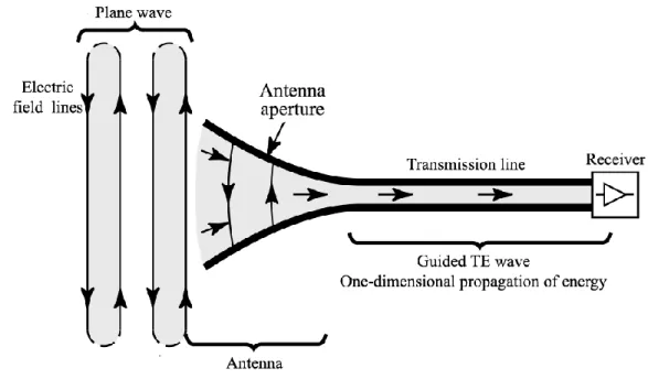
4. ANTENNAS Antenna (aerial) is a media or device for transmitting and receiving radio waves; more precisely, the antenna is the mediator between waveguide and free-space. It efficiently converts the energy of the electromagnetic wave through the transmission line, into the energy that propagates in free-space. Antenna can act as transmitter or receiver, depending on whether it sends or receives data. The transmitting antenna (Figure 19) converts the electromagnetic wave from the transmission line into the electromagnetic wave in the free-space. The receiving antenna (Figure 20) converts the electromagnetic wave from the free-space into the wave in the transmission line. The basic function of an antenna is to adjust the wave from the free-space with the wave within the transmission line (and vice versa), but also to direct the radiated energy into certain parts of the space [26 (pp. 1-18), 27].. Figure 19: Transmitting antenna. Figure 19 shows a transmitting antenna, consisting of a transmitter that generates voltage 𝑽𝑨 that creates distribution of alternating current 𝑰𝑨 , a transmission line (in this case, a waveguide). 29.

and the antenna aperture that transmits an electromagnetic field from the waveguide into a free-space → three-dimensional space. At the boundary between the waveguide and the antenna, electromagnetic field lines resemble the plane wave. As the waves approach the antenna aperture, they take shape of the concentric circles. The more they move away from the source and the antenna itself, they are re-shaped into plane waves again [24, 25, 27].. Figure 20: Receiving antenna. In Figure 20, the opposite process takes place, where electromagnetic waves in the free-space, which are transmitted from the transmitting antenna, spread to the receiving antenna through the waveguide and are delivered to the receiver [24, 25, 27].. 4.1 Antenna parameters In order to describe the characteristics and performance of the antenna, it is necessary to describe its parameters. Antenna parameters are defined in free-space, and depend on the position of the antenna according to the Earth and surrounding objects. Some of the standard antenna parameters include radiation pattern (diagram), antenna gain, polarization, directivity, 30.

field regions, antenna efficiency, radiation intensity and power density. Some of the mentioned parameters will be explained in this chapter [6 (pp. 301-307), 26 (pp. 1-79)].. 4.1.1 Radiation pattern. Beamwidth Antenna radiation pattern (Figure 21) represents the mathematical or graphical display of electromagnetic radiation that characterizes the antenna, in function of three-dimensional spatial coordinates. Essentially, the radiation diagram provides the necessary information for the spatial distribution of electromagnetic radiation around the antenna. The radiation pattern is most commonly referred to the distant radiation (far-field) zone where electromagnetic radiation is represented in the form of plane waves. There are two basic types of radiation pattern – a power diagram represents the spatial distribution of normalized radiation power, and a field diagram represents the normalized amplitude of electric or magnetic fields. The radiation diagram is represented in a logarithmic (decibel) or linear scale in values, relative to the maximum radiation [6 (pp. 301-307), 26 (pp. 25-33)]. Antenna radiation diagram has two planes in the Cartesian coordinate system, which are relevant for its presentation: horizontal and vertical plane. The angle in the horizontal plane is the angle of azimuth, and the angle in the vertical plane is the angle of elevation. The actual illustration of the radiation diagram is actually 3D, shown in Figure 31. In most communication applications during transmission, all electromagnetic energy is required to be directed in the chosen direction.. Furthermore, antenna has only one major (main) lobe and a larger number of minor (secondary) lobes. The major lobe is defined as the lobe in the direction of maximum radiation. The minor lobe is defined as the lobe whose direction of radiation is different from the one in which the main lobe is directed. In a properly constructed antenna system, the minor lobe levels are considerably lower than the major lobe level [26] (pp. 25-33).. 31.

Figure 21: Antenna radiation pattern. The radiation pattern (Figure 22) consists of the following parameters:. 1. Direction of maximum radiation [𝑬𝒎𝒂𝒙 , (𝜣𝟎 , 𝝓𝟎 )] – the direction in which the radiated field has the maximum value; major lobe direction.. 2. Angle of directivity (𝜣𝑫 ) – the angle around the direction of the maximum radiation within which the radiated power density does not fall below half of the maximum radiated power; HPBW → 0.707 for linear field value, 0.5 for linear power value and -3 dB for logarithmic power value.. 3. Beamwidth (𝜣𝒏 ) – the angle between the first null points on both sides of the radiation pattern maximum; FNBW.. 4. Suppression factor of minor lobes (𝒔) – the field strength ratio between the direction of maximum radiation and the direction of the “largest” minor lobe. 32.

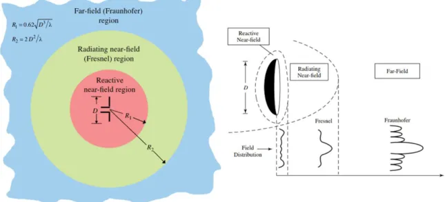
Figure 22: Radiation patterns. Beamwidth is one of the parameters of the radiation pattern. It indicates the angular distance between two identical points, which are on the opposite sides of the radiation pattern maximum. Two types of beamwidths are also mentioned, namely FNBW and HPBW. The relationship between these two beamwidths is given by the expression 𝐻𝑃𝐵𝑊 ≈. 𝐹𝑁𝐵𝑊 2. .. 4.1.2 Field regions The area around antenna consists of three field regions (Figure 23). These are the fields of electromagnetic radiation surrounding the antenna. Given the proximity of the field, the regions 33.

are divided into reactive near-field, radiating near-field (known as the Fresnel region) and a farfield, or Fraunhofer's region. These field regions differ in the intensity of the radiated power, since it is known that the energy decreases with the square of the distance.. Figure 23: Field regions and field distribution. The reactive near-field region surrounds the area around the antenna, where the reactive field prevails. Although the reactive region is near the antenna, a boundary still defines the transition between the regions. The boundary is defined as the distance from the center of the circle that encloses a reactive near-field, and is represented by a mathematical expression. 𝑅1 = 0.62 ∙ √. 𝐷3 𝜆. (4.1). where: 𝑅1 − distance from the center where the antenna is located [m] 𝐷 − largest antenna dimension [m] 𝜆 − wavelength [m]. 34.

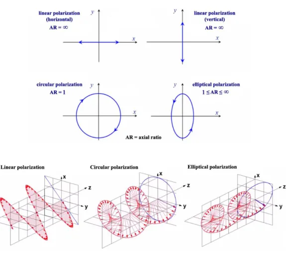
The next area is the radiating near-field, better known as Fresnel’s region. This region is located between reactive and far-field region. In radiating region, the field distribution depends on the distance from the antenna and its dimension. The boundary of the radiation near-field is represented by a mathematical expression. 𝑅2 =. 2 ∙ 𝐷2 𝜆. (4.2). where: 𝑅2 − distance from the center where the antenna is located [m] 𝐷 − largest antenna dimension [m] 𝜆 − wavelength [m]. Both fields have something in common: if the antenna dimension 𝑫 is smaller than its wavelength 𝝀 , the field regions around antenna may not exist.. Lastly, the far-field is located far from the antenna. In this region, the EM field behaves as a plane wave, meaning that changes in the electric and magnetic fields have a uniform distribution in the plane, which is perpendicular to the direction of propagation. If the maximum antenna dimension – 𝑫 is considerably greater than the wavelength 𝝀 , then it can be assumed that the distant zone begins with the distance. 𝟐∙𝑫𝟐 𝝀. from the antenna. This region is called a. Fraunhofer's region [26] (pp. 25-33).. 4.1.3 Polarization From Chapter 4 in Figure 20, the fact that the electromagnetic wave in the far-field acts as a plane wave is taken into consideration. At that distance, the electric and magnetic field vectors are perpendicular to the direction of wave propagation, and they change their direction and. 35.

magnitude in time. The curve described by the top of the electric field vector is defined as polarization (Figure 24). Polarization of EM wave defines the orientation, where maximum power is achieved. Polarization is defined by the following parameters: axial ratio (AR), which is the ratio of large and small ellipse axis, direction in which the electric field vector rotates; clockwise – right and counterclockwise – left, and the direction of large axis, in relation to the reference coordinate system.. Figure 24: Types of polarization. A polarization ellipse shape is defined by ratio between major axis 𝑶𝑨 and minor axis 𝑶𝑩 represents polarization. Knowing these parameters, one can define the axial ratio – 𝑨𝑹, whose values are in the interval between 1 and +∞.. 36.