CHAPTER IV
RESULT AND DISCUSSION
In this chapter, the writer presents the data which had been collected from the research in the field of study. The data were the result of pretest-posttest of experimental group and control group, the result of data analysis, discussion.
A. Result
In this section described the obtained data of the effectiveness of team pair solo technique on speaking performance score of the eighth graders of SMP Negeri 1 Palamgka Raya. The presented data consisted of distribution of pretest score of experiment and control groups and also the distribution of posttest score of experiment and control groups.
1. The Result of Pretest Score of Experimental Group and Control Group
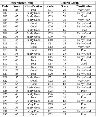
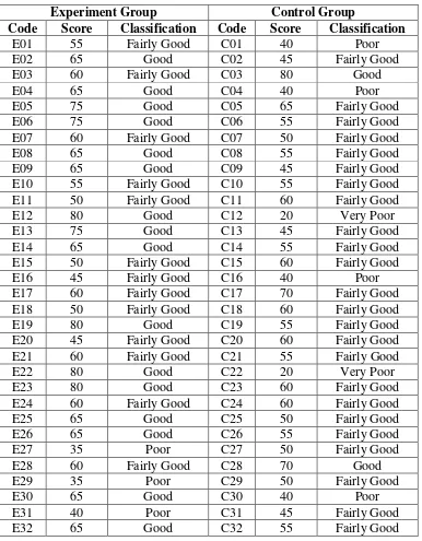
Table 1.6 Pretest Score of the Experiment and Control Group
Experiment Group Control Group
Code Score Classification Code Score Classification
E01 25 Poor C01 20 Very Poor
a. The Result of Pretest Score of Experimental Group
following table in order analyzing the students’ background knowledge of speaking performance score before the treatment. Then, it was presented using distribution frequency in the following table:
Table 1.7 Frequency Distribution of Pretest Experiment Group
Experiment
Frequency Percent Valid Percent Cumulative Percent
Valid
20 2 6,3 6,3 6,3
25 3 9,4 9,4 15,6
35 2 6,3 6,3 21,9
40 3 9,4 9,4 31,3
45 6 18,8 18,8 50,0
50 1 3,1 3,1 53,1
55 6 18,8 18,8 71,9
60 1 3,1 3,1 75,0
65 3 9,4 9,4 84,4
75 2 6,3 6,3 90,6
80 3 9,4 9,4 100,0
Total 32 100,0 100,0
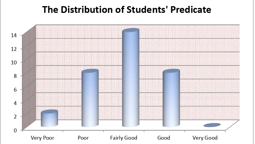
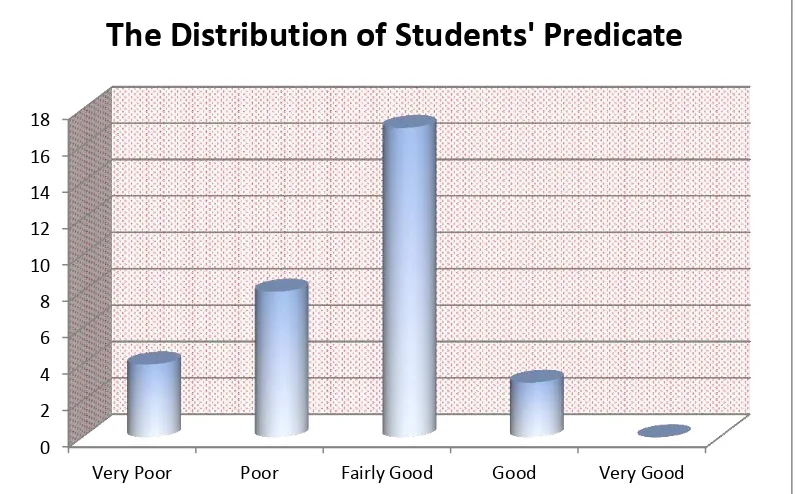
The distribution of students’ predicate in pretest score of experiment group
Figure 1.1 The Distribution of Students’ Predicate in Pretest Score of
Experimental Group
Based on the figure above, it can be seen that the students’ predicate in
pretest score. There were two students who got very poor predicate. They are E-29 and E-31. There were eight students who got poor predicate. They are E-01, E-11, E-15, E-16, E-17, E-18, E-20, and E-27. There were fourteen students who got fairly good predicate. They are E-02, E-03, E-04, E-07, E-08, E-09, E-10, E-14, E-21, E-24, E-25, E-26, E-28, and E-30. There were eight students who got good predicate. They are E-05, E-06, E-12, E-13, E-19, E-22, E-23, and E-32, and there were not students who got very good predicate.
The next step, the writer calculated the scores of mean, median, mode, standard error of mean, and standard deviation using SPSS 21 program as follows.
0 2 4 6 8 10 12 14
Very Poor Poor Fairly Good Good Very Good
Table 1.8 the calculation of Mean, Median, Mode, Standard Error of Mean, experimental group was 80, the lowest score was 20, the result of mean was 50.00, median was 47.50, mode was 45, standard error of mean was 3.086, and the standard deviation was 17.460.
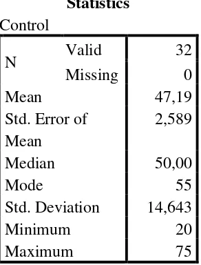
b. The Result of Pretest Score of Control Group
The pretest was conducted on Saturday 21st December 2015 in the VIII 2 class. The students’ pretest score of control group were distributed in the
following table in order analyzing the students’ background knowledge of
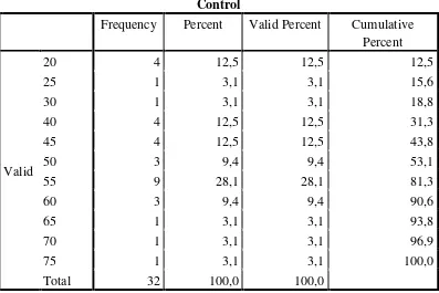
Table 1.9 Frequency Distribution of Pretest Control Group
Control
Frequency Percent Valid Percent Cumulative Percent
Valid
20 4 12,5 12,5 12,5
25 1 3,1 3,1 15,6
30 1 3,1 3,1 18,8
40 4 12,5 12,5 31,3
45 4 12,5 12,5 43,8
50 3 9,4 9,4 53,1
55 9 28,1 28,1 81,3
60 3 9,4 9,4 90,6
65 1 3,1 3,1 93,8
70 1 3,1 3,1 96,9
75 1 3,1 3,1 100,0
Total 32 100,0 100,0
Figure 1.2 The Distribution of Students’ Predicate in Pretest Score of Control
Group
Based on the figure above, it can be seen that the students’ predicate in pretest score. There were four students who got very poor predicate. They are C-01, C-04, C-12, and C-22. There were eight students who got poor predicate. They are C-09, C-13, C-16, C-25, C-27, C-29, C-30, and C-31. There were seventeen students who got fairly good predicate. They are C-02, C-05, C-06, C-08, C-10, C-11, C-14, C-15, C-18, C-19, C-20, C-21, C-23, C-24, C-26, C-28, and C-31. There were three students who got good predicate. They are 03, 07, and C-17, and there were not students who got very good predicate.
The next step, the writer calculated the scores of mean, median, mode, standard error of mean, and standard deviation using SPSS 21 program as follows.
0
Very Poor Poor Fairly Good Good Very Good
Table 2.0 The calculation of Mean, Median, Mode, Standard Error of Mean, and Standard Deviation.
Statistics Control
N Valid 32
Missing 0
Mean 47,19
Std. Error of Mean
2,589
Median 50,00
Mode 55
Std. Deviation 14,643
Minimum 20
Maximum 75
Based on the calculation above, the higher score pretest of control group was 75, the lowest score was 20, the result of mean was 47.19, median was 50.00, mode was 55, standard error of mean was 2.589, and the standard deviation was 14.643.
2. The Result of Posttest Score of Experimental Group and Control Group
Table 2.1 Posttest Score of the Experiment and Control Group
Experiment Group Control Group
Code Score Classification Code Score Classification
a. The Result of Posttest Score of Experimental Group
The posttest was conducted on Saturday 11th January 2016 in the VIII 3 class. The students’ posttest score of experiment group were distributed in the
following table in order analyzing the students’ background knowledge of
speaking performance score before the treatment. Then, it was presented using distribution frequency in the following table:
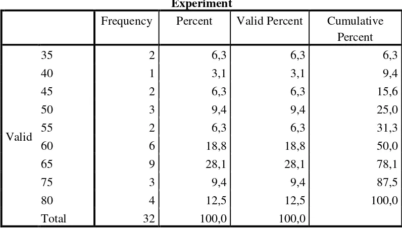
Table 2.2 Frequency Distribution of Posttest Experiment Group
Experiment
Frequency Percent Valid Percent Cumulative Percent
Valid
35 2 6,3 6,3 6,3
40 1 3,1 3,1 9,4
45 2 6,3 6,3 15,6
50 3 9,4 9,4 25,0
55 2 6,3 6,3 31,3
60 6 18,8 18,8 50,0
65 9 28,1 28,1 78,1
75 3 9,4 9,4 87,5
80 4 12,5 12,5 100,0
Total 32 100,0 100,0
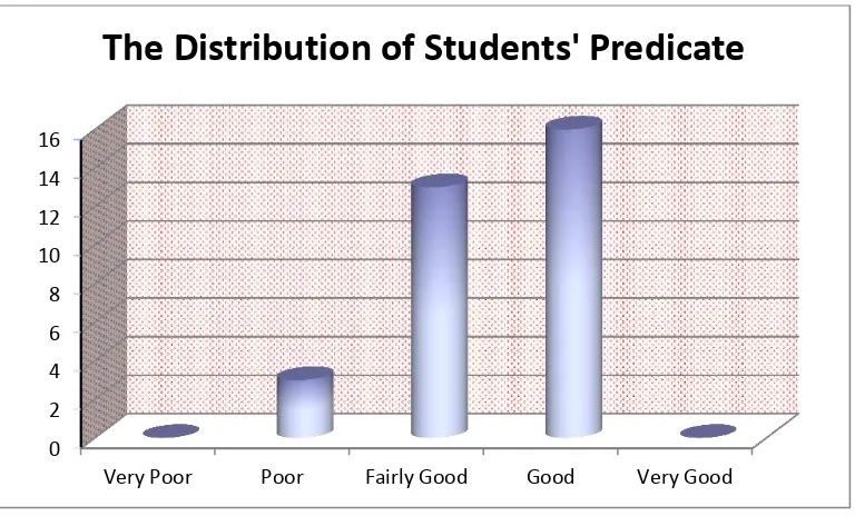
The distribution of students’ predicate in posttest score of experiment group
Figure 1.3 The Distribution of Students’ Predicate in Posttest Score of
Experimental Group
Based on the figure above, it can be seen that the students’ predicate in
posttest score. There were not students who got very poor predicate. There were three students who got poor predicate. They are E-27, E-29, and E-31. There were three teen students who got fairly good predicate. They are 01, 04, 07, E-10, E-11, E-15, E-16, E-17, E-18, E-20, E-21, E-24, and E-28. There were sixteen students who got good predicate. They are 02, 04, 05, 06, 08, 09, E-12, E-13, E-14, E-19, E-22, E-23, E-25, E-26, E-30, and E-32, and there were not students who got very good predicate.
The next step, the writer calculated the scores of mean, median, mode, standard error of mean, and standard deviation using SPSS 21 program as follows.
0 2 4 6 8 10 12 14 16
Very Poor Poor Fairly Good Good Very Good
Table 2.3 The calculation of Mean, Median, Mode, Standard Error of Mean, group was 80, the lowest score was 35, the result of mean was 60.94, median was 62.50, mode was 65, standard error of mean was 2.227, and the standard deviation was 12.600.
b. The Result of Posttest Score of Control Group
The posttest was conducted on Tuesday 5th January 2016 in the VIII 2 class. The students’ posttest score of control group were distributed in the
following table in order analyzing the students’ background knowledge of
Table 2.4 Frequency Distribution of Pretest Control Group
Control
Frequency Percent Valid Percent Cumulative Percent
Valid
20 2 6,3 6,3 6,3
40 4 12,5 12,5 18,8
45 4 12,5 12,5 31,3
50 4 12,5 12,5 43,8
55 8 25,0 25,0 68,8
60 6 18,8 18,8 87,5
65 1 3,1 3,1 90,6
70 2 6,3 6,3 96,9
80 1 3,1 3,1 100,0
Total 32 100,0 100,0
The distribution of students’ predicate in posttest score of experiment group
Figure 1.4 The Distribution of Students’ Predicate in Posttest Score of
Control Group
Based on the figure above, it can be seen that the students’ predicate in
posttest score. There were two students who got very poor predicate. They are 12 and 22. There were four students who got poor predicate. They are 01, C-04, C-16, and C-30. There were twenty three students who got fairly good predicate. They are C-02, C-05, C-06, C-07, C-08, C-09, C-10, C-11, C-13, C-14, C-15, C-17, C-18, C-19, C-20, C-21, C-23, C-24, C-25, C-26, C-27, C-29, C-31, and 32. There were two students who got good predicate. They are 03 and C-28, and there were not students who got very good predicate.
The next step, the writer calculated the scores of mean, median, mode, standard error of mean, and standard deviation using SPSS 21 program as follows.
0 5 10 15 20 25
Very Poor Poor Fairly Good Good Very Good
Table 2.5 The Calculation of Mean, Median, Mode, Standard Error of Mean, and Standard Deviation.
Statistics Control
N Valid 32
Missing 0
Mean 52,03
Std. Error of Mean
2,221
Median 55,00
Mode 55
Std. Deviation 12,563
Minimum 20
Maximum 80
Based on the calculation above, the higher score posttest of control group was 80, the lowest score was 20, the result of mean was 52.03, median was 55.00, mode was 55, standard error of mean was 2.221, and the standard deviation was 12.563.
Table 2.6 The Comparison Result of Pre-test and Post-test of Experimental and Control Group
Experimental Group Control Group
No Code Pretest Posttest Difference Code Pretest Posttest Difference
4. Testing the Normality and Homogeneity a. Normality Test
The writer used SPSS 21 to measure the normality of the data.
Table 2.7 Testing Normality of Posttest Experimental and
Control Group
Kolmogorov-Smirnov Z ,893 ,882
Asymp. Sig. (2-tailed) ,403 ,418
a. Test distribution is Normal. b. Calculated from data.
The table showed the result of test normality calculation using SPSS 21.0 program. To know the normality of data, the formula could be seen as follows:
If Significance > 0.05 = data is normal distribution
If Significance < 0.05 = data is not normal distribution.
higher than the level significance (0.05). Thus, it be concluded that the data was normal distribution.
b. Homogeneity Test
Table 2.8 Testing Homogeneity of Posttest Experimental and Control Group
Test of Homogeneity of Variances Levene
Statistic
df1 df2 Sig.
2,406 6 23 ,060
The table showed the result of homogeneity test calculation using SPSS 21.0 program. To know the homogeneity of data, the formula could be seen as follows:
If Sig. > 0.05 = data is normal distribution
If Sig. < 0.05 = data is not normal distribution
5. Result Data Analysis
a. Testing Hypothesis Using Manual Calculation
To test the hypothesis of the study, the writer used t-test statistical calculation. Firstly, the writer calculated the standard deviation and the error of X1 and X2 at the previous data presentation. It could be seen on
this following table:
Table 2.9 The Standard Deviation and Standard Error of X1 and X2
Variable Standard Deviation Standard Error
X1 12.600 2.227
X2 12.563 2.221
X1 = Experimental Group
X2 = Control Group
The table showed the result of the standard deviation calculation of X1
was 12.600 and the result of the standard error of was 2.227. The result of the standard deviation of X2 was 12.563 and the result of the standard error
was 2.221.
Standard error of mean of score difference between Variable I and Variable II
SEM1– SEM2 = SEM12 + SEM22
SEM1– SEM2 = √
SEM1– SEM2 = √
SEM1– SEM2 = √
SEM1– SEM2 = 3.14521
The calculation above showed the standard error of the differences mean between X1 and X2 was 3.14521. Then, it was interested to the t test
formula to get the value of t test as follows:
t
o=
t
o=
t
o=
t
o=
2.831Which the criteria:
If t-test t-table, Ha is rejected and Ho is accepted
Then, the writer interpreted the result of t-test; previously, the writer accounted the degree of freedom (df) with the formula:
Df = (N1 + N2) – 2
= 32 + 32 – 2 = 62
The writer chose the significant levels at 5%, it means the significant level of refusal of null hypothesis at 5%. The writer decided the significant level at 5% due to hypothesis typed stated on non-directional (two-tailed test). It meant that hypothesis cannot direct the prediction of alternative hypothesis. Alternative hypothesis symbolized by “1”. This symbol could
direct the answer of hypothesis, “1” can be (>) or (<). The answer of
hypothesis could not be predicted whether on more than or less than.
The calculation above showed at the result of t-test calculation as in the table follows:
Table 3.0 The Result of T-Test Using Manual Calculation
Variable T test T table Df
5% 1%
Where:
X1 = Experimental Group
X2 = Control Group
T test = The Calculated Value
T table = The Distribution of t Value
Df = Degree of Freedom
Based on the result of hypothesis test calculation, it was found that the value of t observed was greater than the value of t table at 1% and 5%
significance level or 1.999 <2.831> 2.657 it means Ha was accepted and
Ho was rejected. It could be interpreted based on the result of calculation
that Ha stating that Team Pair Solo was effective technique on speaking
performance of the eight graders of SMP N 1 Palangka Raya was accepted and Ho stating that Team Pair Solo was effective technique on speaking
b. Testing Hypothesis Using SPSS 21.0 Program
The writer also applied SPSS 21.0 program to calculate t-test in testing hypothesis of the study. The result of the t-test using SPSS 21.0 program could be seen as follows:
Table 3.1 Mean, Standard Deviation and Standard Error of Experiment Group and Control Group using SPSS 21.0 Program
Group Statistics
Group N Mean Std.
Deviation
Std. Error Mean Score Experiment 32 60,94 12,600 2,227
Control 32 52,03 12,563 2,221
Table 3.2 The Calculation of T-Test Using SPSS 21.0
t-test for Equality of Means
F Sig. t df Sig.
The table showed the result t-test calculation using SPSS 21.0 program. To know the variances score of data, the formula could be seen as follows:
If Sig. > 0.05 = Equal variances assumed
If Sig. < 0.05 = Equal variances assumed
Based on data above, significant data is 0.840. The result is 0.840 > 0.05 it meant the t-test calculation uses at the equal variances assumed. It found that the result of tobserved is 2.831, the result of mean difference between experiment
B. Discussion
The result of analysis showed that there was significant effect of Team Pair Solo (TPS) technique on speaking performance score of the eighth graders of SMP N 1 Palangka Raya. It can be seen from the means score between pretest and posttest. The mean score of posttest reached higher score than the mean score of pretest (X= 60.94 > 52.03). It indicated that the students score increased after conducting treatment.
In addition, after the data was calculated using t test formula using SPSS 21.0 program showed that the t observed was higher than ttable at 5% and 1%
significance level or 1.999 < 2.831> 2.657. It meant Ha is accepted and Ho is rejected. This finding indicated that alternative hypothesis (Ha) stating that there is significant effect of team pair solo (tps) technique on speaking performance score of the eighth graders of SMP Negeri 1 Palangka Raya was accepted. And the null hypothesis (Ho) that stating that there is no significant effect of team pair solo (tps) technique on speaking performance score of the eighth graders of SMP Negeri 1 Palangka Raya was rejected. Team pair solo technique was effective and supported the previous research done by Chandra Argi Pratiwi and Rosita Amalia that also stated teaching speaking by using team pair solo technique was effective.
problems which initially re beyond their ability. This strategy builds confidence when attempting more difficult content material.
In conducting this research, the writer got some problems. Such us: some students did not participate and wasting time. To overcome those problems above the writer did several ways. First, the writer did controlling intensively to each group. (See p. 22). Teacher divides the students into teams. Each team consists of 4 students. Students work as a team to solve a problem or accomplish a task. In this phase, the teacher should be controlled the students during discussing. Meant, the writer paid attention on the students’ activity in
the group, and warned them if they did not participate. Dealing with the second problem the writer did the class setting. Meant, the class was design to shorten time such as the chairs was arranged based on group.
Those are the result of pretest compared with posttest for experimental group and control group of students at SMP Negeri 1 Palangka Raya. Based on the theories and the writer’s result, Team Pair Solo (TPS) technique gave