A Multifactor Model of Credit Spreads

Submission Cover

21

st

Australasian Finance and Banking Conference

1. Title

A Multifactor Model of Credit Spreads

2. Primary Author

Ramaprasad Bhar

3. Co-Authors (separate with comma)

Nedim Handzic

4. Prizes

Select the prizes for which you would like to be considered (you may pick

more than one).

(For more information about prizes please see the conference web site:

www.banking.unsw.edu.au/afbc

)

Prize Yes/No

Barclay's Global Investors Australia Prize

Yes

BankScope Prize

Sirca Research Prize

Australian Securities Exchange Prize

5. Journals

Select the journals for which you would like to be considered (you may pick

more than one).

Journal Yes/No

Journal of Banking and Finance

Yes

Journal of Financial Stability

6. Conference Proceedings

Yes/No

Would you like your paper (if accepted) to be published by World

Scientific Publishing Co Ltd as a review volume compiling

selected papers?

A Multifactor Model of Credit Spreads

Ramaprasad Bhar

School of Banking and Finance

University of New South Wales

∗

Tel: +61 2 9385 4930

Email:

r.bhar@unsw.edu.au

Nedim Handzic

1

School of Banking and Finance

University of New South Wales

& Tudor Investment Corporation

Tel: +61 405 507 610

Email:

nhandzic@bigpond.com

This Version: 14 August 2008

ABSTRACT

We represent credit spreads across ratings as a function of common unobservable factors of the

mean-reverting normal (Vasicek) form. Using a state-space approach we estimate the factors, their process

parameters, and the exposure of each observed credit spread series to each factor. We find that most

of the systematic variation across credit spreads is captured by three factors. The factors are closely

related to the implied volatility index (VIX), the long bond rate, and S&P500 returns, supporting the

predictions of structural models of default at an aggregate level. By making no prior assumption about

the determinants of yield spread dynamics, our study provides an original and independent test of

theory. The results also contribute to the current debate about the role of liquidity in corporate yield

spreads. While recent empirical literature shows that the level and time-variation in corporate yield

spreads is driven primarily by a systematic liquidity risk factor, we find that the three most important

drivers of yield spread levels relate to macroeconomic variables. This suggests that liquidity risk is

largely driven by the same factors as default risk.

Keywords: Credit Spreads, Macroeconomic Factors, Kalman Filter, State-space model

JEL Classification: C11; C15; G12

A Multifactor Model of Credit Spreads

ABSTRACT

We represent credit spreads across ratings as a function of common unobservable factors of the

mean-reverting normal (Vasicek) form. Using a state-space approach we estimate the factors, their process

parameters, and the exposure of each observed credit spread series to each factor. We find that most

of the systematic variation across credit spreads is captured by three factors. The factors are closely

related to the implied volatility index (VIX), the long bond rate, and S&P500 returns, supporting the

predictions of structural models of default at an aggregate level. By making no prior assumption about

the determinants of yield spread dynamics, our study provides an original and independent test of

theory. The results also contribute to the current debate about the role of liquidity in corporate yield

spreads. While recent empirical literature shows that the level and time-variation in corporate yield

spreads is driven primarily by a systematic liquidity risk factor, we find that the three most important

drivers of yield spread levels relate to macroeconomic variables. This suggests that liquidity risk is

largely driven by the same factors as default risk.

Keywords: Credit Spreads, Macroeconomic Factors, Kalman Filter, State-space model

I. INTRODUCTION

The theoretical link between credit spreads and market variables is established by structural models of

default. Models such as Merton (1974) and Longstaff and Schwartz (1995) are based on the economic

definition of default as the event where a firm's value falls below the face value of its outstanding

debt. The unobservable value of the firm is assumed to follow Brownian motion under the assumption

of risk-neutrality, allowing the calculation of default probabilities and an endogenous recovery rate.

Credit spreads are attributed entirely to the risk-neutral expected default loss, which is positively

related to firm leverage and volatility in the firm value. An increase in the firm value through positive

equity performance has the effect of reducing leverage and credit spreads. Under the assumption of

risk-neutrality the firm value process has a drift rate equal to the risk-free rate. The models predict

that an increase in treasury yields increases the drift of the firm value process, leading to lower credit

spreads.

In practice, structural models tend to underestimate short-term credit spreads. The use of smooth

processes to represent the firm value may exclude the possibility of default by high grade issuers in

the short term, which is inconsistent with the observed role of surprise in credit markets. In contrast,

reduced-form models are flexible enough to empirically fit the term structure of credit spreads, but

they do not provide an economic interpretation of default. Reduced form models such as Jarrow and

Turnbull (1995) and Duffie and Singleton (1999), define exogenous stochastic processes for the

arrival time of default and exogenous recovery rates. An additional class of models combines the

advantages of both structural and reduced-form approaches by incorporating exogenous effects such

as jump-diffusions (Zhou 1997) in the firm value process to allow for surprise default. An empirical

overview of structural models by Eom, Helwege and Huang (2004) reveals that existing models

cannot simultaneously fit both high-grade and low-grade bond spreads. They conclude that more

accurate models would need to correct the common tendency to overstate the credit spreads of firms

with high leverage or volatility while at the same time understating the spreads of high-grade bonds.

To the extent that credit spreads reflect expectations on future default and recovery, we would expect

aggregate credit spread indices to vary with macroeconomic variables such as interest rates, stock

market returns and market volatility. In general, low-grade bond spreads are observed to be closely

related to equity market factors (Huang and Kong, 2003) while high-grade bonds are more responsive

to treasury yields. Kwan (1996) finds that individual firm yield spread changes are negatively related

to both contemporaneous and lagged equity returns of the same firm. On the other hand, lagged yield

spread changes do not help explain current equity returns. Campbell and Taksler (2003) show credit

increase in market and firm volatility documented by Campbell et al. (2001) is consistent with the

steady rise in credit spreads throughout the 1990s.

Duffee (1998) finds that investment-grade yield spreads vary inversely with treasury yields, with the

effect being strongest for callable bonds. As treasury yields fall, the prices of callable bonds increase

by a lower proportion than treasuries due to the increasing value of embedded calls, leading to wider

credit spreads. Given that the proportion of callable bonds is higher among lower quality issuers

(Chen et al, 2007), call features may add to the interest rate sensitivity of lower-grade bond indices2.

A negative relationship between investment-grade spreads and treasury yields is also estimated by

Longstaff and Schwartz (1995) while Collin-Dufresne et al (2001) show that credit spreads have

increasingly negative sensitivities to interest rates as ratings decline across both investment and non

investment grade bonds. In a study of only high-yield bonds, Fridson and Jonsson (1995) find no

significant relationship between credit spreads and treasury rates, which is more consistent with the

idea that low-grade bonds are far more responsive to equity variables than interest rate variables.

While there is strong empirical evidence of a negative relationship between investment-grade spreads

and treasury yields, there is no consensus on its economic causes. Intuitively, lower yields should lead

to narrower yield spreads through lower borrowing costs that increase the probability of survival.

However, falling treasury yields, particularly in the shorter maturities, also tend to be a feature of

recessionary periods when default risk rises and central banks typically lower short-term rates. One

recent example of this is the sub-prime crisis, beginning in August 2007, during which short-term

treasury yields declined to historical lows while credit spreads widened to historical highs. Duffee

(1998) concludes that despite the links of both treasury yields and corporate bond spreads to future

variations in aggregate output, it is not obvious that these links explain their observed negative

relationship, or that yield spreads are determined by credit quality. To link credit spreads to interest

rates and expected aggregate output, the empirical literature has also focused on the slope of the

treasury curve, defined as the spread between long-term and short-term yields and often used as a

barometer of future economic conditions. Estrella and Hardouvelis (1991) associate a positive slope

of the yield curve with future increases in real economic activity, hence an increase (decrease) in the

slope of the yield curve should indicate a lower (higher) probability of a recession, in turn reflected in

lower (higher) credit spreads. This idea is supported by the findings of Papageorgiou and Skinner

(2006) that investment-grade credit spreads are negatively related to changes in both the level and the

slope of the treasury curve. In addition they estimate that the negative relationship between credit

spreads and the treasury slope is relatively stable over time.

The empirical literature to date supports both the significance and the direction in which structural

model variables influence credit spreads, however, recent studies demonstrate that these variables

2

alone are not sufficient to fully explain either the levels or changes in credit spreads. Collin-Dufresne

et al. (2001) regress credit spread changes of individual bonds on the changes in treasury yields, the

slope of the yield curve, equity index returns, and index volatility, estimating that these variables

explain only about 25% of the variation in credit spreads. In addition, the slope of the yield curve is

not a significant determinant of credit spread changes when the other variables are taken into account.

Using principal components analysis on the residuals they find that the changes in residuals across

individual bonds are dominated by a single common systematic component that has no obvious

relationship to variables from the interest rate and equity markets. Their conclusion is that yield

spread changes are only partly accounted for by the economic determinants of default risk.

To estimate how much of the yield spread levels can be accounted for by default risk, Huang and

Huang (2003) calibrate a diverse set of structural models to actual historical default losses then use

them to generate theoretical values of credit spreads. In each case the model-based spreads are well

below the average observed spreads, suggesting that default risk accounts for only a small fraction of

yield spreads. The proportion explained by default risk is highest for low-rated bonds, and decreases

for higher-rated bonds that have low historical default losses. The inability of theoretical risk variables

to account for most of the levels or changes in yield spreads is sometimes referred to as the ‘credit

spread puzzle’. Similar to the problem of the equity premium puzzle, the expected returns on

corporate bonds, like equities, seem well above those justified by the risks. The explanation of the

credit spread premium puzzle has focused on both the presence of additional risks as well as

associated risk premiums. Elton, Gruber, et al. (2001) estimate that expected loss accounts for less

than 25% of the observed corporate bond spreads, with the remainder due to state taxes and factors

commonly associated with the equity premium. Similarly, Delianedis and Geske (2002) attribute

credit spreads to taxes, jumps, liquidity and market risk. Factors associated with the equity premium

include the Fama and French (1996) ‘High-minus-Low’ (HML) factor, found by Huang and Kong

(2003) to account for a significant component of low-grade credit spread changes. The significance of

Fama-French factors is also supported by Joutz et al (2001), who conclude that credit spreads are

determined by both default risk and systematic market risk.

Structural models contain the assumption that default risk is diversifiable, since yield spreads are

assumed to reflect only default loss, with no risk premium for either default risk or the risk of

market-wide changes in spreads. Jarrow et al (2001) show that jumps-to-default in credit spreads cannot be

priced if defaults across firms are conditionally independent and if there is an infinite number of firms

available for diversification. One explanation for the credit spread puzzle is the potential for firms to

default on a wide scale not seen historically, a risk that is difficult to eliminate by diversification and

is therefore priced by investors. It is also observed that defaults across firms tend to be correlated and

incorporate a strongly cyclical market price of risk that increases along with default losses during

recessions. Another explanation for wide credit spreads is that idiosyncratic risk is priced as well as

systematic risk. Amato and Remolona (2003) argue that due to the highly skewed returns in corporate

bonds, full diversification requires larger portfolios than typically needed for equities. Given the

limited supply of bonds, high transaction costs, and possible constraints on portfolio expected losses,

full diversification is difficult to achieve, and it is possible that in practice portfolio managers require

a risk premium associated with individual bond value-at-risk. Recent studies confirm the presence of

both a firm-specific default risk premium as well as a market risk premium. Drisesen (2005)

distinguishes between the market-wide changes in credit spreads and individual credit spread

jumps-to-default, finding that both components are priced. Similar results are obtained by Gemmill and

Keswani (2008), who show that most of the credit spread puzzle can be accounted for by the sum of a

systematic risk premium and a larger idiosyncratic risk premium. While supporting these conclusions,

Collin-Dufresne et al (2003) also suggest that it is not surprise default itself that attracts a significant

premium, but rather it is the potential for credit events of large individual firms to trigger a flight to

quality in the treasury market and cause market-wide increases in credit spreads. So even without

directly violating the assumption of conditional independence of defaults across firms, idiosyncratic

default risk could matter due to its potential to impact market-wide liquidity, which highlights the

difficulty of separating the role of default and liquidity in driving credit spread levels.

A recent stream of literature focuses on the role of liquidity in explaining both the levels and

time-variation of credit spreads. The idea that liquidity is an important and priced determinant of yield

spreads is not new, with Fisher’s (1959) hypothesis being that the risk premium of individual bonds

consists of two main components: a default component and a ‘marketability’ component. The default

component is in part a function of a firm’s earnings variability and debt ratio, measures that directly

correspond to the leverage and asset volatility variables in structural models, while the marketability

component is a function of the outstanding issue size. There is no universal proxy for liquidity risk,

but measures used in previous studies include the bid-ask spread, trade frequency, the proportion of

zeros in the time-series of a bond’s returns, a bond’s age, amount outstanding and term to maturity.

Perraudin and Taylor (2003) estimate that liquidity premiums are at least as large as market risk

premiums and far larger than expected default losses. De Jong and Driessen (2006) estimate the

liquidity risk premium on US corporate bonds at 0.6% for long-maturity investment-grade bonds and

1.5% for speculative-grade bonds. Recent studies estimate the non-default component of credit

spreads directly by subtracting credit default swap (CDS) premiums from corresponding corporate

bond yield spreads. Being simply contracts, CDS are regarded as more pure reflections of credit risk3.

This idea is supported by the findings of Ericsson et al (2005) that CDS premiums are driven by the

3

theoretical determinants of credit risk (the risk free rate, leverage and volatility), but that in contrast to

the results of Collin-Dufresne et al (2001) on corporate bond yield spreads, there is only weak

evidence of a common residual factor affecting CDS premiums. The CDS-based non-default

component estimated by Longstaff et al (2005) is strongly time-varying and related to both

bond-specific and market-wide measures of illiquidity. There is a strong cross-sectional relationship

between the non-default component and individual measures of liquidity such as the bid-ask spread

and issue size. The time-series variation of the non-default component is related to macroeconomic or

systematic measures of liquidity risk such as i) the spread between on-the-run and off-the-run treasury

yields, ii) flows into money market funds, and iii) level of new issuance into the corporate bond

market. The cross-sectional results of Longstaff et al (2005) are consistent with equity market

evidence of Amihud and Mendelson (1986) that market-average returns are an increasing function of

bid-ask spreads, while the time-series results are consistent with the presence of a single common

systematic factor found by Collin-Dufresne et al (2001), as well as evidence of systematic liquidity

risks in interest rate markets in Duffie and Singleton (1997), Liu et al (2004) and Longstaff (2004).

Liquidity risk itself has also been found to be a positive function of the volatility of a firm’s assets and

its leverage, the same variables that are seen as determinants of credit risk (Ericsson and Renault,

2006).

Our aim is to estimate the factors driving the dynamics of yield spread levels directly from the data,

without prior assumption about the specific economic variables that yield spreads could be related to.

Based on existing evidence, we take the view that the time-variation in credit spreads is driven by two

classes of factors that are non-stationary and mean-reverting, respectively. Our initial guess is that the

first group of factors is likely to relate to default risk and have low rates of mean-reversion that reflect

relatively persistent macroeconomic conditions. The second group could relate to liquidity premiums

that are presumed to change with noisy short-term supply and demand shocks. Given that credit risk

explains a lower proportion of high-grade spreads than low-grade spreads, we would then expect

high-grade spreads to have stronger mean-reversion that reflects changes in liquidity due to

supply/demand. However, from Figure 1 it appears that non investment-grade spreads have far more

noise than investment-grade spreads, suggesting that the default risk component may be more highly

mean-reverting than the remaining component. One indication this may be true for corporate yield

spreads is the study of swap spreads by Liu et al (2006), finding time-varying components relating to

both liquidity and default risk, but where the default component is highly mean-reverting and with a

flat term structure, while the liquidity component is more persistent and with a steep upward-sloping

term structure. It is worth noting that spikes in the lowest-grade spread indices resemble the behavior

of the VIX index over the same period. These could be interpreted as short-term increases in default

variations, we observe that while the two bond classes behave in fundamentally different ways during

particular sub-periods, they also appear to have different exposures to shared common short-term

shocks throughout the sample period.

This study assumes that the time-variation in credit spreads across ratings classes is driven by a

common set of unobservable factors to which each observed spread is exposed with some unknown

sensitivity. We aim to answer the following questions: 1) how many factors are required to explain the

evolution of ratings-based spread indices, 2) what are the exposures of individual indices to each

factor, and 3) what economic variables, if any, could be proxies for the factors.

Our choice of the state-space methodology is motivated by its advantage of allowing for both

time-series and cross-sectional data simultaneously. It also provides a new and opposite approach to the

existing literature on credit spread determinants. Most empirical studies on credit spreads adopt a

general-to-specific approach where a range of known potential determinants is tested for statistical

significance using OLS regressions. In contrast, state-space models require only an assumption about

the structure of the factors that can then be estimated directly from the observed data. Another

advantage of state-space models is that they can be applied to both stationary and non-stationary

variables. OLS estimation on the other hand requires that both dependent and independent variables

are stationary, forcing most studies to focus on explaining the changes in credit spreads as a function

of changes in independent variables. In this study we analyze the dynamics of credit spread levels

directly.

Given an assumed parametric process form for the latent factors, the Kalman Filter maximum

likelihood method can be applied to simultaneously estimate 1) the parameters of each factor process,

2) the sensitivities or loadings of each observed series to the individual factors, 3) the realizations of

the factor series, and 4) the covariance matrix of the model errors. The Vasicek (1977) normal

mean-reverting process is chosen for the factors since, depending on the size of its mean-reversion

coefficient, it is suitable for representing both non-stationary (presumed macroeconomic) as well as

stationary (presumed microeconomic) determinants of credit spreads. A multi-factor Vasicek form is

also supported by the findings of Pedrossa and Roll (1998) that Gaussian mixtures can capture the

fat-tailed distributions of credit spreads.

Early applications of the state-space model in finance literature have focused on the term structure of

treasury rates. Babbs and Nowman (1999) find that a three-factor Vasicek model adequately captures

variations in the shape of the treasury yield curve, with two factors providing most of the explanatory

power. Chen and Scott (1993) and Geyer and Pichler (1999) reach similar conclusions based on a

multifactor CIR (1985) model, and find the factors to be closely related to the short rate and the slope

allow for additional factors to explain swap or corporate bond yields. Liu, Longstaff, and Mandell

(2006) separate the liquidity and credit risk components of swap spreads through a five-factor model

of swap yields. Swap yields consist of three factors driving treasury yields, one influencing credit risk,

and the remaining one influencing liquidity risk. Similarly, Feldhutter and Lando (2008) decompose

the factors driving the term structure of the swap yield spreads into three factors driving the risk-free

rate, two affecting credit risk and one relating to the liquidity premium or ‘convenience yield’

contained in treasury yields over the risk-free rates. They find that while credit risk is important, the

strongest determinant of swap spreads is the convenience yield contained in treasury prices. Jacobs

and Li (2008) use the state-space approach to estimate a reduced-form model of default, where the

probability of default is modeled directly as a stochastic volatility process. They find that the addition

of a second, volatility factor to the level factor in the diffusion of default probabilities leads to

significant improvements in both in-sample and out-of-sample fits for credit spreads.

Our work is a natural progression in the application of state-space methodology from treasury yield

levels to corporate yield spreads. We apply the state space methodology directly to credit spreads to

find both the number of factors and compare their behavior to well-known macroeconomic variables.

This is the first work to relate the estimated factors driving corporate yield spreads to variables from

II. DATA

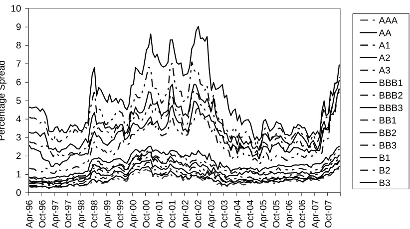
All data is from Bloomberg with observations taken at the end of each month Apr-96 to Mar-08. We

use the 10-year maturity industrial corporate bond yield indices of 14 available ratings: AAA, AA,

A1, A2, A3, BBB1, BBB2, BBB3, BB1, BB2, BB3, B1, B2, and B3. Bloomberg ratings are

composites of S&P and Moody’s ratings, with bonds rated BB1 or lower considered sub-investment

grade. The yield indices are converted into credit spreads by subtracting the 10-year benchmark bond

yield from each. Other variables sourced are the option-implied volatility index of the S&P500 (VIX)

and the S&P500 level.

III. METHOD

A. The Multifactor Vasicek Model in State Space Form

For a given term to maturity, each of n observed credit spread indices by rating

is expressed as a function of m independent latent factors or states

}

X

of the Vasicek form. Changes in the j-th observed series are a linear

combination of the changes in m latent factors weighted by factor loadings

a

. Each

factor evolves according to its three parameters: the long-term mean

jt

θ

, the speed of mean-reversion

κ

4

, and the volatility

σ

. In continuous time,

∑

₌

The application of the Kalman Filter algorithm to estimate the factor loadings, the process parameters

}

and the realization of the state vector over time

, requires that the model is expressed in state space form. State space

representation consists of the measurement equation and the transition (or state) equation.

m

t

The measurement equation (3) maps the vector of observed credit spreads to the state

vector via a ‘measurement matrix’

)

and errors in the sampling of observed series are allowed through n jointly normal error terms

ε

(nx

1

)

that have zero conditional means and covariance matrix

H

(

n

×

n

)

. Since the computational burden of estimating a full error covariance matrix H increases rapidly with additional observed series, most

studies assume error independence. In state-space models of the treasury curve, (Chen and Scott

(1993), Geyer and Pichler (1996), and Babbs and Nowman (1999)) a diagonal matrix with elements

was used to capture the effects of differences in bid-ask spreads across n maturities. In

this study we choose the same form to allow for different bid-ask spreads across n bond quality

groups. The state equation (4) represents the discrete-time conditional distribution of the states. The

terms of the equation follow directly from the discrete form of the Vasicek model for interval size

:

Innovations in the states occur through the normal ‘noise’ vector

η

t, with covariance matrix Q. It is

assumed that the sources of noise in the state and measurement equations are independent.

In state-space representations of affine models of the term structure, where the observed series

correspond to specific maturities, the elements of the measurement matrix Z and the intercept vector

D are usually closed-form functions of the term to maturity, the parameters of each risk factor, factor

correlations, and the market risk premium associated with each factor. The difference in this study is

that the observed series represent different ratings for a single maturity, without a prescribed formula

linking the observed series via factor process parameters. Instead, we estimate the measurement

matrix directly by maximum likelihood, along with the process parameters. To reduce the number of

Based on numerous experiments we find no observable impact of this assumption on either the

estimated factor realizations or the sensitivities of the observed series.

B. The Kalman Filter

At each time step t, the filtered estimate of the realized state vector consists of a predictive

component , based on information to up to and including time t – 1 , and an updating component

incorporating observations at time t. The predictive component of is the conditional mean of ,

, which is the optimal estimator of . For

The estimate is defined as the sum of and an error-correction term weighted by the

Kalman Gain matrix . The higher the terms of the Kalman Gain the more responsive is to

new data.

The recursive equations are started with guesses for the initial state vector and covariance matrix

. In practice, to ensure that the state vector adapts quickly to the first few observations, the initial

state noise covariance should be set to an arbitrarily high number so that the Kalman Gain is close

to a vector of ones. With further observations it is expected that the covariance terms and the Kalman

gain will decrease and stabilize, resulting in a more constant mix of the predictive and error-correcting

term in generating state vector estimates. The number of time-steps required for the Kalman Gain to

stabilize is usually referred to as the 'burn-in' phase. The part of the estimated state vector coinciding

with the burn-in phase is typically excluded in further analysis.

C. Fitting the Model

The state parameters

ψ

, the elements of the measurement matrix

Z

, and the measurement error covariance matrix

H

are estimated by maximizing the log-likelihood function (13) that follows directly from the prediction error decomposition. Given guesses for

ψ

,

Z

, and

H

, and fixed

initialization values

X

₀, and

Σ

₀, the log-likelihood is

In maximizing the log-likelihood function we force all the factor loadings of the first observed credit

spread series (AAA) to equal 1, so that the first observed series is a non-weighted sum of the latent

factors. We add this assumption as a way of ensuring that loadings and factor realizations are scaled

IV. RESULTS

One, two, and three-factor models are estimated for the period Apr-96 to Mar-03 as well as the full

sample period Apr-96 to Mar-08. We are interested in how model estimates are impacted by the

changing economic environment. From Apr-96 to Mar-03 lower-grade credit spreads generally

increased until reaching their peak in Mar-03 (Figure 1). In the period that followed credit spreads

generally narrowed and remained low until 2007. The full sample period includes three major shocks

to liquidity: the LTCM crisis of 1998, the bursting of the technology bubble and increase in corporate

default rates in 2002, and the sub-prime mortgage crisis starting in 2007.

A. Results for Apr-96 to Mar-03

Table 1 shows the estimates for the mean-reversion speed (

κ

), mean (µ), and volatility (

σ

) of each Vasicek factor. The log-likelihood, AIC, and BIC criteria are highest for the three-factor model, under

which all parameters (with the exception of one mean) are highly significant. The marginal

improvement in the log-likelihood from the addition of a third factor is far smaller than for a second

factor, suggesting that a 3-factor model is sufficient in capturing the common sources of variation in

credit spreads. For comparison, the log-likelihoods for the one, two, three, and four-factor models are

1246.0, 1840.6, 2040.6, and 2100.10, respectively. The parameter estimates for factor 4 in a

four-factor model are largely insignificant5, supporting the choice of the three-factor model.

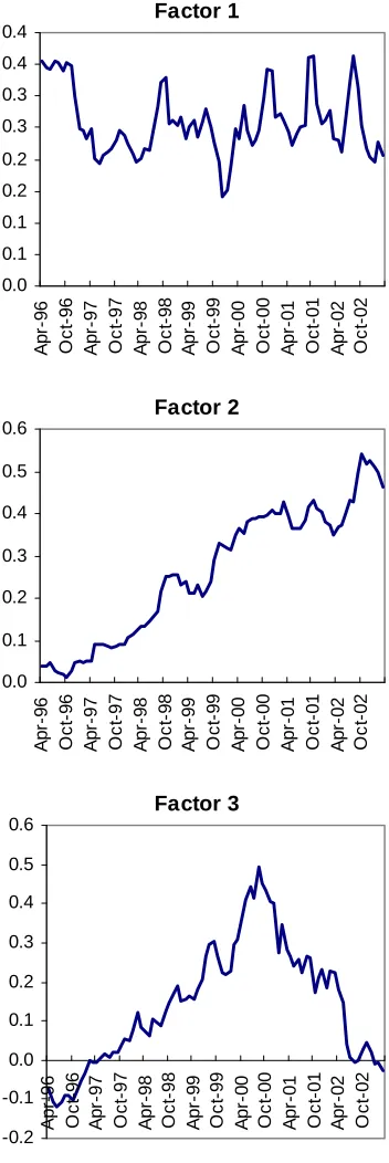
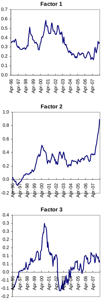
The extracted factor under the one-factor model (Figure 2.1) resembles a weighted average of the 14

observed series. Allowing for a second factor (Figure 2.2) reveals two distinct smooth processes as the

drivers of the cross-section of credit spreads, while in the three-factor model an additional more noisy

process is identified (Figure 2.3). In the three-factor model the half-life is 2.8 months for factor one,

4.1 years for factor two, and 1.6 years for factor three. The factors under the three-factor model are

compared to well-known economic time-series in Figure 3. Under the three-factor model, the noisy

first factor resembles the VIX for most of the sample period, the second resembles the (negative of)

10-year bond rate, and the third the S&P500 level6. The correlations are 0.08 between factor 1 and the

VIX, -0.74 between factor 2 and the long bond rate, and 0.92 between factor 3 and the S&P500 level.

If a “burn-in" phase of the first 12 months is excluded under the Kalman Filter approach, the

correlation between factor 1 and the VIX increases from 0.08 to 0.47. Given the results of Campbell

and Taksler (2003) linking credit spreads to the average of individual firm volatilities, it is possible

5

A parameter is significant at the 5% level if the estimated parameter divided by its standard error is greater than 1.96 in absolute value. The standard errors of the estimated parameters are calculated using a finite-difference estimate of the Hessian matrix, as outlined in Hamilton (1994).

6

that factor 1 is more closely related to measures of the average of individual firm implied volatilities

than it is to the VIX which measures the volatility of the market average returns.

The estimated loadings of the observed series to each factor in the three-factor model are shown in

Table 2 and Figure 2.3. Are the sensitivities to the factors consistent with theory? The shape of the

loadings on the first factor suggests that equity volatility risk has a positive impact on all credit

spreads and that exposure to it increases with declining credit quality. To the extent that equity

volatility is a proxy for a firm's asset value volatility, this result is consistent with the prediction of

Merton (1974) that the probability of default and credit spreads increase with higher asset value

volatility. The sharpest increase occurs in the crossing from investment to sub-investment grade

bonds, which is consistent with the observations of Huang and Kong (2003) and others that

lower-grade bonds are more sensitive to equity market variables than high-lower-grade bonds.

The positive loadings on factor two and its negative correlation with the level of the 10-year treasury

yield are consistent with the strong empirical that increases in treasury yields lower credit spreads.

The loadings are also consistent with the finding of Colin-Dufresne et al (2001) that the sensitivity of

credit spread changes to interest rates increases monotonically across declining rating groups.

The sensitivities to factor 3, which is closely correlated to the S&P500, change sign from positive to

negative as bonds move from investment to sub-investment grade. The estimated positive relationship

between equity market performance and investment grade spread indices is at odds with the Merton

(1974) model since according to the model, higher equity values increase the value of a firm's assets

relative to its fixed level of debt, lowering its probability of default. A possible explanation is that the

positive equity performance throughout the 1990s coincided with rising aggregate debt levels during

the same period, with highest rated firms raising their leverage the most. The negative effect of higher

asset values on spreads may have been more than offset by the positive effect of higher leverage in the

case of higher-grade firms. Changing investor risk preferences may also have played a role. It is

possible that for all but the lowest credits, prolonged positive equity market performance contributed

more to the substitution out of corporate bonds, in favor of equities, than to higher bond values

through improved creditworthiness.

B. Results for Apr-96 to Mar-08

We repeat the analysis for the full sample period and report the results in tables 3 and 4 and figures 5

to 7. The signs of the correlation coefficients between the factors and macroeconomic variables in the

three-factor model remain the same as for the first period: factor 1 and the VIX at 0.71; factor 2 and

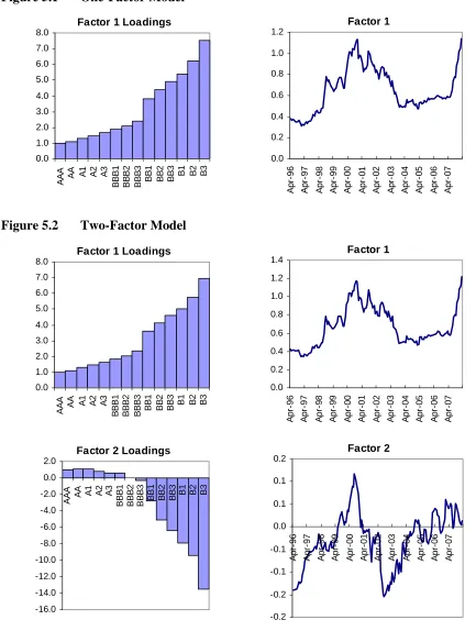
the long bond rate at -0.54; factor 3 and the S&P500 at 0.76. The general shapes of the loadings and

their signs remain unchanged for the 3-factor model, with the exception that loadings on factor 3 are

more strongly negative for non-investment grade debt for the full period. This reflects changing

Mar-03. The lack of a strong direction in the relationship between low-grade spreads and the equity

market is reflected in the estimated loadings of low-grade spreads on factor 3 being close to zero for

the first period. For most of the period that followed (Apr-03 to Mar-08) non-investment grade

spreads steadily declined, with lowest grade spreads declining the most, while at the same time the

S&P500 trended upwards. This feature most likely contributes to the estimated loadings of low-grade

spreads being more negative and varied across ratings when based on the full sample period. There is

also a change in the shape of the loadings on factor 2 for the full period. The loadings peak for the

highest-rated non investment grade index (BB1) but then slowly decline with worse ratings. This is in

contrast to the finding of Collin-Dufresne et al (2001), supported by our estimates for Apr-96 to

Mar-03, that interest rate sensitivities increase monotonically with declining ratings. We note that for the

full period factor 2 is less closely correlated to the long bond yield (coefficient of -0.54), than for

Apr-96 to Mar-03 (coefficient is -0.74), and that the factor loadings across the two periods are therefore

not entirely comparable. However, the shape of the loadings for the full period raises the question of

whether for indices of lower quality than those covered in Collin-Dufresne et al (2001) and this study,

the sensitivities to interest rates would decline further across declining ratings. The possibility is also

raised by the findings of Fridson and Jonsson (1995), that there is no significant relationship between

high-yield spreads and treasury levels.

We find none of the extracted factors in models containing between one to four factors to be

correlated to the slope of the treasury curve, either in the spot or forward yields, contemporaneously

or with a lag. This is consistent with the findings of Collin-Dufresne et al (2001) that the treasury

slope does not help explain credit spread changes, but the result remains surprising given that the

treasury curve is commonly used as an indicator of future economic conditions by market participants.

One explanation is that the slope of the treasury curve contains no useful information beyond that

already contained in the combination of equity returns, volatility and interest rate levels. Another is

simply that the period Apr-96 to Mar-08 contains highly contrasting relationships between credit

spreads and the treasury slope, due to the sub-prime crisis. The period since August 2007 has been

marked by rapidly widening credit spreads while at the same time fears of stagflation, high inflation

and low growth, contributed to short-term treasury yields reaching historically low levels relative to

long-term yields. Hence the end of the sample period is marked by a strong positive contemporaneous

relationship between the slope of the treasury curve and general credit spread levels, which is in

contrast to the negative relationship previously documented by Papageorgiou and Skinner (2006).

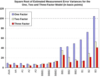
We examine the estimated measurement error variances, defined as the diagonals of matrix H in the

Measurement Equation (3). Figure 8 shows the square-roots of the error variances across rating

classes for the one, two, and three-factor models. As expected, for each model the lowest-rated bonds

variances fall sharply across ratings with the addition of a second factor, particularly for

sub-investment grade bonds. The addition of a third factor does not lead to a large reduction in variances,

which is similar to the modest impact of a third factor on the maximum likelihood. We note that in the

two and three-factor models the measurement error variances also peak around the middle ratings,

which is in contrast to the more monotonic shapes of the loadings on each factor, across ratings. The

variances increase as indices approach the cross-over point between investment and non-investment

grade bonds, with a local maximum for the BB1 index which is the highest-rated non-investment

grade index. Both the shape and magnitude of the error variances are comparable to the results of

Babbs and Nowman (1999), where a multifactor Vasicek model is used to fit the term structure of 8

observed treasury yields across maturities (0.25, 0.5, 1, 2, 3, 5, 7, and 10-year). In that study, the

errors on longer maturities are the highest and decline sharply with the addition of a second factor.

The middle maturities around the two-year series have higher error terms than the surrounding

maturities.

We provide two possible explanations for the pattern in the error variances. Firstly, the time-series of

the first two factors are closely related to averages of the investment-grade bonds and non-investment

grade indices, respectively. We would expect that the further an observed index is from the ‘average’

investment-grade or non-investment grade series, the less precisely it will be captured by the two first

and most important factors. A second explanation is that the observed BB1 index is a relatively noisy

proxy for the yield spreads of BB1 quality. From Figure 1 it can be observed that the BB1 index

closely follows investment-grade bonds early in the sample period, but follows non-investment grade

bonds more closely for the remainder of the period. This changeover could be related to changes in

the composition of the BB1 index, or changes in the pricing of included bonds that does not get

reflected by rating changes. The finite sample of bonds within any rating class creates the potential for

measurement errors in the relative pricing of various rating indices, and it is possible that these are

more pronounced for indices near the cross-over point between investment and non-investment grade.

The fact that the estimated measurement error variances peak around the crossing point of rating

classes while the factor loadings remain relatively smooth can be interpreted as the effectiveness of

state-space models in separating the idiosyncratic and systematic effects. Given a wide enough

cross-section of time-series, the features of individual series that are not common to multiple indices can be

expected to be absorbed into higher measurement error variances, while leaving factor loadings

relatively smooth across the series.

We also analyze the time-series of the fit errors under a three-factor model. Table 5 shows that for

each index the average fit errors are close to zero and strongly stationary based on ADF unit root tests.

We take this as support for the multifactor Vasicek as an unbiased model of credit spreads across

The results for both periods suggest that all credit spreads vary in response to three common

systematic factors that have proxies in the VIX, the long bond rate, and S&P500 returns. The

co-movement between the factors and the variables is particularly evident from the beginning of the

sub-prime crisis. Figure 6 shows that from the second half of 2007 factor 1 sharply increased as well as

the VIX, factor 2 increased with (the negative of) the long-bond rate, and factor 3 declined with the

S&P500 level.

However, the ability of the three factors to explain observed spreads can rapidly decline during

financial crises, as shown by the conditional density likelihoods in Figures 4 and 7. Log-likelihoods

dropped during the LTCM liquidity crisis of August 1998, the end of the technology bubble in 2002,

and since the start of the 2007 sub-prime mortgage crisis. The implication is that credit spreads

reached levels that were not accounted for or fully reflected by the macroeconomic conditions at those

times. Interestingly, during the LTCM crisis a two or three-factor model does not improve the fit over

a one-factor model. One interpretation is that this crisis was of a more exogenous nature and more

specifically relating to changes in credit market liquidity than changes in the macroeconomic outlook.

While the end of the bubble in 2002 and the sub-prime crisis both had long-lasting impacts real

economy, reflected in lower yields, lower equity returns and higher volatility, the LTCM crisis was

characterized by a relatively sharper increase in volatility and smaller changes in rate and equity

returns. It is likely that almost all of the change in credit spread levels during LTCM is explained by

the sharp rise in factor 1 which is representative of the VIX, which is in turn closely related to

liquidity risk. The sharp falls in log-likelihood that accompany the largest market moves point either

to the presence of additional risk factors and risk premiums that are not captured by the Vasicek form,

V. CONCLUSION

This study concludes that most of the systematic variation in credit spread indices by rating is

explained by three factors. The factors vary broadly with the VIX, the long bond rate, and S&P500

returns, which are the theoretical determinants of credit risk. The sensitivities of credit spread indices

to each of the factors suggest that the predictions of the Merton (1974) structural model hold on an

aggregate level. While most empirical literature considers liquidity risk, rather than credit risk, to be

the major determinant of credit spread levels and changes, we find that the three most important

factors driving credit spreads vary with macroeconomic variables. The implication is that the

dynamics of a potential liquidity risk premium are not easily separable from those of known

macroeconomic variables, a result that is consistent with the findings of Ericsson and Renault (2006)

that liquidity risk is determined by the same factors as credit risk.

This is the first known study to use state-space representation and the Kalman Filter method to find

credit spread factors. By making no prior assumptions about the risk variables driving credit spreads,

REFERENCES

Amato, J.D, and E.M. Remolona, 2004, “The Credit Spread Puzzle” BIS Quarterly Review 5, 51-63.

Babbs, S.H., and K.B. Nowman, 1999, “Kalman Filtering of generalized Vasicek models", Journal of

Financial and Quantitative Analysis 34, 118-130.

Bishop, G., and G. Welch, 2001, “An Introduction to the Kalman Filter", lecture notes, University of North Carolina, Department of Computing Science.

Campbell, M., Lettau, B.G., Malkiel, J., and Y. Xu, 2001, “Have individual stocks become more volatile?", Journal of Finance 56, 1-43.

Campbell, Y., and G.B. Taksler, 2003, “Equity volatility and corporate bond yields", Journal of

Finance 58, 2321-2349.

Chen, H., “Macroeconomic conditions and the puzzles of credit spreads and capital structure.” Working Paper, University of Chicago, 2007

Chen, L., Collin-Dufresne, P., and R.S. Goldstein, 2008, “On the Relation Between the Credit Spread Puzzle and the Equity Premium Puzzle,” AFA Boston Meetings Paper Available at SSRN

Chen, Z., Mao, C.X., and Y. Wang, 2007, “Why Firms Issue Callable Bonds: Hedging Investment Uncertainty”, working paper, available at SSRN

Chen, R.R., and L. Scott, 1993, “Multi-factor Cox-Ingersoll-Ross models of the term structure: Estimates and tests from a Kalman Filter model", Journal of Fixed Income 3, 14-31.

Collin-Dufresne, R., Goldstein, P., and J. Helwege, 2003, “Is Credit Event Risk Priced? Modeling Contagion via the Updating of Beliefs", working paper.

Collin-Dufresne, R., Goldstein, P., and S.J. Martin, 2001, “The determinants of credit spread changes", Journal of Finance 56, 2177-2207.

Cox J., J. Ingersoll, and S. Ross, 1985, “A theory of the term structure of interest rates", Econometrica 53, 385-407.

De Jong, F., and J. Driessen, 2006, “Liquidity Risk Premia in Corporate Bond Markets”, Working Paper, University of Amsterdam

Delianedis, G., and R. Geske, 2002, “The Components of Corporate Credit Spreads: Default, Recovery, Tax, Jumps, Liquidity, and Market Factors.", working Paper 22-01, Anderson School, UCLA.

Driessen, J., 2005, “Is Default Event Risk Priced in Corporate Bonds?” The Review of Financial

Studies 18, 165-195

Duffee, G.R., 1998, “The relation between treasury yields and corporate bond yield spreads", Journal

of Finance 53, 225-2241.

Duffee, D., and K. Singleton, 1999, “Modelling the Term Structure of Defaultable Bonds", The

Elton, E.J., D. Agrawal, M.J. Gruber, and C. Mann, 2001, “Explaining the Rate Spread on Corporate Bonds", Journal of Finance 56, 247-277.

Eom, Y.H., Helwege, J., and J. Huang, 2004, “Structural Models of Corporate Bond Pricing: An Empirical Analysis”, The Review of Financial Studies 17, 499-544.

Ericsson, J., Jacobs, K., and R. Oviedo, 2005, "The Determinants of Credit Default Swap Premia",

Journal of Financial and Quantitative Analysis, forthcoming.

Ericsson, J., and O. Renault, 2006, “Liquidity and Credit risk", Journal of Finance 61, 2219-2250

Estrella, A., and G.A. Hardouvelis, 1991, “The Term structure as a predictor of Real Economic Activity,” Journal of Finance 46, 555-576

Fama, E.F., and K.R. French, 1996, “Multifactor Explanations of Asset Pricing Anomalies”, Journal

of Finance 51, 55–84.

Feldhutter, P., and D. Lando, 2008, “Decomposing Swap Spreads”, Journal of Financial Economics 88, 375–405.

Fisher, L., 1959, “Determinants of risk premiums on corporate bonds”, Journal of Political Economy 67, 217–237.

Fridson, M., and J. Jonsson, 1995. “Spread versus Treasuries and the riskiness of high-yield bonds”,

Journal of Fixed Income 5, 79–88.

Gemmill, G., and Keswani, A., 2008, “Idiosyncratic Downside Risk and the Credit Spread Puzzle”, working paper, available at SSRN.

Geyer, A.L.J., and S. Pichler, 1999, “A state-space approach to estimate and test multi-factor cox-ingersoll-ross models of the term structure", The Journal of Financial Research 22(1), 107-130.

Hamilton, J.D., 1994, Time Series Analysis (Princeton University Press, Cambridge).

Huang, J., and M. Huang, 2003, “How much of the corporate-treasury yield spread is due to credit risk?", working paper, Pennsylvania State University.

Huang, J. and W. Kong, 2003, “Explaining credit spread changes: New evidence from option-adjusted bond indexes”, Journal of Derivatives Fall 2003, 30-44.

Jacobs, K., and X. Li, 2008, “Modeling the Dynamics of Credit Spreads with Stochastic Volatility”

Management Science, 54, 1176-1188

Jarrow, R.A., Lando, D., and F. Yu, 2001, “Default risk and diversification: theory and applications”, working paper, University of California-Irivine.

Jarrow, R.A., and S.M. Turnbull, 1995, “Pricing derivatives on financial securities subject to credit risk", Journal of Finance 50, 53-85.

Joutz, F., Mansi, S. A., and W. F. Maxwell, 2001, “The Dynamics of Corporate Credit Spreads”, working paper, George Washington University and Texas Tech University.

Langetieg, T.C., 1980, “A multivariate model of the term structure", Journal of Finance 35, 71-91. 25

Liu, J., F. A. Longstaff, and R. E. Mandell., 2006, “The market price of risk in interest rate swaps: The roles of default and liquidity risks.” J. Bus. 79(5) 2337–2360.

Longstaff, F.A., and E.S. Schwartz, 1995, “A simple approach to valuing risky fixed and floating rate debt", Journal of Finance 50, 789-819.

Lund, J., 1997, “Econometric analysis of continuous-time arbitrage-free models of the term structure", The Aarhus School of Business .

Merton, R.C., 1974, “On the pricing of corporate debt: The risk structure of interest rates", Journal of

Finance 29, 449-470.

Papageorgiou, N., and F. S. Skinner, 2006, “Credit Spreads and the Zero-Coupon Treasury Spot Curve”, Journal of Financial Research 29, 421-439.

Pedrossa, M., and R. Roll, 1998, "An equilibrium characterization of the term structure", Journal of

Financial Economics Dec, 7-26.

Perraudin, W., and A. Taylor, 2003, “Liquidity and Bond Market Spreads”, working paper, Bank of England

Vasicek, O.A., 1977, “An equilibrium characterization of the term structure",

Journal of Financial Economics 5, 177-188.

Figure 1

Credit Spread Indices (10-year Maturity)

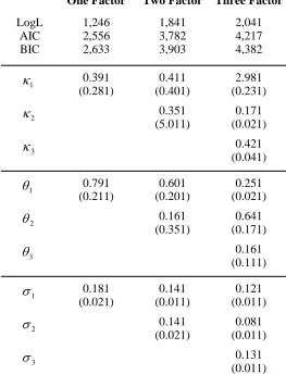
Table 1

Parameter Estimates, for the One, Two and Three-factor models (Apr-96 to

Mar-03)

The table shows the maximum-likelihood estimates for each of the three parameters {κ,θ,σ} of each factor, under the one, two, and three-factor models. The Log-likelihood calculations are based on

Equation (12), and used to calculate the Akaike Information Criterion (AIC), and Bayesian Information

Criterion (BIC). Standard errors based on the inverse Hessian matrix are shown below the parameter estimates.

One Factor Two Factor Three Factor

LogL 1,246 1,841 2,041 AIC 2,556 3,782 4,217 BIC 2,633 3,903 4,382

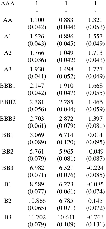
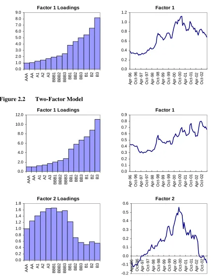
Table 2

Estimated Factor Loadings for the Three-Factor Model Apr-96 to Mar-03

Each of the 14 observed yield spread series by rating (AAA to B3) is expressed as a linear

combination of three factors, weighted by factor loadings. The j-th observed series at

time t is given by where is the sensitivity of the j-th

observed series to the i-th factor. The factor loadings shown in the table are the elements of

the measurement matrix from Equation (3). The first series (AAA) is assumed

equal to the simple sum of the three factors while factor loadings for the remaining series

are estimated by the maximum likelihood method. Standard errors are based on the

finite-difference Hessian matrix and shown below each loading estimate.

jt

Factor 1 Factor 2 Factor 3

AAA 1 1 1 - -

-AA 1.100 0.883 1.321 (0.042) (0.044) (0.053) A1 1.526 0.886 1.557

(0.043) (0.045) (0.049) A2 1.766 1.049 1.713

(0.036) (0.042) (0.043)

A3 1.930 1.498 1.727 (0.041) (0.052) (0.049) BBB1 2.147 1.910 1.668

(0.042) (0.047) (0.055) BBB2 2.381 2.285 1.466

(0.056) (0.044) (0.059)

BBB3 2.703 2.872 1.397 (0.061) (0.079) (0.081) BB1 3.069 6.714 0.014

(0.089) (0.120) (0.095) BB2 5.761 5.965 -0.049

(0.079) (0.081) (0.087) BB3 6.982 6.521 -0.224

(0.071) (0.076) (0.085) B1 8.589 6.273 -0.085

(0.077) (0.061) (0.074) B2 10.866 6.785 0.145

(0.065) (0.071) (0.072) B3 11.702 10.641 -0.763

Figure 2

Estimates of Factor Loadings and Factor Realizations for

Apr-96

to

Mar-03

Figure 2.1

One-Factor Model

Factor 1 Loadings

Figure 2.2

Two-Factor Model

Figure 3

Factors of the Three-Factor Model and Macroeconomic Variables:

Apr-96 to Mar-03

Factor 1 and the VIX

0

Factor 2 and the Long Bond Rate

0.0

Factor 3 and the S&P500

Figure 4

Conditional Density Log-Likelihoods for the One, Two, and Three-Factor

Model: Apr-96 to Mar-03

-15 -10 -5 0 5 10 15 20 25 30 35

Ap

r-96

Aug

-96

Dec-96 Ap

r-97

Aug

-97

Dec-97 Ap

r-98

Aug

-98

Dec-98 Ap

r-99

Aug

-99

Dec-99 Ap

r-00

Aug

-00

Dec-00 Ap

r-01

Aug

-01

Dec-01 Ap

r-02

Aug

-02

Dec-02

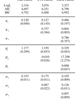
Table 3

Parameter Estimates, for the One, Two and Three-factor models (Apr-96 to

Mar-08)

The table shows the maximum-likelihood estimates for each of the three parameters {κ,θ,σ} of each factor, under the one, two, and three-factor models. The Log-likelihood calculations are based on

Equation (12), and used to calculate the Akaike Information Criterion (AIC), and Bayesian Information

Criterion (BIC). Standard errors based on the inverse Hessian matrix are shown below the parameter estimates.

One Factor Two Factor Three Factor

LogL 2,316 3,076 3,327 AIC 4,697 6,251 6,790 BIC 4,792 6,400 6,992

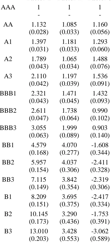
Table 4

Estimated Factor Loadings for the Three-Factor Model Apr-96 to Mar-08

Each of the 14 observed yield spread series by rating (AAA to B3) is expressed as a linear

combination of three factors, weighted by factor loadings. The j-th observed series at

time t is given by where is the sensitivity of the j-th

observed series to the i-th factor. The factor loadings shown in the table are the elements of

the measurement matrix from Equation (3). The first series (AAA) is assumed

equal to the simple sum of the three factors while factor loadings for the remaining series are estimated by the maximum likelihood method. Standard errors are based on the

finite-difference Hessian matrix and shown below each loading estimate.

jt

Factor 1 Factor 2 Factor 3

AAA 1 1 1 - - -AA 1.132 1.085 1.160

(0.028) (0.033) (0.056) A1 1.397 1.181 1.293

(0.031) (0.033) (0.060) A2 1.789 1.065 1.488

(0.043) (0.034) (0.076) A3 2.110 1.197 1.536

(0.042) (0.039) (0.091)

BBB1 2.321 1.471 1.432 (0.043) (0.045) (0.093) BBB2 2.611 1.738 0.990

(0.047) (0.064) (0.102) BBB3 3.055 1.999 0.903

(0.063) (0.089) (0.140)

BB1 4.579 4.070 -1.608 (0.168) (0.277) (0.344) BB2 5.957 4.037 -2.411

(0.154) (0.306) (0.328) BB3 7.115 3.842 -2.319

(0.149) (0.354) (0.306) B1 8.209 3.695 -2.417

(0.151) (0.375) (0.334) B2 10.145 3.290 -1.753

(0.173) (0.436) (0.391) B3 13.010 3.428 -3.062

(0.203) (0.553) (0.589)

Figure 5

Estimates of Factor Loadings and Factor Realizations for

Figure 5.1

One-Factor Model

Figure 5.2

Two-Factor Model

Figure 6

Estimated Factors of the Three-Factor Model and Macroeconomic

Variables: Apr-96 to Mar-08

Factor 1 and the VIX

0

Factor 2 and the Long Bond Rate

2

Factor 3 and S&P500

2

Figure 7

Conditional Density Log-Likelihoods for the One, Two, and Three-Factor

-10

-5 _{0 5} 10 15 20 25 30

Apr-96 Oct-96 Apr-97 Oct-97 Apr-98 Oct-98 Apr-99 Oct-99 Apr-00 Oct-00 Apr-01 Oct-01 Apr-02 Oct-02 Apr-03 Oct-03 Apr-04 Oct-04 Apr-05 Oct-05 Apr-06 Oct-06 Apr-07 Oct-07

One-Fac

tor

Tw

o-Factor

Three-Fac

tor

Figure 8

Measurement Error Variances

The figure shows the square roots of the estimated measurement error variances for each rating

series under the one, two, and three-factor model. The maximum-likelihood estimates are based on

the full period (Apr-96 to Mar-08), where the variances are the diagonal elements of matrix

in the Measurement Equation where . All variance

estimates are significant at the 5% level within each model. )

14 14 ( ×

H R_t =ZX_t+ε_t ε_t ~N(0,H)

Square Root of Estimated Measurement Error Variances for the One, Two and Three-Factor Model (in basis points)

0 20 40 60 80 100 120

AA

A

AA A1 A2 A3

B

BB1

B

BB2

B

BB3 BB1 BB2 BB3 B1 B2 B3

One Factor

Two Factor

Table 5

Credit Spread Summary Statistics and Model Fit Errors

The following table summarizes observed credit spreads for the 144 months from 30-Apr-96 to 31-Mar-08. For each month we calculate a vector of model fit errors, defined as the difference

between the 14 observed credit spreads and the fitted spreads defined by the

Measurement Equation (3) . The estimated state vector and measurement matrix

are based on the three-factor full period model. For each of the 14 credit spreads by

rating we generate a time-series of 144 fit error terms and calculate the average, standard deviation, and mean absolute percentage error (MAPE). We check and confirm that the calculated

standard deviations of errors are near-identical to the maximum-likelihood estimates of the square

roots of the measurement error variances (in Figure 8). )

Two Augmented Dickey-Fuller tests (ADF) are performed on each error time-series. The first

ADF test is based on an AR model with drift and the second is based on

the trend-stationary AR model

t

p-values show that the null hypothesis of a unit root φ= can be strongly rejected at the 5% significance level. The stationary error terms with averages close to zero suggest that the

multifactor Vasicek model provides an unbiased fit for credit spreads across ratings for the sample

period.

Index Avg (bp) SD (bp) Avg (bp) MAPE SD (bp) No Trend Trend

AAA 64.5 25.4 0.01 7.8% 5.7 <0.0001 <0.0001 AA 71.9 27.9 -0.02 5.3% 4.3 <0.0001 <0.0001 A1 83.9 31.3 -0.01 4.3% 4.1 <0.0001 0.0032 A2 94.7 33.7 0.14 2.9% 3.4 <0.0001 <0.0001 A3 108.9 38.4 0.30 3.5% 4.4 <0.0001 <0.0001

BBB1 123.3 40.8 -0.41 5.1% 7.3 0.0020 0.0126

BBB2 138.1 43.2 -0.77 6.2% 9.7 0.0075 0.0350

BBB3 159.9 47.9 -1.36 6.9% 13.0 0.0068 0.0522

BB1 247.1 96.5 4.25 9.5% 24.5 0.0045 0.0221

BB2 292.4 88.5 -0.13 2.5% 8.7 <0.0001 <0.0001 BB3 325.5 98.1 0.54 3.3% 12.8 <0.0001 <0.0001 B1 359.1 99.7 -1.19 2.8% 11.9 <0.0001 <0.0001 B2 415.0 119.6 -0.26 3.7% 19.6 <0.0001 <0.0001

B3 502.8 165.3 4.26 6.6% 39.5 0.0025 0.0112