SverigeS rikSbank
working paper SerieS
203
evaluating an estimated
new keynesian Small open
economy Model
Malin Adolfson, Stefan Laséen, Jesper Lindé
and Mattias Villani
working paperS are obtainable FroM
Sveriges riksbank • information riksbank • Se-103 37 Stockholm Fax international: +46 8 787 05 26
telephone international: +46 8 787 01 00 e-mail: [email protected]
the working paper series presents reports on matters in the sphere of activities of the riksbank that are considered
to be of interest to a wider public.
the papers are to be regarded as reports on ongoing studies and the authors will be pleased to receive comments.
the views expressed in working papers are solely the responsibility of the authors and should not to be interpreted as
Evaluating An Estimated New Keynesian Small Open Economy
Model
Malin Adolfson
Sveriges RiksbankStefan Laséen
Sveriges RiksbankJesper Lindé
Sveriges Riksbank and CEPRMattias Villani
∗Sveriges Riksbank and Stockholm University
Sveriges Riksbank Working Paper Series
No.
203
February 2007
Abstract
This paper estimates and tests a new Keynesian small open economy model in the tra-dition of Christiano, Eichenbaum, and Evans (2005) and Smets and Wouters (2003) using Bayesian estimation techniques on Swedish data. To account for the switch to an inflation targeting regime in 1993 we allow for a discrete break in the central bank’s instrument rule. A key equation in the model - the uncovered interest rate parity (UIP) condition - is well known to be rejected empirically. Therefore we explore the consequences of modifying the UIP condition to allow for a negative correlation between the risk premium and the expected change in the nominal exchange rate. The results show that the modification increases the persistence and volatility in the real exchange rate and that this model has an empirical advantage compared with the standard UIP specification.
Keywords: DSGE; VAR; VECM; Open economy; Bayesian inference.
JEL Classification Numbers: E17; C11; C53.
∗Address: Sveriges Riksbank, SE-103 37 Stockholm, Sweden. E-mails: [email protected],
1. Introduction
During the last years there has been a growing interest from academia and especially central banks in using dynamic stochastic general equilibrium (DSGE) models for analyzing macroeco-nomicfluctuations and to use these models for quantitative policy analysis. Smets and Wouters (2003,2004) have in a series of influential papers shown that the forecasting performance of the new generation of (closed economy) DSGE models in the tradition of Christiano, Eichenbaum and Evans (2005) compare very well with both standard and Bayesian vector autoregressive (VAR) models. Adolfson et al. (2005a) report similar results for an open economy DSGE model. However, even if these models appear to be able to capture the development of some key macroeconomic time series, there are still challenges to make them fulfill the observed properties in the data. Often the cross-equation restrictions implied by the DSGE model are simply too strict when taken to the data. One example is the inability of open economy models to account for the persistence and volatility in the real exchange rate, another is the failure of accounting for the international transmission of business cycles (see, e.g., Chari, Kehoe and McGrattan (2002); Lubik and Schorfheide, 2005; Justiniano and Preston (2005); de Walque, Smets and Wouters,
2005).
A key equation in open economy DSGE models is the uncovered interest rate parity (UIP) condition, which in its simplest formulation suggests that the difference between domestic and foreign nominal interest rates equals the expected future change in the nominal exchange rate. The UIP condition is a key equation in open economy models not only for the exchange rate but also for many macroeconomic variables, since there is a lot of internal propagation of exchange rate movements working throughfluctuating relative prices. There is, however, strong empirical evidence against the standard UIP condition. VAR evidence suggest that the impulse response function for the real exchange rate after a shock to monetary policy is hump-shaped with a peak effect after about 1 year (see, e.g., Eichenbaum and Evans, 1995; Faust and Rogers, 2003), whereas the standard UIP condition imply a peak effect within the quarter followed by a rela-tively quick mean reversion. Moreover, a DSGE model with a standard UIP condition cannot account for the so-called “forward premium puzzle” recorded in the data, i.e. that a currency whose interest rate is high tends to appreciate which implies that the risk premium must be negatively correlated with the expected exchange rate depreciation (see, e.g., Fama,1984; Froot and Frankel, 1989).
In an attempt to account for these empirical shortcomings, we alter the structural open economy DSGE model developed in Adolfson et al. (2005b) and modify the uncovered interest rate parity (UIP) condition to allow for a negative correlation between the risk premium and the expected change in the exchange rate, following the vast empirical evidence reported in for example Engel (1996). In the log-linearized version of the model, our suggested modification of the risk premium introduces a lagged dependence between the exchange rate and the domestic interest rate (which is absent using a standard UIP condition), and this may help the model to account for the hump-shaped impulse response functions to a policy shock found in VARs. To explore the quantitative role of the UIP condition in the model we make a thorough analysis of the empirical performance of the model with the standard and modified UIP condition for a set of key aggregate quantities and prices along a number of dimensions.
Sweden went from a fixed to a floating exchange rate and adopted an inflation targeting regime in the mid 90’s. We therefore believe that there are good reasons to allow for a change in the conduct of monetary policy before and after this event when estimating the model. The Riksbank abandoned the fixed exchange rate regime in November 1992 after the turmoil in the foreign exchange markets, and adopted a 2 percent inflation target in January 1993. The direction of monetary policy did consequently change in thefirst half of the 1990s and to formally take this into account in the model we allow the central bank to behave differently before and after the regime shift.1
By comparing impulse response functions and Bayesian posterior model probabilities we show that our specification allowing for a modified UIP condition better matches the observed properties of Swedish data relative to the model using a standard UIP condition. In addition, we examine the forecasting accuracy of the two DSGE specifications using a traditional out-of-sample rolling forecast evaluation for the period 1999Q1 to2004Q4. We contrast the forecasts from the alternative DSGE models to forecasts from both standard and Bayesian VAR models as well as traditional benchmark models such as the random walk, to get a better sense of the (relative) precision in the DSGE. Again we conclude that our DSGE specification with a regime shift and the modified UIP condition compares relatively well to more traditional forecasting tools. Lastly, we also use the approach in Del Negro and Schorfheide (2004) and Del Negro, Schorfheide, Smets and Wouters (2006) to learn more about the misspecification in each particular DSGE model, by exploiting the DSGE as a prior for a VAR model. If a particular DSGE prior is overruled by the data when estimating the VAR this questions the theoretical restrictions included in the DSGE model and indicates misspecification. Our results indicate that our open economy DSGE model’s theoretical restrictions are in fact useful for structuring reduced form VARs. However, even our relatively large model appears to be misspecified in the sense that a prior which is more loosely centered around the DSGE model is preferred in terms of the marginal likelihood. This is in line with the findings of Del Negro, Schorfheide, Smets and Wouters (2006).
The remainder of the paper is organized as follows. In Section 2, we briefly describe the theoretical open economy DSGE model. In Section 3 we discuss the data and the prior distri-butions used in the estimation. We also describe how to form a prior on the VAR from the DSGE model, and discuss how the (optimal) sharpness in this prior can help us characterize the degree of misspecification in our structural model. Section 4 contains the empirical results. We present the parameter estimates in the different DSGE specifications and compare the Bayesian posterior model probabilities. In addition, we report the forecasting accuracy of the two DSGE models and relate this to the forecasts from a Bayesian and a standard VAR. Subsequently we present the empirical results from the hybrid DSGE-VAR models, evaluating the degree of misspecification. Lastly, Section 6 provides some conclusions.
1The behavior of monetary policy in the in
2. The DSGE model
2.1. Model overview
This section gives an overview of the model economy and presents the key equations in the theoretical model.
The model is an open economy DSGE model very similar to the one developed in Adolfson et al. (2005b) and shares its basic closed economy features with many recent new Keynesian models, including the benchmark models of Christiano, Eichenbaum and Evans (2005), Altig, Christiano, Eichenbaum and Lindé (2003), and Smets and Wouters (2003).
The model economy consist of households, domestic goods firms, importing consumption and investment firms, exportingfirms, a government, a central bank, and an exogenous foreign economy. The households consume a basket consisting of domestically produced goods and imported goods, which are supplied by domestic and importing firms, respectively. We allow the imported goods to enter both aggregate consumption as well as aggregate investment. This is needed when matching the joint dynamics in both imports and consumption since imports (and investment) are much more volatile than consumption.
Households can invest in their stock of capital, save in domestic bonds and/or foreign bonds and hold cash. The choice between domestic and foreign bonds balances into an arbitrage condition pinning down expected exchange rate changes (i.e., an uncovered interest rate parity condition). Compared to a standard setting the risk premium is allowed to be negatively cor-related with the expected change in the exchange rate, following the evidence discussed in for example Duarte and Stockman (2005). As in the closed economy model households rent capital to the domesticfirms and decide how much to invest in the capital stock given costs of adjusting the investment rate. Wage stickiness is introduced through an indexation variant of the Calvo (1983) model.
Domestic production is exposed to stochastic unit root technology growth as in Altig et al. (2003). The firms (domestic, importing and exporting) all produce differentiated goods and set prices according to an indexation variant of the Calvo model. By including nominal rigidities in the importing and exporting sectors we allow for short-run incomplete exchange rate pass-through to both import and export prices.
Monetary policy is approximated with both a fixed exchange rate rule and a Taylor-type interest rate rule in which we allow for different monetary policy conduct before and after the adoption of an inflation targeting regime.
The model adopts a small open economy perspective where we assume that the foreign economy is exogenous. The foreign inflation, output and interest rate are therefore given by an exogenous VAR. In what follows we provide the optimization problems of the differentfirms and the households, and describe the behavior of the central bank.
2.2. Model
The model economy includes four different categories of operating firms. These are domestic goods firms, importing consumption, importing investment, and exporting firms, respectively. Within each category there is a continuum of firms that each produces a differentiated good. The domestic goodsfirms produce their goods using capital and labor inputs, and sell them to a retailer which transforms the intermediate products into a homogenous final good that in turn is sold to the households.
by a different firm, which follows the constant elasticity of substitution (CES) function
where λdt is a stochastic process that determines the time-varying flexible-price markup in the domestic goods market. The demand for firm i’s differentiated product, Yi,t, follows
Yi,t=
The production function for intermediate good iis given by
Yi,t=zt1−α tKi,tαHi,t1−α−ztφ, (3)
where zt is a unit-root technology shock common to the domestic and foreign economies, t is a domestic covariance stationary technology shock, Ki,t the capital stock and Hi,t denotes homogeneous labor hired by theithfirm. Afixed costz
tφis included in the production function. We set this parameter so that profits are zero in steady state, following Christiano et al. (2005). We allow for working capital by assuming that a fraction ν of the intermediatefirms’ wage bill has to befinanced in advance through loans from afinancial intermediary. Cost minimization yields the following nominal marginal cost for intermediatefirm i:
M Ctd= 1
whereRkt is the gross nominal rental rate per unit of capital,Rt−1 the gross nominal (economy
wide) interest rate, and Wt the nominal wage rate per unit of aggregate, homogeneous, labor
Hi,t.
Each of the domestic goodsfirms is subject to price stickiness through an indexation variant of the Calvo (1983) model. Since we have a time-varying inflation target in the model we allow for partial indexation to the current inflation target, but also to last period’s inflation rate in order to allow for a lagged pricing term in the Phillips curve. Each intermediate firm faces in any period a probability (1−ξd) that it can reoptimize its price. The reoptimized price is denoted Ptd,new.2 The differentfirms maximize profits taking into account that there might not be a chance to optimally change the price in the future. Firm i therefore faces the following optimization problem when setting its price
max conditional upon utility. βis the discount factor, andυt+sthe marginal utility of the households’ nominal income in periodt+s, which is exogenous to the intermediatefirms. πdt denotes inflation
in the domestic sector, ¯πct a time-varying inflation target of the central bank and M Ci,td the nominal marginal cost.
The first order condition of the profit maximization problem in equation (5) yields the following log-linearized Phillips curve:
³
We now turn to the import and export sectors. There is a continuum of importing consump-tion and investmentfirms that each buys a homogenous good at price Pt∗ in the world market, and converts it into a differentiated good through a brand naming technology. The exporting
firms buy the (homogenous) domestic final good at price Pd
t and turn this into a differentiated export good through the same type of brand naming. The nominal marginal cost of the im-porting and exim-porting firms are thus StPt∗ and Ptd/St, respectively, where St is the nominal exchange rate (domestic currency per unit of foreign currency). The differentiated import and export goods are subsequently aggregated by an import consumption, import investment and export packer, respectively, so that thefinal import consumption, import investment, and export good is each a CES composite according to the following:
Ctm = consumption (mc), import investment (mi) and export (x) sector. By assumption the continuum of consumption and investment importers invoice in the domestic currency and exporters in the foreign currency. In order to allow for short-run incomplete exchange rate pass-through to import as well as export prices we therefore introduce nominal rigidities in the local currency price, following for example Smets and Wouters (2002).3 This is modeled through the same type of Calvo setup as above. The price setting problems of the importing and exporting firms are completely analogous to that of the domesticfirms in equation (5), and the demand for the differentiated import and export goods follow similar expressions as to equation (2). In total there are thus four specific Phillips curve relations determining inflation in the domestic, import consumption, import investment and export sectors.
In the model economy there is also a continuum of households which attain utility from consumption, leisure and real cash balances. The preferences of householdj are given by
Ej0
where Cj,t,hj,t and Qj,t/Ptd denote the jth household’s levels of aggregate consumption, labor supply and real cash holdings, respectively. Consumption is subject to habit formation through
3There would be complete pass-through in the absence of nominal rigidities, since there are neither distribution
bCj,t−1, such that the household’s marginal utility of consumption is increasing in the quantity
of goods consumed last period. ζct and ζht are persistent preference shocks to consumption and labor supply, respectively. To make cash balances in equation (8) stationary when the economy is growing they are scaled by the unit root technology shock zt. Households consume a basket of domestically produced goods and imported products which are supplied by the domestic and importing consumption firms, respectively. Aggregate consumption is assumed to be given by the following constant elasticity of substitution (CES) function:
Ct=
where Ctd and Ctm are consumption of the domestic and imported good, respectively. ωc is the share of imports in consumption, and ηc is the elasticity of substitution across consumption goods.
The households invest in a basket of domestic and imported investment goods to form the capital stock, and decide how much capital to rent to the domesticfirms given costs of adjusting the investment rate. The households can increase their capital stock by investing in additional physical capital (It), taking one period to come in action. The capital accumulation equation is given by
whereS˜(It/It−1) determines the investment adjustment costs through the estimated parameter
˜
S00, andΥtis a stationary investment-specific technology shock. Total investment is assumed to be given by a CES aggregate of domestic and imported investment goods (Itd and Itm, respec-tively) according to
where ωi is the share of imports in investment, and ηi is the elasticity of substitution across investment goods.
Further, along the lines of Erceg, Henderson and Levin (2000), each household is a monopoly supplier of a differentiated labor service which implies that they can set their own wage. After having set their wage, households supply the firms’ demand for labor at the going wage rate. Each household sells its labor to a firm which transforms household labor into a homogenous good that is demanded by each of the domestic goods producing firms. Wage stickiness is introduced through the Calvo (1983) setup, where household j reoptimizes its nominal wage rate Wj,tnew according to the following
max
where ξw is the probability that a household is not allowed to reoptimize its wage, τyt a labor income tax, τwt a pay-roll tax (paid for simplicity by the households), andμz,t=zt/zt−1 is the
growth rate of the permanent technology level.4
4
For the households that are not allowed to reoptimize, the indexation scheme is Wj,t+1 =
(πc
The choice between domestic and foreign bond holdings balances into an arbitrage condition pinning down expected exchange rate changes (i.e., an uncovered interest rate parity condition). To ensure a well-defined steady-state in the model, we assume that there is premium on the foreign bond holdings which depends on the aggregate net foreign asset position of the domestic households, following, e.g., Lundvik (1992), and Schmitt-Grohé and Uribe (2001). A common problem with open economy DSGE models is that they typically do not provide enough persis-tence to generate a hump-shaped response of the real exchange rate after a shock to monetary policy, which is commonly found in estimated VARs (see, e.g., Eichenbaum and Evans, 1995; Faust and Rogers,2003). A novel feature with our specification of the risk premium is the inclu-sion of the expected change in the exchange rateEtSt+1/St−1. This is based on the observation
that risk premia are strongly negatively correlated with the expected change in the exchange rate (i.e., the expected depreciation), see e.g. Duarte and Stockman (2005) and Fama (1984). This pattern is often referred to as the “forward premium puzzle”. The risk premium is given by:
Φ(at, St,φ˜t) = exp
µ
−φ˜a(at−¯a)−˜φs
µ
EtSt+1 St
St
St−1 −
1 
+ ˜φt
, (13)
whereat≡(StBt∗)/(Ptzt)is the net foreign asset position, and˜φtis a shock to the risk premium. Consistent with the empirical evidence the idea here is that the domestic investors will require a lower expected return on their foreign bond holdings relative to their domestic deposits if the future exchange rate is easier to predict (that is, if the exchange rate is expected to depreciate consecutively). However, this formulation is not structural in the sense that such a risk pre-mium can be associated with the utility function in (8) or any standard utility function for a representative agent (see Backus, Foresi and Telmer, 2001, for a discussion). The UIP condition in its log-linearized form is given by:
b
Rt−Rb∗t =
³
1−φes´Et∆Sbt+1−eφs∆Sbt−φeabat+beφt, (14)
where∆is thefirst difference operator. By setting˜φs= 0we obtain the UIP condition typically used in small open economy models (see, e.g., Adolfson et al.,2005b). In the empirical analysis we formally test which specification is supported by the data.
Following Smets and Wouters (2003), monetary policy is approximated with a generalized Taylor (1993) rule. The central bank is assumed to adjust the short term interest rate in response to deviations of CPI inflation from the time-varying inflation target, the output gap (measured as actual minus trend output), the real exchange rate³xˆt≡Sˆt+ ˆPt∗−Pˆtc
´
and the interest rate set in the previous period. The instrument rule (expressed in log-linearized terms) follows:
b
Rt = ρR,tRbt−1+
¡
1−ρR,t¢ £bπ¯ct+rπ,t
¡ ˆ
πct−1−b¯πct¢+ry,tyˆt−1+rx,txˆt−1
¤
(15)
+r∆π,t∆πˆct+r∆y,t∆yˆt+εR,t,
during this sample period. Del Negro et al. (2006)find a similar result when estimating a closed economy DSGE model on US data.
Since Sweden went from a “fixed” to a floating exchange rate/inflation targeting regime in December 1992, we want to allow for a discrete break in the parameters to account for a policy regime shift. It is not obvious, however, how one should model policy prior to 1993Q1. Therefore, we study the empirical performance of three variants of the policy rule. In addition, results are also reported in the case where no break is allowed for, to see if the data support our prior that the policy rule has changed.5
The first specification is what will be referred to as a fixed exchange rate rule. It has the following structural form
b
Rt=rs∆Sˆt, (16)
where rs = 1,000,000, i.e. the interest rate will respond sharply to nominal exchange rate movements so as to keep it constant. Note that the reduced form associated with this formulation implies that the the interest rate will, for instance, respond one to one to foreign interest rate movements.6
The second specification is what will be referred to as a semi-fixed, or “target zone” rule following the ideas in Svensson (1994). This rule has essentially the same structure as(15)above but instead of responding to the real exchange rate, rs∆Sˆtis added to the rule with a high prior on rs. The prior value of rs is set so that the volatility of the nominal exchange rate in the model matches the exchange rate volatility in the data during the target-zone period (using the prior mode for the other parameters in the model).7
The third specification uses exactly the same formulation of the policy as in the inflation targeting period. Let θR,t collect the parameters of the monetary policy rule. We assume that
θR,t=
½
θR,1, if t <1993Q1 θR,2, if t≥1993Q1 ,
whereθR,1 captures the behavior of the central bank pre inflation targeting andθR,2captures the
behavior during the inflation targeting regime. There are mainly three reasons why we believe that a Taylor type rule may provide a good approximation of the conduct of monetary policy also before the adoption of an inflation target, when Sweden had afixed exchange rate. First, it should be recognized that the regime in practice was more of a managedfloat since the exchange rate was allowed to fluctuate within certain bands with recurring devaluations of the Krona.8
Second, there are writings published by the Riksbank which suggest that price stability was the overall objective even prior to the abandoning of thefixed exchange rate (Sveriges Riksbank Press
5
From 1977 to 1991, the Krona was pegged to a trade-weighted basket of 15 currencies of Sweden’s most important trading partners. The exchange rate was managed so as to allow limited fluctuations around the benchmark rate. However, the Krona was devalued 10% and 16% in 1981 and 1982, respectively. From mid-1991 the peg of the Swedish Krona was changed to a basket based on the European Currency Unit (ECU), with a
fluctuation range of plus or minus 1.5% of a central rate of SEK7.40054=ECU1.00.
6This rule abstracts from the two devaluations in 1981and 1982in the sense that the regime shift to the
Taylor-type inflation targeting rule in (15) only captures the adoption of afloating exchange rate in1993and the associated depreciation of the Krona. However, we only use the period1980Q1−1985Q4to form a prior on the unobserved state and not for inference.
7
Curdia and Finocchario (2005) use a similar rule, but assume that the Riksbank responded to exchange rate deviations from central parity instead.
8It could also be argued that the in
release 5/1993). However, third and finally, the Riksbank was not an independent institution during this period, and the interest rate setting were most likely influenced by policy makers, with a clear preference for output (employment) stabilization. For these reasons, the private sector’s perception of the actual policy rule in place on which they base their decision rules -could have been very different to that of the simple fixed exchange rate rule given by(16). We nevertheless let the data determine which one of these policy specifications are most preferred. When modelling the break in policy conduct, there is a need to take a stance on whether it was unanticipated or not. To simplify the analysis, we assume (i) that the break is completely unexpected and that (ii) once it had occurred, the new policy rule is assumed to be fully credible.9 The structural shock processes in the model is given in log-linearized form by the univariate representation
ˆςt=ρςˆςt−1+ες,t, ες,tiid∼N¡0, σ2ς
¢
(17)
whereςt={μz,t, t, λtj, ζct, ζht,Υt,φ˜t, εR,t,π¯ct,z˜t∗} andj ={d, mc, mi, x}.
The government spends resources on consuming part of the domestic good, and collects taxes from the households. The resultingfiscal surplus/deficit plus the seigniorage are assumed to be transferred back to the households in a lump sum fashion. Consequently, there is no government debt. Thefiscal policy variables - taxes on labor income, consumption, and the pay-roll, together with (HP-detrended) government expenditures - are assumed to follow an identified VAR model with two lags.
To simplify the analysis we adopt the assumption that the foreign prices, output (HP-detrended) and interest rate are exogenously given by an identified VAR model with four lags. Both the foreign and the fiscal VAR models are being estimated, using uninformative priors, ahead of estimating the structural parameters in the DSGE model.10
To clear the final goods market, the foreign bond market, and the loan market for working capital, the following three constraints must hold in equilibrium:
Ctd+Itd+Gt+Ctx+Itx≤zt1−α tKtαHt1−α−ztφ, (18)
StBt∗+1=StPtx(Ctx+Itx)−StPt∗(Ctm+Itm) +R∗t−1Φ(at−1,eφt−1)StBt∗, (19)
νWtHt=μtMt−Qt, (20)
whereGtis government expenditures,Ctx andItxare the foreign demand for export goods which follow CES aggregates with elasticity ηf, and μt = Mt+1/Mt is the monetary injection by the central bank. When defining the demand for export goods, we introduce a stationary asymmetric (or foreign) technology shockz˜t∗=zt∗/zt, wherezt∗ is the permanent technology level abroad, to allow for temporary differences in permanent technological progress domestically and abroad.
9For the
first and second formulation of the policy rule, we allow the agents to change their state variables according to the decision rules pertaining to the inflation targeting regime already from1992Q3(i.e. two quarters prior to the regime shift) in an attempt to improve the empirical performance of those two rules. The reason is that there were considerablefinancial turmoil in the Swedish exchange rate markets during this quarter. Among other things, the Riksbank raised the over-night interest rate to500percent (annualized rate) during this quarter in order to defend the Swedish Krona.
1 0The reason why we include foreign output HP-detrended and not in growth rates in the VAR is that the
To compute the equilibrium decision rules, we proceed as follows. First, we stationarize all quantities determined in period t by scaling with the unit root technology shockzt. Then, we log-linearize the model around the constant steady state and calculate a numerical (reduced form) solution with the AIM algorithm developed by Anderson and Moore (1985).
3. Estimation
3.1. Estimating the DSGE model
We start the empirical analysis by estimating the DSGE model, using a Bayesian approach and placing a prior distribution on the structural parameters. To estimate the model we use quarterly Swedish data for the period 1980Q1−2004Q4. All data were taken from Statistics Sweden, except the repo rate which were taken from Sveriges Riksbank. The nominal wage is taken from Statistics Sweden’s short term wage and salary statistics11 and is deflated by the
GDP deflator. The foreign variables on output, the interest rate and inflation are weighted together across Sweden’s 20 largest trading partners in 1991 using weights from the IMF.12
We include a large set of variables in the observed data vector, and match the following 15 variables: the GDP deflator, the real wage, consumption, investment, the real exchange rate, the short-run interest rate, hours worked, GDP, exports, imports, the consumer price index (CPI), the investment deflator, foreign output, foreign inflation and the foreign interest rate. As in Altig et al. (2003), the unit root technology shock induces a common stochastic trend in the real variables of the model. To make these variables stationary we use first differences and derive the state space representation for the following vector of observed variables
˜
Yt= [ π d
t ∆ln(Wt/Pt) ∆lnCt ∆lnIt xˆt Rt Hˆt ∆lnYt...
∆ln ˜Xt ∆ln ˜Mt πcpit πdef,it ∆lnYt∗ π∗t Rt∗ ]0.
. (21)
The growth rates are computed as quarter to quarter log-differences, while the inflation and interest rate series are measured as annualized quarterly rates. It should be noted that the stationary variablesxˆtandHˆtare measured as deviations around the mean, i.e. xˆt= (xt−x)/x and Hˆt= (Ht−H)/H, respectively. We choose to work with per capita hours worked, rather than total hours worked, because this is the object that appears in most general equilibrium business cycle models.13
In comparison with prior literature, such as for example Justiniano and Preston (2004) and Lubik and Schorfheide (2005), we have chosen to work with a large number of variables in order to facilitate identification of the parameters and shocks we estimate. For instance, despite the fact that the foreign variables are exogenous, we include them as observable variables as they enable identification of the asymmetric technology shock and are informative about the parameters governing the transmission of foreign impulses to the domestic economy. We estimate 13 structural shocks (see equation (17)) where 5 are assumed to be identically independently
1 1The wage series for the
first part of our sample is compiled by Friberg (2006).
1 2
The shares of import and export to output are increasing from about0.25 to 0.40 and from 0.21to 0.50
respectively during the sample period. In the model, import and export are however assumed to grow at the same rate as output. Hence, we decided to remove the excess trend in import and export in the data, to make the export and import shares stationary. For all other variables we use the actual series (seasonally adjusted with the X12-method except the variables in the GDP identity which were seasonally adjusted by Statistics Sweden).
1 3We used working age population to generate hours per capita. See Christiano, Eichenbaum and Vigfusson
distributed.14 In addition to these there are eight shocks provided by the exogenous (pre-estimated) fiscal and foreign VARs, whose parameters are kept fixed at their posterior mean estimates throughout the estimation of the DSGE model parameters. The shocks enter in such a way that there is no stochastic singularity in the likelihood function.15 To compute the likelihood function, the reduced form solution of the model is transformed into a state-space representation mapping the unobserved state variables into the observed data. We apply the Kalman filter to calculate the likelihood function of the observed variables, where the period 1980Q1-1985Q4 is used to form a prior on the unobserved state variables in 1985Q4 and the period 1986Q1-2004Q4 for inference.
The joint posterior distribution of all estimated parameters is obtained in two steps. First, the posterior mode and Hessian matrix evaluated at the mode is computed by standard numerical optimization routines. Second, the Hessian matrix is used in the Metropolis-Hastings algorithm to generate a sample from the posterior distribution (see Smets and Wouters (2003), and the references therein, for details). The results reported are based on a sample of 500,000 post burn-in draws from the posterior distribution.
We choose to calibrate those parameters which we think are weakly identified by the variables that we include in the vector of observed data. These parameters are mostly related to the steady-state values of the observed variables (i.e., the great ratios: C/Y,I/Y andG/Y).16 An alternative approach could be to include these parameters in the estimation. However, such a strategy would require a different set of variables to ensure proper identification, or conditioning the likelihood on the initial levels of the ratios, but would not yield different results since these parameters would simply capture the sample mean of the great ratios.
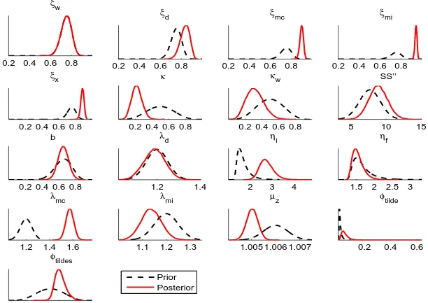
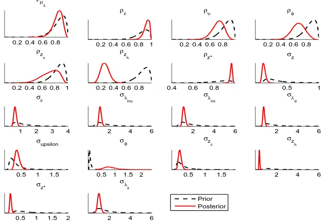
The parameters we choose to estimate pertain mostly to the nominal and real frictions in the model as well as the exogenous shock processes. Table 1 shows the assumptions for the prior distribution of the estimated parameters. The location of the prior distribution of the 43(51) estimated parameters with no break (break) in the monetary policy rule corresponds to a large extent to those in Adolfson et al. (2005b) on Euro area data. There are, however, some important differences in the choice of prior distribution to take notice of. First, the priors on the price stickiness parameters are chosen based on survey evidence on the frequency of price changes from a large number of Swedish firms. Apel, Friberg and Hallsten (2005) report that prices in Swedishfirms adjust only infrequently; the median firm adjusts the price once a year. Hence, the price and wage stickiness parameters are set so that the average length between price
1 4The shocks that are assumed to be iid are the monetary policy shock, the markup shock in the domestic
goods market, as well as the markup shocks the importing consumption, importing investment and exporting goods markets.
1 5Even if there is no stochastic singularity in the model we include measurement errrors in the 12 domestic
variables, since we know that the data series used are not perfectly measured and at best only approximations of the ’true’ series. In particular it was hard to remove the seasonal variation in the series, and there are still spikes in for example the inflation series, perhaps due to changes in the collection of the data. The variance of the uncorrelated measurement errors is set to 0 for the foreign variables and the domestic interest rate, 0.1 percent for the real wage, consumption and output, and 0.2 percent for all the other variables. This implies that the fundamental shocks explain about 90-95% of the variation in most of the variables. The measurement errors capture some of the high frequency movements in the data but notfluctuations related to the business cycle. Note also that our estimation results are robust to changning the size of the measurement errors (see the Appendix).
1 6The calibrated parameters are set to the following: the money growth μ = 1.010445; the discount factor β = 0.999; the depreciation rate δ = 0.01; the capital share in productionα = 0.25; the share of imports in consumption and investment ωc = 0.40 and ωi = 0.70, respectively; the share of wage bill financed by loans
and wage adjustments is4quarters. Second, the prior mean for the standard error of the markup shocks are all set to 1. This is about three times the prior mean in Adolfson et al. (2005b). The choice is based on the fact that Sweden is a much smaller economy than the Euro area and is therefore presumably expected to be subject to larger markup shocks. This is consistent with the observation that not only domestic, but also import prices are substantially more volatile than what is observed for the Euro area.
We choose identical priors for the parameters in the monetary policy rule before and after the adoption of an inflation target in 1993Q1. This is a useful benchmark prior for communi-cating the results, and allows us to assess how parameters change between the regimes due to information in the data and not due to different priors.
3.2. Detecting model misspecification using a VAR with a DSGE prior
The main Bayesian tool for contrasting the empirical coherence of different DSGE models is the posterior distribution over the set of compared models, wherein the marginal likelihood enters as the most essential ingredient. Such a model comparison is of course only a relative one, however. It may very well be the case that all of the models under comparison are severely misspecified. One way to investigate this is to compare their marginal likelihoods to those of more flexible empirically oriented models, such as VARs (see e.g. Smets and Wouters, 2003). Bayesian model probabilities have great appeal, but there is no escaping from the fact that they are sensitive to the choice of prior. This sensitivity may not have dramatic effects when the models under consideration are similar, and the prior is elicited in essentially the same way. This is not the case in the DSGE versus VAR comparison, however, as the statistically oriented priors traditionally used for reduced form VARs (e.g. Litterman, 1986) are radically different from the micro-based economic priors in DSGE models.
Del Negro and Schorfheide (2004) introduce an interesting alternative way to assess the degree of misspecification in DSGE models using Bayesian techniques. Del Negro, Schorfheide, Smets and Wouters (2006) extends the Del Negro-Schorfheide approach and re-interpret it from a different view-point. The idea is to compare the marginal likelihood of the possibly misspecified DSGE model to that of a VAR with a prior centered on the same DSGE model with the tightness of the prior determined by a single scalar-valued parameterλ(for details see Appendix 2). The DSGE-based prior has the effect of pulling the unrestricted VAR estimates toward the subspace where the DSGE restrictions are satisfied. In the limit λ = ∞, the prior imposes the DSGE restrictions with probability one, and the VAR thus collapses to the (VAR approximation of the) DSGE model. Asλgets smaller the prior becomes increasingly less informative and the Bayesian estimates of the VAR coefficients approach the OLS estimates. Del Negro and Schorfheide (2004) suggest computing the marginal likelihood of the VAR with a DSGE-based prior for different choices of λand subsequentlyfind the optimalλ, which we denote byλˆ. A largeλˆ then means that the implied cross-equation restrictions from the DSGE model are highly compatible with the observed data. A λˆ on the lower end of the scale suggests a preference for a prior on the VAR with a minimal use of the DSGE restrictions, which therefore cast doubt on the empirical coherence of the DSGE model.
is a good idea to use the cross moments from the DSGE model in the formation of a prior, in the sense that such a prior agrees well with the likelihood function.
The estimated VAR model contains the 15 observed variables that are used in the DSGE estimation (see equation (21)), where non-stationary variables enter infirst differences. However, the unit root technology shock in the theoretical DSGE model induces a common stochastic trend in the levels of all real variables, which implies that the levels of the variables may contain information about the current state of the economy. We therefore also estimate a vector error correction model (VECM) with a DSGE-based prior, following Del Negro et al. (2006), by just adding the cointegrating relations of the DSGE model to the VAR.
Given that the DSGE model allows all the reduced form parameters to change as a result of the regime shift, even if only a subset of the structural parameters change (i.e., the conduct of monetary policy), the same must be true in the VAR/VECM model. We therefore allow for a potential break in all the VAR/VECM parameters (lag-polynominal and covariance matrix) in t = 1993Q1. However, the VAR parameters in the two regimes coincide in all dimensions except those related to the monetary policy change, which an unrestricted estimation of the VAR parameters would ignore. Here we center the prior on the DSGE model with a break in the monetary rule which takes this fact into account. It should also be noted that although it is straightforward to use different prior tightness on the DSGE cross restrictions in these two subperiods, we restrictλto be the same for allt.
4. Results
4.1. Parameter estimates and marginal likelihood comparison
In Table 1 we report the priors along with the posterior median and standard deviation for the parameters in the various model specifications with different policy rules. The first four posterior results pertain to the model with a “standard” UIP condition while the last column relate to the model with the modified UIP condition.
A clear message from Table 1 is that a fixed exchange rate rule during the first part of the sample1986Q1−1992Q4is not preferred by the data. The log marginal likelihoods clearly favor any of the other policy rules. Even a specification of the model without allowing for a break in the policy rule is preferable to the fixed exchange rate version. The no-break policy rule is also preferred to the the target zone specification which has a high prior value on the parameter multiplying the change in the nominal exchange rate (rs). For the target zone rule, we also notice that the obtained posterior value for rs is substantially lower than the prior value, so the data do not seem to be supportive of a strong exchange rate response in the policy rule.17
Moving to the third formulation of the policy rule using a Taylor type instrument rule with a discrete break, we see, however, that this more flexible specification of the rule during the first part of the sample induces a strong improvement in the log marginal likelihood compared to the no-break case. Our interpretation of these results is that there is clear evidence in favor of a break in the monetary policy conduct, but that the fixed-exchange rate/target zone versions of the policy rule are not empirically successful. Perhaps due to lack of credibility since the more
flexible rule with a larger role for output stabilization appears to be more empirically coherent. Turning to the “deep” parameters, wefind that they are similar in the different specifications of the model, the main exception being the degree of wage stickiness which is found to be
sub-1 7It should, however, be noted that the estimated target zone rule still keeps the nominal exchange rate within
a band of±2%. This is actually similar to what is obtained under the Taylor type rule with a break, and the
stantially lower using the fixed-exchange rate or target-zone rules. For the other specifications, the posterior of the wage stickiness parameter essentially equals the prior.18 For the two model
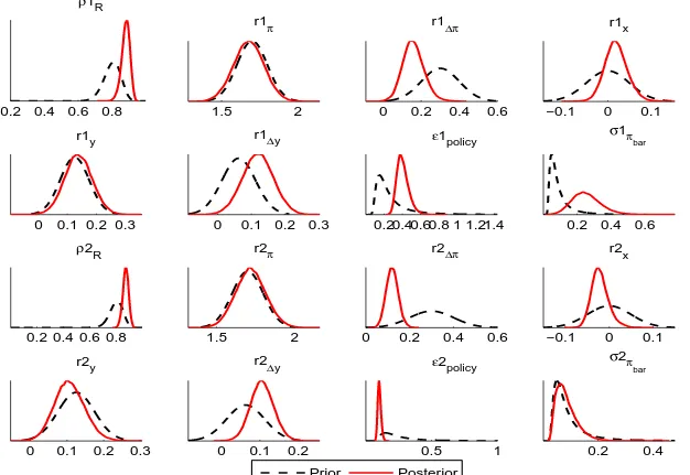
specifications using Taylor-type instrument rules, we see that the policy rule parameters are similar in the two regimes, with the exception of the estimated standard deviations of the infl a-tion target shock and the monetary policy shock which are considerably lower after the adopa-tion of an inflation target. Consequently, monetary policy in Sweden seems to have become more predictable after the adoption of an inflation target in1993. Notably, the posterior distribution for the coefficient on lagged inflation (rπ) in equation (15) is essentially identical to the prior distribution, suggesting weak identification of this parameter (see also Appendix 1) . However, by lowering and raising the prior mode and the standard deviation, we found that high values on this parameter is not favored by the Bayesian model probabilities but that values between 1.1-2 appear to be about equally plausible (given the other priors).19
We then go on to test the specification with the modified UIP condition. The idea is that the negative correlation between the risk premium and the expected change in the exchange rate via the UIP condition will affect the persistence in the real exchange rate after a contrac-tionary monetary policy shock. Looking at the parameter estimates in Table 1 we see that the persistence in the risk premium shock decreases in the specification with the modified UIP condition compared to the specification with a standard UIP condition. A lower persistence in the shock to the risk premium is now needed to capture the observed autocorrelation in the real exchange rate since the modified UIP condition induces endogenous inertia in the risk pre-mium through the negative correlation between the risk prepre-mium and the expected exchange rate change. While there is negative correlation between these parameters locally, it is very important to understand that the empirical relevance of these parameters for the entire model is identified by the fact that we evaluate the model’s empirical coherence on a number of variables in addition to the real exchange rate. Consequently the risk premium parameterφ˜sis identified separately from the risk-premium process parameters because the former parameter changes all shocks’ propagation to the other variables in the model via the exchange rate. To understand this mechanism we have conducted the following experiments.
First, we reestimated the model using uniform priors on both φ˜s and ρφ˜ and computed
the posterior median of φ˜s and ρ˜φ to be 0.67 and 0.48, respectively, which are in line with the results in Table 1. The associated log marginal likelihood is −2249.8, which is a slight improvement compared to the benchmark in Table 1 (−2252.5). Second, we calibrated φ˜s (ρ˜φ)
to zero, and reestimated the model using a uniform prior on ρ˜φ (φ˜s). The estimation outcome wasρ˜φ= 0.94(φ˜s= 0.79) and the log marginal likelihood−2269.9(−2256.8). While theφ˜sand
ρφ˜ parameters move somewhat in relation to the benchmark result to compensate for the missing
source of exchange rate persistence in these cases, it is clear from the associated log marginal likelihood values that the data support the existence of exchange rate persistence both through the modified UIP condition and through autocorrelated risk premium shocks. In particular, the drop in log marginal likelihood when omitting the modified risk premium is substantial, a finding in line with the key message of the paper. Third, we constructed contour plots of 1 8We have experimented with both a higher and a lower prior mode, as well as a uniform prior, on the wage
stickiness parameter, where the results indicate that the data is only weakly informative on this parameter (i.e., the posterior moves less than one-to-one with the prior). Since our prior belief is that wage stickiness is an important fricition we want to allow for uncertainty in the wage setting behavior, why we use an informative prior rather than calibrating this parameter.
1 9
the likelihood function in the n˜φs, ρ˜φ
o
-space conditional on the posterior median of the other
parameters (see Appendix 1). While we found some degree of substitutability betweenφ˜sandρφ˜
locally around the posterior mode (i.e., the likelihood is nearly constant in a neighborhood of the posterior mode), the likelihood is well shaped globally. However, dropping all observed variables except the real exchange rate in the measurement equation and drawing the same contour plots resulted in an ill-behaved corner solution (φ˜s= 1,ρφ˜ = 0). In conclusion, it is our belief that the
parameters in the modified version are well identified. This is also manifested by the difference in log marginal likelihoods, where the model with the modified UIP condition obtains a posterior probability of 1.0. The data thus indicate that there is in fact a negative correlation between the risk premium on foreign bonds and the expected exchange rate development in Sweden.
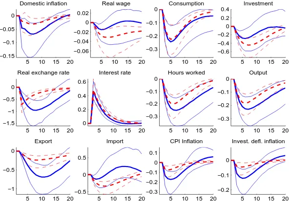
Figure 1 shows the impulse response functions after a one standard deviation shock to mon-etary policy with and without the modified UIP condition. The solid lines depict the median and 95% interval posterior responses in the specification with a modified UIP condition, and the dashed lines show the responses in the specification with a standard UIP condition. In either specification the contractionary shock has a gradual effect on both output and inflation, with a maximum impact in about 1 to 112 years which is in line with the ’conventional wisdom’ on the transmission of monetary policy originally stemming from VARs. The interest rate increase also makes the exchange rate appreciate directly, via the UIP condition. This in turn feeds into the import prices but not fully since prices are sticky which forces the exchange rate pass-through to be incomplete. Also domestic and export prices are affected to some extent through the marginal cost of imported inputs. In the specification including a standard UIP condition, the appreciation is immediate before the exchange rate gradually returns to its equilibrium value (dashed lines). However, in the model with the modified UIP condition the real exchange rate appreciates only slowly and gradually (solid lines), in contrast. The larger persistence in the modified UIP condition, through the lagged dependence between the exchange rate and the risk premium, turns the real exchange rate from a spiked to a hump-shaped response. The reason is that the new specification of the UIP condition, with a negative correlation between the risk premium and the expected exchange rate change, induces the households to require a lower risk adjusted expected return on their foreign investments relative to the remuneration on domestic bonds since the exchange rate is expected to depreciate in the future. But to then equalize the returns on the different bonds in the next period, the exchange rate necessarily has to appreciate even more in the forthcoming periods. Consequently, compared to the standard UIP specifi ca-tion the DSGE model with a modified UIP condition produces impulse response functions after an unexpected monetary policy shock that appear to come qualitatively closer what is observed in estimated VARs regarding the real exchange rate (see Adolfson et al., 2006 for evidence on Swedish data).
4.2. Forecasting performance
the random walk for the nominal exchange rate in terms of the forecasting precision (see, e.g., Meese and Rogoff,1983).
The forecast accuracy are assessed using a standard rolling forecast procedure where the models’ parameters are estimated up to a specified time period where the forecast distribution for the next 8 quarters subsequently is computed. The estimation sample is then extended to include one more (observed) data point, and the dynamic forecast distribution is computed for another 8 quarters. The forecasts are evaluated between 1999Q1 and 2004Q4 which gives 24
observations for the 1-step ahead forecast and16 observations for the 2-year ahead forecast. It should be noted that the VARs are re-estimated at this quarterly frequency while the DSGE models are re-estimated only yearly.
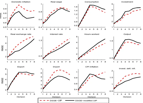
Figure2a shows the root mean squared forecast errors in percentage terms for the12domestic variables at 1 to 8 quarters horizon from the two alternative DSGE models with a standard UIP condition or the modified UIP condition, allowing for a policy regime shift in the Taylor type instrument rule. The forecast errors are calculated based on year-to-year forecasts for all variables except for the real exchange rate and hours worked which are measured as quarterly deviations from the steady-state.
By comparing the specifications with and without the modified UIP condition (solid and dashed lines, respectively) we see that the forecast accuracy in particular for the real exchange rate and the interest rate improves when the modified UIP condition is included in the model. The reason is that the low persistence in the standard UIP condition makes the real exchange return too rapidly to the steady state. Also the precision of the CPI inflation forecast increases at the medium to long-term horizons. On the other hand, the forecast accuracy of hours worked, output and investment are worse than in the specification with a standard UIP condition. Taken together, the joint forecasting precision (not shown) indicates that the two models perform equally well when accounting for all variables, while the model with the modified UIP condition has somewhat better accuracy when taking the forecasts of the subset of key macroeconomic variables, CPI inflation, output, interest rate, real exchange rate, exports and imports, into account.
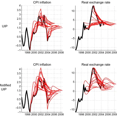
To get a sense for the precision of the forecasts we examine the actual forecasts from the two models using the standard UIP and the modified UIP conditions. Figure 3 shows the rolling forecasts for CPI inflation, the real exchange rate and the interest rate between 1999Q1 and
2004Q4from the standard and modified UIP specifications together with the actual outcomes. It is clear that the modified UIP enables the model to produce more persistent real exchange rate forecasts, while the mean reversion of the real exchange rate is a lot faster when using the standard UIP condition. It is also clear from Figure3that the shape of the forecasts for the CPI inflation and the interest rate are affected to a smaller extent. From a policy making perspective we believe that the model with the modified UIP is clearly preferable because it is unlikely that a central banker would like to use a model which always implies that the forecast path of the real exchange rate is quickly mean reverting no matter what.
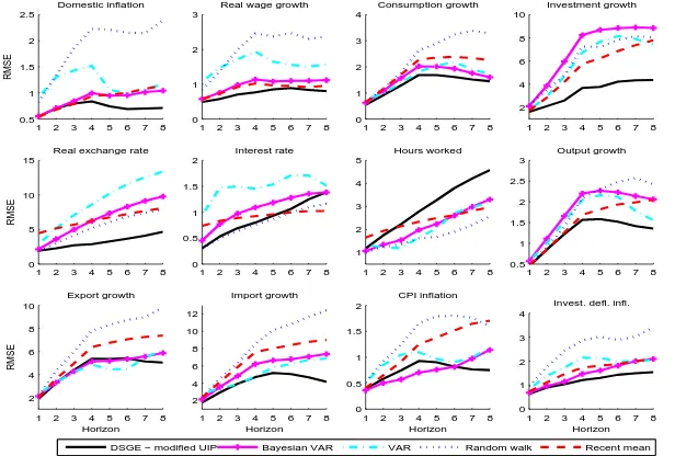
In Figure 2b we compare the DSGE model including the modified UIP condition with two VAR models (Bayesian and maximum likelihood estimates) and two naïve setups (random walks and the means of the eight most recent data observations).20 The DSGE model compares very
well to both the VAR and the BVAR for almost all variables. The exception is hours worked. The precision in both the output and the CPI inflation forecasts from the DSGE is line with the more empirically oriented VAR models, and at the two-year horizon they are in fact better. Especially interesting are the real exchange rate and interest rate forecasts where the DSGE
2 0It should be noted that the we are using an informative prior on the long-run mean in the BVAR such that the
model outperforms the two VARs at just about all horizons. In particular the real exchange rate forecasts from the DSGE does remarkably well and beats also the random walk as well as the means of the latest eight observations. More problematic is perhaps that the interest rate forecasts in the structural model is not able to surpass the random walk at any horizon. Nevertheless, taking the joint forecast precision of all variables into account, the DSGE model performs better than both the VAR and the BVAR at all horizons (not shown). The joint forecasts from the DSGE are more precise than joint forecasts from the VAR or the BVAR. Consequently, the DSGE model with a modified UIP condition appear to be the best forecasting tool out of the different models we compare.
4.3. Model misspecification
According to the Bayesian model posterior probabilities and the shape of the impulse response functions after a monetary policy shock we know that the DSGE specification including the modified UIP condition and allowing for changes in the policy rule is preferred by the data. However, as argued in Section 3.2, we still only know that this specification is preferred over the competing variants of the DSGE model; it may very well be the case that all of these models, including the winning specification, suffer from misspecification. Here we use the tools developed by Del Negro and Schorfheide (2004) and extended by Del Negro, Schorfheide, Smets and Wouters (2006) to gauge the degree of misspecification in a DSGE model by comparing its marginal likelihood to the marginal likelihood of a VAR with a prior centered on that particular DSGE model (see the Appendix for details).
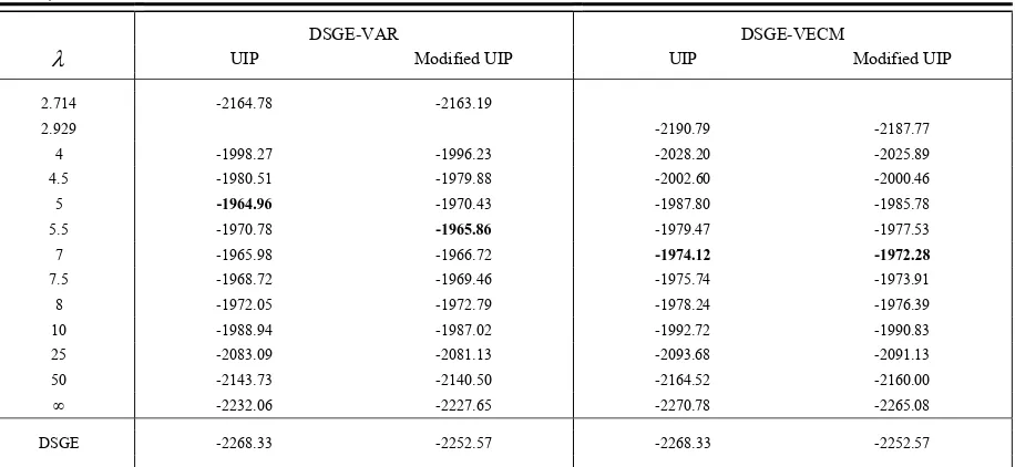
Table 2 reports the log marginal likelihoods when varying the tightness in the prior on the VAR/VECM model (λ) from very diffuse to more and more informative. Or in other words, when letting the cross-equation DSGE restrictions become more and more enforced in the VAR/VECM estimation. The table shows estimation results from the VAR and the VECM with a break in the parameters using the DSGE model with a Taylor-type instrument rule including a shift in the policy parameters as the prior. The VAR and the VECM are estimated using two different DSGE priors; the DSGE specification with a standard UIP condition and the DSGE specification including the modified UIP condition. By comparing the hybrid models’ marginal likelihoods when using these two DSGE priors we can examine the importance of the implied DSGE restrictions when taking possible misspecification of the DSGEs into account.
The results can be summarized as follows. First, according to the difference in marginal likelihoods between the structural DSGE model and the VAR/VECM approximations of the DSGE (i.e., λ=∞), the VECM provides a better approximation of the DSGE than the VAR. The reason is that the unit root technology shock in the theoretical DSGE model induces a common stochastic trend in the levels of all real variables, which makes the DSGE contain six cointegrating relations. Allowing the approximation to also hold cointegration vectors (which is done in the VECM but not in the VAR) therefore improves the marginal likelihood difference between the resulting hybrid model and the DSGE.21 Taken together we believe that the VECM approximation of the DSGE is satisfactory. As explained in Section 3.2 the analysis correctly identifies whether the DSGE is a useful prior also in the case with a less accurate approximation (which holds true for the VAR). However, as the approximation error increases it becomes more difficult to measure in which dimensions the cross-equation restrictions need to be relaxed since the DSGE model does not map well into the VAR in this case. For this reason we only use the
2 1Also a comparison of the autocovariance function of the DSGE-VAR and DSGE-VECM withλ=
VECM setup below when trying to assess in which dimensions the DSGE is misspecified. The optimal value of λ is around 5 in the VAR model and 7 in the VECM model. These numbers are much larger than those reported in Del Negro and Schorfheide (2004) (λˆ = 0.6) and Del Negro et al. (2006) (ˆλ= 0.75for the VAR andλˆ = 1for the VECM). It may seem as if the restrictions in our DSGE model compares favorably to previously studied models since the prior tightness λis a measure of prior concentration of the VAR prior around the DSGE cross moments. However, it should be noted that the optimal lambdas are not comparable across studies. The interpretation of the prior tightnessλis directly dependent on the model size and the size of the data set. One complicating circumstance is that we need λlarge enough for the prior to be proper, which is a necessary condition for computing meaningful marginal likelihoods. Part of the artificial DSGE observations that forms the prior (usually referred to as a training sample) is consumed in the process of turning the initially improper prior into a proper density (λmin), and is therefore not used in the actual model evaluation.22 One way to control for the
fact that λmin is dependent on the model and sample size is to report the marginal likelihood
as a function of the ratio of the number of post-training artificial observation to the number of actual observations, λ−λmin, or perhaps even better, the number of post-training artificial
observations and the size of the actual data.23
Table 2 also shows that the VECMs always have smaller marginal likelihood compared to the corresponding VARs. Irrespective of the choice of model and the size of λ, there is essentially zero posterior probability placed on the VECM compared to the VAR. This suggests that there is weak support in the data for the cointegration restrictions in the DSGE model. This result is more or less expected as graphs on the supposedly stationary cointegration relations reveal that at least some of them are on the borderline to non-stationarity (not shown here). Complementary evidence on this issue is given in Adolfson et al. (2005a) where it is reported that imposing cointegration restrictions in the estimation of a DSGE on Euro area data produces forecasts that are less accurate compared to when the model consistent cointegrating vectors are not imposed.
Turning to the comparison of the specifications with and without the modified UIP con-dition, we see in the VECM that the difference in marginal likelihood between the two UIP specifications is increasing when λ is increasing from its minimum value up to the (almost) DSGE approximating value of∞. For the VAR models the results are less clear. Given that the restrictions in the DSGE have more impact on the estimated VAR/VECM whenλis large, it is expected that the marginal likelihood difference will approach that of the two structural DSGEs as λ increases. In the DSGE approximating VECMs the difference between the standard and modified UIP specifications is 6 log units in favour of the modified condition. This should be compared with 15 log unit differences that are obtained for the structural DSGE. However, the Bayesian posterior model probabilities at the optimal λ (where the degree of sharpness in the DSGE prior maximizes the marginal likelihood) indicate that the difference in marginal likeli-hoods between the VAR/VECM specifications using the DSGE with or without the modified UIP condition is in fact relatively small.
One way to assess how much and in what dimensions the cross equation restrictions has
2 2The prior is proper ifλ ≥λ
min = [n(p+ 1) +q]/T,where n is the number of endogenous variables in the VAR withp lags,q the number of exogenous variables andT the number of actual data observations (see the Appendix for details). This is further complicated by the fact that we have a break in our model, which requires two training samples, one before and one after the regime shift. In our application we haven= 15endogenous variables in the VAR,p= 4lags andT = 48observations after the regime shift, so thatλminis close to 2.7, which clearly shows that this aspect is quite important for the interpretation of the results.
2 3For instance, the optimal number of post-training arti
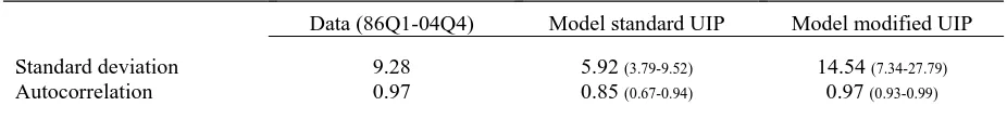
been relaxed is to compare the cross correlation functions forλ=∞ and λ=λb along with the standard deviations of the variables taken from the VECM covariance matrix. This is done in Figure 4. From thefigure we see that the differences in both autocorrelations and standard devi-ations are generally large both contemporaneously and over time, suggesting that bλ= 7implies a substantial relaxation of the DSGE’s cross equation restrictions on both the VAR polyno-mial and the covariance matrix. In particular the differences are large for real exchange rate’s autocorrelations and standard deviation, indicating that the model is still misspecified in this dimension even when including our modified UIP condition.24 It should, however, be
acknowl-edged that there is a great amount of uncertainty regarding the univariate point estimates of the correlations, but the improvement in log marginal likelihood for the hybrid model compared to the structural DSGE suggest that these differences are important when taken together.
5. Conclusions
In this paper we have tried to improve on a small open economy dynamic model in the new Keynesian tradition to make it comply better with the empirical evidence on the transmission mechanism of monetary policy and the forward discount puzzle. The former is especially im-portant for a policy making institution such as a central bank. Even if a DSGE model is able to capture the main development of the key macroeconomic time series and can forecast these well, one may also want to use the structural model for carrying out policy experiments such as evaluating alternative interest rate paths. It is then of crucial importance that the mechanisms in the model conform to the central bank’s view of the workings in the economy.
We have therefore addressed the common problem that open economy sticky price models where agents are allowed to freely trade in foreign and domestic bonds are typically not able to reproduce the observed persistence and volatility of the real exchange rate. This is troublesome when analyzing the effects of changes in monetary policy because the UIP condition is an integral part of determining how interest rate adjustments affect nominal and real exchange rates. The way the exchange rate responds to various shocks through the UIP condition is also important for many macroeconomic variables because of the nominal frictions in the model. Sticky prices increase the exchange rate’s effect on relative prices which in turn have an impact on most aggregate quantities and prices. To be able to generate intrinsic persistence of the exchange rate in the model, we introduced a negative correlation between the risk premium on foreign investments and the expected change in the exchange rate, following the empirical evidence in for example Engel (1996). Our tools to evaluate the modification empirically were Bayesian posterior model probabilities, impulse response functions, out-of-sample forecasts, and an analysis of the different DSGE restrictions’ empirical coherence by examining the suitability of the DSGEs as a prior for a VAR model.
We find that the modified UIP condition is strongly preferable to a standard specification according to the Bayesian posterior odds, and that it has a significant effect on the impulse response functions of a monetary policy shock. The transmission mechanism of monetary policy in the modified model is more in line with the results obtained from the identified VAR literature, in the sense that the effects on the real exchange rate becomes hump-shaped with a peak effect after year. The modified DSGE model also produces more accurate forecasts on the real exchange rate and the interest rate compared with a standard UIP specification. We therefore think it
2 4
References
Adolfson, Malin, Mikael K. Andersson, Jesper Lindé, Mattias Villani and Anders Vredin (2006), “Modern Forecasting Models in Action: Improving Macroeconomic Analyses at Central Banks”, Working Paper No. 188, Sveriges Riksbank.
Adolfson, Malin, Jesper Lindé and Mattias Villani (2005a), “Forecasting Performance of an Open Economy Dynamic Stochastic General Equilibrium Model”, Working Paper No. 190, Sveriges Riksbank.
Adolfson, Malin, Stefan Laséen, Jesper Lindé and Mattias Villani (2005b), “Bayesian Estimation of an Open Economy DSGE Model with Incomplete Pass-Through”, Working Paper No. 179, Sveriges Riksbank.
Altig, David, Lawrence Christiano, Martin Eichenbaum and Jesper Lindé (2003), “The Role of Monetary Policy in the Propagation of Technology Shocks”, manuscript, Northwestern University.
Anderson, Gary and George Moore (1985), “A Linear Algebraic Procedure for Solving Linear Perfect Foresight Models”, Economics Letters 17(3), 247-252.
Apel, Mikael, Richard Friberg and Kerstin Hallsten (2005), “Microfoundations of Macroeconomic Price Adjustment: Survey Evidence from Swedish Firms”, Journal of Money Credit and Banking 37, 313-338.
Backus, David, Silverio Foresi and Chris Telmer (2001), “Affine Term Structure Models and the Forward Premium Anomaly”, Journal of Finance 56 (1), 279-304.
Calvo, Guillermo (1983), ”Staggered Prices in a Utility Maximizing Framework”, Journal of Monetary Economics 12, 383-398.
Chari, , Patrick Kehoe and Ellen McGrattan (2002), “Can Sticky Price Models Generate Volatile and Persistent Real Exchange Rates?”, Review of Economic Studies 69, 533-563.
Christiano, Lawrence, Martin Eichenbaum and Charles Evans (2005), “Nominal Rigidities and the Dynamic Effects of a Shock to Monetary Policy”, Journal of Political Economy 113(1), 1-45.
Christiano, Lawrence, Martin Eichenbaum and Robert Vigfusson (2003), “What Happens After a Technology Shock?”, NBER Working Paper, No. 9819.
Curdia, Vasco and Daria Finocchiaro (2005), “An Estimated DSGE for Sweden with a Monetary Regime Change”, Seminar Paper No. 740, Institute for Intenational Economic Studies, Stockholm University.
Del Negro, Marco, Frank Schorfheide (2004), “Priors from General Equilibrium Models for VARS”, International Economic Review 45(2), 643-673.
Del Negro, Marco, Frank Schorfheide, Frank Smets and Raf Wouters (2006), “On the Fit and Forecasting Performance of New Keynesian Models”, Journal of Business and Economic Statistics, forthcoming.