Electromagnetics
Third Edition
6000 Broken Sound Parkway NW, Suite 300 Boca Raton, FL 33487-2742
© 2018 by Taylor & Francis Group, LLC
CRC Press is an imprint of Taylor & Francis Group, an Informa business No claim to original U.S. Government works
Printed on acid-free paper Version Date: 20180308
International Standard Book Number-13: 978-1-4987-9656-9 (Hardback)
This book contains information obtained from authentic and highly regarded sources. Reasonable efforts have been made to publish reliable data and information, but the author and publisher cannot assume responsibility for the validity of all materials or the consequences of their use. The authors and publishers have attempted to trace the copyright holders of all material reproduced in this publication and apologize to copyright holders if permission to publish in this form has not been obtained. If any copyright material has not been acknowledged please write and let us know so we may rectify in any future reprint.
Except as permitted under U.S. Copyright Law, no part of this book may be reprinted, reproduced, transmitted, or utilized in any form by any electronic, mechanical, or other means, now known or hereafter invented, including photocopying, microfilming, and recording, or in any information storage or retrieval system, without written permission from the publishers.
For permission to photocopy or use material electronically from this work, please access www.copyright.com (http://www.copyright.com/) or contact the Copyright Clearance Center, Inc. (CCC), 222 Rosewood Drive, Danvers, MA 01923, 978-750-8400. CCC is a not-for-profit organization that provides licenses and registration for a variety of users. For organizations that have been granted a photocopy license by the CCC, a separate system of payment has been arranged.
Trademark Notice: Product or corporate names may be trademarks or registered trademarks, and are used only for identification and explanation without intent to infringe.
Visit the eResources: https://www.crcpress.com/9781498796569 Visit the Taylor & Francis Web site at
Contents
Preface xxi
Authors xxv
1 Introductory concepts 1
1.1 Notation, conventions, and symbology . . . 1
1.2 The field concept of electromagnetics . . . 2
1.2.1 Historical perspective . . . 2
1.2.2 Formalization of field theory . . . 4
1.3 The sources of the electromagnetic field . . . 5
1.3.1 Macroscopic electromagnetics . . . 6
1.3.1.1 Macroscopic effects as averaged microscopic effects . . . 7
1.3.1.2 The macroscopic volume charge density . . . 7
1.3.1.3 The macroscopic volume current density . . . 10
1.3.2 Impressed vs. secondary sources . . . 11
1.3.3 Surface and line source densities . . . 12
1.3.4 Charge conservation . . . 15
1.3.4.1 The continuity equation . . . 16
1.3.4.2 The continuity equation in fewer dimensions . . . 18
1.3.5 Magnetic charge . . . 20
1.4 Problems . . . 21
2 Maxwell’s theory of electromagnetism 23 2.1 The postulate . . . 23
2.1.1 The Maxwell–Minkowski equations . . . 24
2.1.1.1 The interdependence of Maxwell’s equations . . . 25
2.1.1.2 Field vector terminology . . . 26
2.1.1.3 Invariance of Maxwell’s equations . . . 27
2.1.2 Connection to mechanics . . . 27
2.2 The well-posed nature of the postulate . . . 28
2.2.1 Uniqueness of solutions to Maxwell’s equations . . . 29
2.2.2 Constitutive relations . . . 31
2.2.2.1 Constitutive relations for fields in free space . . . 33
2.2.2.2 Constitutive relations in a linear isotropic material . . . 34
2.2.2.3 Constitutive relations for fields in perfect conductors . 36 2.2.2.4 Constitutive relations in a linear anisotropic material . 37 2.2.2.5 Constitutive relations for biisotropic materials . . . 38
2.2.2.6 Constitutive relations in nonlinear media . . . 40
2.3 Maxwell’s equations in moving frames . . . 41
2.3.1 Field conversions under Galilean transformation . . . 41
2.3.2 Field conversions under Lorentz transformation . . . 45
2.3.2.1 Lorentz invariants . . . 49
2.3.2.2 Derivation of Maxwell’s equations from Coulomb’s law 51 2.3.2.3 Transformation of constitutive relations . . . 51
2.3.2.4 Constitutive relations in deforming or rotating media . 53 2.4 The Maxwell–Boffi equations . . . 53
2.4.1 Equivalent polarization and magnetization sources . . . 55
2.4.2 Covariance of the Boffi form . . . 56
2.5 Large-scale form of Maxwell’s equations . . . 58
2.5.1 Surface moving with constant velocity . . . 59
2.5.1.1 Kinematic form of the large-scale Maxwell equations . . 61
2.5.1.2 Alternative form of the large-scale Maxwell equations . 64 2.5.2 Moving, deforming surfaces . . . 65
2.5.3 Large-scale form of the Boffi equations . . . 66
2.6 The nature of the four field quantities . . . 67
2.7 Maxwell’s equations with magnetic sources . . . 69
2.8 Boundary (jump) conditions . . . 71
2.8.1 Boundary conditions across a stationary, thin source layer . . . 71
2.8.2 Boundary conditions holding across a stationary layer of field discontinuity . . . 73
2.8.3 Boundary conditions at the surface of a perfect conductor . . . 77
2.8.4 Boundary conditions across a stationary layer of field discontinuity using equivalent sources . . . 77
2.8.5 Boundary conditions across a moving layer of field discontinuity . 78 2.9 Fundamental theorems . . . 79
2.9.1 Linearity . . . 79
2.9.2 Duality . . . 80
2.9.2.1 Duality of electric and magnetic point source fields . . 82
2.9.2.2 Duality in a source-free region . . . 83
2.9.3 Reciprocity . . . 84
2.9.4 Similitude . . . 85
2.9.5 Conservation theorems . . . 87
2.9.5.1 The system concept in the physical sciences . . . 87
2.9.5.2 Conservation of momentum and energy in mechanical systems . . . 88
2.9.5.3 Conservation in the electromagnetic subsystem . . . 91
2.9.5.4 Interpretation of the energy and momentum conserva-tion theorems . . . 94
2.9.5.5 Boundary conditions on the Poynting vector . . . 97
2.9.5.6 An alternative formulation of the conservation theorems 98 2.10 The wave nature of the electromagnetic field . . . 98
2.10.1 Electromagnetic waves . . . 99
2.10.2 Wave equation for bianisotropic materials . . . 102
2.10.3 Wave equation using equivalent sources . . . 105
2.10.4 Wave equation in a conducting medium . . . 105
2.10.4.1 Scalar wave equation for a conducting medium . . . 106
2.10.5 Fields determined by Maxwell’s equations vs. fields determined by the wave equation . . . 106
2.10.7 Propagation of cylindrical waves in a lossless medium . . . 114
2.10.8 Propagation of spherical waves in a lossless medium . . . 117
2.10.9 Energy radiated by sources . . . 120
2.10.10 Nonradiating sources . . . 122
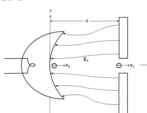
2.11 Application: single charged particle motion in static electric and magnetic fields . . . 124
2.11.1 Fundamental equations of motion . . . 124
2.11.2 Nonrelativistic particle motion in a uniform, static electric field . . 126
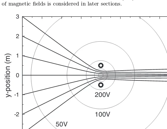
2.11.3 Nonrelativistic particle motion in a nonuniform, static electric field; electron optics . . . 130
2.11.4 Nonrelativistic particle motion in a uniform, static magnetic field 132 2.11.5 Nonrelativistic particle motion in uniform, static electric and magnetic fields: E×B drift . . . 138
2.11.6 Nonrelativistic particle motion in a nonuniform, static magnetic field . . . 141
2.11.7 Relativistic particle motion in a uniform, static magnetic field . . 142
2.11.8 Relativistic particle motion in uniform, static electric and magnetic fields . . . 142
2.12 Problems . . . 145
3 The static and quasistatic electromagnetic fields 151 3.1 Statics and quasistatics . . . 151
3.2 Static fields and steady currents . . . 151
3.2.1 Decoupling of the electric and magnetic fields . . . 152
3.2.2 Static field equilibrium and conductors . . . 153
3.2.3 Steady current . . . 155
3.3 Electrostatics . . . 158
3.3.1 Direct solutions to Gauss’s law . . . 158
3.3.2 The electrostatic potential and work . . . 160
3.3.2.1 The electrostatic potential . . . 160
3.3.3 Boundary conditions . . . 163
3.3.3.1 Boundary conditions for the electrostatic field . . . 163
3.3.3.2 Boundary conditions for steady electric current . . . 163
3.3.4 Uniqueness of the electrostatic field . . . 165
3.3.5 Poisson’s and Laplace’s equations . . . 166
3.3.5.1 Uniqueness of solution to Poisson’s equation . . . 167
3.3.5.2 Integral solution to Poisson’s equation: the static Green’s function . . . 167
3.3.5.3 Useful derivative identities . . . 169
3.3.5.4 The Green’s function for unbounded space . . . 171
3.3.5.5 Coulomb’s law . . . 171
3.3.5.6 Green’s function for unbounded space: two dimensions 172 3.3.5.7 Dirichlet and Neumann Green’s functions . . . 173
3.3.5.8 Reciprocity of the static Green’s function . . . 175
3.3.5.9 Image interpretation for solutions to Poisson’s equation 176 3.3.6 Force and energy . . . 181
3.3.6.1 Maxwell’s stress tensor . . . 181
3.3.6.2 Electrostatic stored energy . . . 182
3.3.7.1 Physical interpretation of the polarization vector in a
dielectric . . . 190
3.3.7.2 Potential of an azimuthally symmetric charged spheri-cal surface . . . 191
3.3.8 Field produced by a permanently polarized body . . . 192
3.3.9 Potential of a dipole layer . . . 193
3.3.10 Behavior of electric charge density near a conducting edge . . . . 196
3.3.11 Solution to Laplace’s equation for bodies immersed in an impressed field . . . 197
3.4 Magnetostatics . . . 199
3.4.1 Direct solutions to Ampere’s law . . . 200
3.4.2 The magnetic scalar potential . . . 202
3.4.3 The magnetic vector potential . . . 203
3.4.3.1 Integral solution for the vector potential . . . 205
3.4.3.2 Magnetic field of a small circular current loop . . . 208
3.4.4 Multipole expansion . . . 209
3.4.4.1 Physical interpretation ofMin a magnetic material . . 210
3.4.5 Boundary conditions for the magnetostatic field . . . 211
3.4.6 Uniqueness of the magnetostatic field . . . 212
3.4.6.1 Integral solution for the vector potential . . . 213
3.4.6.2 The Biot–Savart law . . . 215
3.4.7 Force and energy . . . 219
3.4.7.1 Ampere force on a system of currents . . . 219
3.4.7.2 Maxwell’s stress tensor . . . 221
3.4.7.3 Torque in a magnetostatic field . . . 222
3.4.7.4 Joule’s law . . . 224
3.4.7.5 Stored magnetic energy . . . 225
3.4.8 Magnetic field of a permanently magnetized body . . . 229
3.5 Static field theorems . . . 232
3.5.1 Mean value theorem of electrostatics . . . 232
3.5.2 Earnshaw’s theorem . . . 233
3.5.3 Thomson’s theorem . . . 233
3.5.4 Green’s reciprocation theorem . . . 234
3.6 Quasistatics . . . 236
3.6.1 Electro-quasistatics . . . 236
3.6.1.1 Characteristics of an EQS system . . . 237
3.6.1.2 Capacitance and resistance . . . 239
3.6.2 Magneto-quasistatics . . . 244
3.6.2.1 Magnetic potentials for MQS systems . . . 247
3.6.2.2 Fields in nonconducting media and inductance . . . 247
3.6.2.3 MQS and conductors: diffusion, eddy currents, and skin depth . . . 253
3.7 Application: electromagnetic shielding . . . 261
3.7.1 Shielding effectiveness . . . 261
3.7.2 Electrostatic shielding . . . 262
3.7.2.1 Shielding using perfectly conducting enclosures . . . 262
3.7.2.2 Perfectly conducting enclosures with apertures . . . 263
3.7.2.3 Shielding with high-permittivity dielectric materials . . 267
3.7.3 Magnetostatic shielding . . . 271
3.7.5 Electromagnetic shielding . . . 276
3.8 Problems . . . 276
4 Temporal and spatial frequency domain representation 285 4.1 Interpretation of the temporal transform . . . 285
4.2 The frequency-domain Maxwell equations . . . 286
4.3 Boundary conditions on the frequency-domain fields . . . 287
4.4 Constitutive relations in the frequency domain and the Kramers–Kronig relations . . . 288
4.4.1 The complex permittivity . . . 289
4.4.2 High and low frequency behavior of constitutive parameters . . . . 290
4.4.3 The Kramers–Kronig relations . . . 290
4.5 Dissipated and stored energy in a dispersive medium . . . 294
4.5.1 Dissipation in a dispersive material . . . 295
4.5.2 Energy stored in a dispersive material . . . 297
4.5.3 The energy theorem . . . 301
4.6 Some simple models for constitutive parameters . . . 302
4.6.1 Complex permittivity of a nonmagnetized plasma . . . 303
4.6.2 Complex dyadic permittivity of a magnetized plasma . . . 308
4.6.3 Simple models of dielectrics . . . 313
4.6.3.1 The Clausius–Mosotti equation . . . 314
4.6.3.2 Maxwell–Garnett and Rayleigh mixing formulas . . . . 316
4.6.3.3 The dispersion formula of classical physics; Lorentz and Sellmeier equations . . . 317
4.6.3.4 Debye relaxation and the Cole–Cole equation . . . 322
4.6.4 Permittivity and conductivity of a conductor; the Drude model . . 326
4.6.5 Permeability dyadic of a ferrite . . . 326
4.7 Monochromatic fields and the phasor domain . . . 333
4.7.1 The time-harmonic EM fields and constitutive relations . . . 334
4.7.2 The phasor fields and Maxwell’s equations . . . 335
4.7.3 Boundary conditions on the phasor fields . . . 337
4.8 Poynting’s theorem for time-harmonic fields . . . 337
4.8.1 General form of Poynting’s theorem . . . 337
4.8.2 Poynting’s theorem for nondispersive materials . . . 339
4.8.3 Lossless, lossy, and active media . . . 341
4.9 The complex Poynting theorem . . . 343
4.9.1 Boundary condition for the time-average Poynting vector . . . 344
4.10 Fundamental theorems for time-harmonic fields . . . 345
4.10.1 Uniqueness . . . 345
4.10.2 Reciprocity revisited . . . 347
4.10.2.1 The general form of the reciprocity theorem . . . 348
4.10.2.2 The condition for reciprocal systems . . . 349
4.10.2.3 The reaction theorem . . . 349
4.10.2.4 Summary of reciprocity for reciprocal systems . . . 350
4.10.2.5 Rayleigh–Carson reciprocity theorem . . . 350
4.10.3 Duality . . . 351
4.11 The wave nature of the time-harmonic EM field . . . 353
4.11.1 The frequency-domain wave equation . . . 353
4.11.2 Field relationships and the wave equation for two-dimensional
fields . . . 355
4.11.3 Plane waves in a homogeneous, isotropic, lossy material . . . 357
4.11.3.1 The plane-wave field . . . 357
4.11.3.2 The TEM nature of a uniform plane wave . . . 358
4.11.3.3 The phase and attenuation constants of a uniform plane wave . . . 359
4.11.3.4 Propagation of a uniform plane wave: group and phase velocities . . . 360
4.11.3.5 Theω–β diagram . . . 365
4.11.3.6 Examples of plane-wave propagation in dispersive media . . . 365
4.11.4 Monochromatic plane waves in a lossy medium . . . 370
4.11.4.1 Phase velocity of a uniform plane wave . . . 370
4.11.4.2 Wavelength of a uniform plane wave . . . 371
4.11.4.3 Polarization of a uniform plane wave . . . 371
The polarization ellipse . . . 371
Stokes parameters . . . 373
The Poincar´e sphere . . . 374
4.11.4.4 Uniform plane waves in a good dielectric . . . 374
4.11.4.5 Uniform plane waves in a good conductor . . . 376
4.11.4.6 Power carried by a uniform plane wave . . . 376
4.11.4.7 Velocity of energy transport . . . 377
4.11.4.8 Nonuniform plane waves . . . 378
4.11.5 Plane waves in layered media . . . 380
4.11.5.1 Reflection of a uniform plane wave at a planar material interface . . . 380
4.11.5.2 Uniform plane-wave reflection for lossless media . . . . 385
4.11.5.3 Reflection of time-domain uniform plane waves . . . 388
4.11.5.4 Reflection of a nonuniform plane wave from a planar interface . . . 391
4.11.5.5 Interaction of a plane wave with multi-layered, planar materials . . . 391
4.11.5.6 Analysis of multi-layered planar materials using a recursive approach . . . 393
4.11.5.7 Analysis of multi-layered planar materials using cas-caded matrices . . . 400
4.11.6 Electromagnetic shielding . . . 403
4.11.7 Plane-wave propagation in an anisotropic ferrite medium . . . 409
4.11.7.1 Faraday rotation . . . 412
4.11.8 Propagation of cylindrical waves . . . 413
4.11.8.1 Uniform cylindrical waves . . . 413
4.11.8.2 Fields of a line source . . . 417
4.11.8.3 Nonuniform cylindrical waves . . . 419
4.11.8.4 Scattering by a material cylinder . . . 420
4.11.8.5 Scattering by a perfectly conducting wedge . . . 428
4.11.8.6 Behavior of current near a sharp edge . . . 433
4.11.9 Propagation of spherical waves in a conducting medium . . . 438
4.11.10 Nonradiating sources . . . 441
4.13 Spatial Fourier decomposition of two-dimensional fields . . . 444
4.13.1 Boundary value problems using the spatial Fourier transform representation . . . 449
4.13.1.1 The field of a line source . . . 449
4.13.1.2 Field of a line source above an interface . . . 452
4.13.1.3 The field scattered by a half-plane . . . 455
4.14 Periodic fields and Floquet’s theorem . . . 460
4.14.1 Floquet’s theorem . . . 460
4.14.2 Examples of periodic systems . . . 461
4.14.2.1 Plane-wave propagation within a periodically stratified medium . . . 461
4.14.2.2 Field produced by an infinite array of line sources . . . 463
4.15 Application: electromagnetic characterization of materials . . . 466
4.15.1 Γ- ˜˜ P methods . . . 467
Incident plane wave . . . 468
TEM waveguiding system . . . 469
Rectangular waveguide with TE10mode incident . . . . 469
4.15.1.1 Reflection-transmission (Nicolson–Ross–Weir) method 469 4.15.1.2 Two-thickness method . . . 471
With conductor backing . . . 471
With air backing . . . 473
4.15.1.3 Conductor-backed/air-backed method . . . 474
4.15.1.4 Layer-shift method . . . 475
4.15.1.5 Two-backing method . . . 476
4.15.2 Other ˜Γ- ˜P methods . . . 478
4.15.3 Non ˜Γ- ˜P methods . . . 478
4.15.3.1 Two-polarization method . . . 478
4.15.4 Uncertainty analysis in material characterization . . . 480
4.16 Problems . . . 486
5 Field decompositions and the EM potentials 493 5.1 Spatial symmetry decompositions . . . 493
5.1.1 Conditions for even symmetry . . . 494
5.1.2 Conditions for odd symmetry . . . 494
5.1.3 Field symmetries and the concept of source images . . . 495
5.1.4 Symmetric field decomposition . . . 496
5.1.5 Planar symmetry for frequency-domain fields . . . 496
5.2 Solenoidal–lamellar decomposition and the electromagnetic potentials . . . 499
5.2.1 Identification of the electromagnetic potentials . . . 501
5.2.2 Gauge transformations . . . 501
5.2.2.1 The Coulomb gauge . . . 501
5.2.2.2 The Lorenz gauge . . . 503
5.2.3 The Hertzian potentials . . . 504
5.2.4 Potential functions for magnetic current . . . 505
5.2.5 Summary of potential relations for lossless media . . . 507
5.2.6 Potential functions for the frequency-domain fields . . . 507
5.2.7 Solution for potentials in an unbounded medium: the retarded potentials . . . 509
5.2.7.1 The retarded potentials in the time domain . . . 510
5.2.8 The electric and magnetic dyadic Green’s functions . . . 516
5.2.9 Solution for potential functions in a bounded medium . . . 519
5.3 Transverse–longitudinal decomposition . . . 521
5.3.1 Transverse–longitudinal decomposition for isotropic media . . . . 522
5.3.2 Transverse–longitudinal decomposition for anisotropic media . . . 524
5.4 TE–TM decomposition . . . 528
5.4.1 TE–TM decomposition in terms of fields . . . 528
5.4.2 TE–TM decomposition in terms of Hertzian potentials . . . 529
5.4.2.1 Hertzian potential representation of TEM fields . . . . 530
5.4.3 TE–TM decomposition in spherical coordinates . . . 531
5.4.3.1 TE–TM decomposition in terms of the radial fields . . 531
5.4.3.2 TE–TM decomposition in terms of potential functions 532 5.4.4 TE–TM decomposition for anisotropic media . . . 540
5.5 Solenoidal–lamellar decomposition of solutions to the vector wave equation and the vector spherical wave functions . . . 543
5.5.1 The vector spherical wave functions . . . 544
5.5.2 Representation of the vector spherical wave functions in spherical coordinates . . . 546
5.6 Application: guided waves and transmission lines . . . 549
5.6.1 Hollow-pipe waveguides . . . 550
5.6.1.1 Hollow-pipe waveguides with homogeneous, isotropic filling . . . 550
Solution for ˜Πzby Fourier transform approach . . . 551
Solution for ˜Πzby separation of variables . . . 552
Solution to the differential equation for ˜ψ . . . 552
Field representation for TE and TM modes . . . 552
Modal solutions for the transverse field dependence . . 553
Wave nature of the waveguide fields . . . 553
Orthogonality of waveguide modes . . . 555
Power carried by time-harmonic waves in lossless waveguides . . . 556
Stored energy in a waveguide and velocity of energy transport . . . 558
Attenuation due to wall loss; perturbation approximation . . . 559
Fields of a rectangular waveguide . . . 560
Fields of a circular waveguide . . . 564
Waveguide excitation by current sheets . . . 569
Higher-order modes in a coaxial cable . . . 571
Fields of an isosceles triangle waveguide . . . 574
5.6.1.2 A hollow-pipe waveguide filled with a homogeneous anisotropic material . . . 578
Rectangular waveguide filled with a lossless magnetized ferrite . . . 578
5.6.1.3 Hollow-pipe waveguides filled with more than one ma-terial . . . 582
A rectangular waveguide with a centered material slab: TEn0 modes . . . 582
A material-lined circular waveguide . . . 588
5.6.2.1 Recursive technique for cascaded multi-mode waveguide
sections . . . 592
5.6.2.2 Junction matrices found using mode matching . . . 595
5.6.3 TEM modes in axial waveguiding structures . . . 606
5.6.3.1 Field relationships for TEM modes . . . 606
The wave nature of the TEM fields . . . 607
Attenuation due to conductor losses for TEM modes . . 608
5.6.3.2 Voltage and current on a transmission line . . . 608
5.6.3.3 Telegraphist’s equations . . . 611
5.6.3.4 Power carried by time-harmonic waves on lossless transmission lines . . . 616
5.6.3.5 Example: the strip (parallel-plate) transmission line . . 618
5.6.3.6 Example: the coaxial transmission line . . . 621
5.6.4 Open-boundary axial waveguides . . . 624
5.6.4.1 Example: the symmetric slab waveguide . . . 625
5.6.4.2 Optical fiber . . . 631
5.6.4.3 Accurate calculation of attenuation for a circular hollow-pipe waveguide . . . 636
5.6.5 Waves guided in radial directions . . . 637
5.6.5.1 Cylindrically guided waves: E-plane and H-plane sec-toral guides . . . 637
E-plane sectoral waveguide . . . 637
H-plane sectoral waveguide . . . 640
5.6.5.2 Spherically guided waves: the biconical transmission line . . . 642
5.7 Problems . . . 645
6 Integral solutions of Maxwell’s equations 651 6.1 Vector Kirchhoff solution: method of Stratton and Chu . . . 651
6.1.1 The Stratton–Chu formula . . . 651
6.1.2 The Sommerfeld radiation condition . . . 657
6.1.3 Fields in the excluded region: the extinction theorem . . . 658
6.2 Fields in an unbounded medium . . . 659
6.2.1 The far-zone fields produced by sources in unbounded space . . . 662
6.2.1.1 Power radiated by time-harmonic sources in unbounded space . . . 664
6.3 Fields in a bounded, source-free region . . . 665
6.3.1 The vector Huygens principle . . . 665
6.3.2 The Franz formula . . . 665
6.3.3 Love’s equivalence principle . . . 666
6.3.4 The Schelkunoff equivalence principle . . . 668
6.3.5 Far-zone fields produced by equivalent sources . . . 670
6.4 Application: antennas . . . 671
6.4.1 Types of antennas . . . 672
6.4.2 Basic antenna properties . . . 672
6.4.2.1 Radiation properties . . . 674
Polarization . . . 674
Radiation intensity . . . 674
Radiated power . . . 674
Beamwidth . . . 675
Isotropic radiator . . . 675
Directivity . . . 676
6.4.2.2 Circuit properties . . . 676
Input impedance . . . 676
Resonance frequency . . . 677
Antenna mismatch factor . . . 677
Impedance bandwidth . . . 677
Radiation resistance . . . 678
Radiation efficiency . . . 678
6.4.2.3 Properties combining both circuit and radiation effects 678 Gain . . . 678
Effective area . . . 679
Antenna reciprocity . . . 679
Link budget equation . . . 679
6.4.3 Characteristics of some type-I antennas . . . 680
6.4.3.1 The Hertzian dipole antenna . . . 680
6.4.3.2 The dipole antenna . . . 684
6.4.3.3 The circular loop antenna . . . 691
6.4.4 Induced-emf formula for the input impedance of wire antennas . . 695
6.4.5 Characteristics of some type-II antennas . . . 698
6.4.5.1 Rectangular waveguide opening into a ground plane . . 699
6.4.5.2 Dish antenna with uniform plane-wave illumination . . 701
6.5 Problems . . . 706
7 Integral equations in electromagnetics 709 7.1 A brief overview of integral equations . . . 709
A note on numerical computation . . . 709
7.1.1 Classification of integral equations . . . 709
Linear operator notation . . . 710
7.1.2 Analytic solution of integral equations . . . 711
7.1.3 Numerical solution of integral equations . . . 711
7.1.4 The method of moments (MoM) . . . 712
7.1.4.1 Method of collocation . . . 712
7.1.4.2 Method of weighting functions . . . 713
7.1.4.3 Choice of basis and weighting functions . . . 713
7.1.5 Writing a boundary value problem as an integral equation . . . . 714
7.1.6 How integral equations arise in electromagnetics . . . 718
7.1.6.1 Integral equation for scattering from a penetrable body 718 7.1.6.2 Integral equation for scattering from a perfectly conducting body . . . 720
7.2 Plane-wave reflection from an inhomogeneous region . . . 720
7.2.1 Reflection from a medium inhomogeneous in thez-direction . . . 721
7.2.2 Conversion to an integral equation . . . 723
7.2.3 Solution to the integral equation . . . 724
7.3 Solution to problems involving thin wires . . . 727
7.3.1 The straight wire . . . 727
7.3.1.1 Derivation of the electric-field integral equation . . . . 728
7.3.1.2 Solution to the electric-field integral equation . . . 730
7.3.1.4 Impressed field models for antennas . . . 733
Slice gap model . . . 734
Magnetic frill model . . . 734
7.3.1.5 Impressed field models for scatterers . . . 739
7.3.2 Curved wires . . . 743
7.3.2.1 Pocklington equation for curved wires . . . 743
7.3.2.2 Hall´en equation for curved wires . . . 746
7.3.2.3 Example: the circular loop antenna . . . 748
7.3.3 Singularity expansion method for time-domain current on a straight wire . . . 754
7.3.3.1 Integral equation for natural frequencies and modal current distributions . . . 755
7.3.3.2 Numerical solution for natural-mode current . . . 757
7.3.4 Time-domain integral equations for a straight wire . . . 763
7.3.4.1 Time-domain Hall´en equation . . . 764
7.3.4.2 Approximate solution for the early-time current . . . . 765
7.4 Solution to problems involving two-dimensional conductors . . . 768
7.4.1 The two-dimensional Green’s function . . . 769
7.4.2 Scattering by a conducting strip . . . 770
7.4.2.1 TM polarization . . . 770
Calculation of far-zone scattered field and RCS . . . 772
Physical optics approximation for the current and RCS of a strip — TM case . . . 773
7.4.2.2 TE polarization . . . 776
Calculation of far-zone scattered field and RCS . . . 777
Physical optics approximation for the current and RCS of a strip — TE case . . . 778
7.4.3 Scattering by a resistive strip . . . 780
7.4.4 Cutoff wavenumbers of hollow-pipe waveguides . . . 783
7.4.4.1 Solution for TMz modes . . . 784
7.4.4.2 Solution for TEz modes . . . 788
7.4.5 Scattering by a conducting cylinder . . . 793
7.4.5.1 TM polarization — EFIE . . . 794
7.4.5.2 TE polarization — EFIE . . . 797
7.4.5.3 TE polarization — MFIE . . . 802
Alternative form of the MFIE . . . 804
Example: circular cylinder . . . 806
7.5 Scattering by a penetrable cylinder . . . 808
7.6 Apertures in ground planes . . . 818
7.6.1 MFIE for the unknown aperture electric field . . . 818
7.6.2 MFIE for a narrow slot . . . 819
7.6.2.1 Computing the kernelK(x−x′) . . . 821
7.6.3 Solution for the slot voltage using the method of moments . . . . 823
7.6.3.1 MoM matrix entries . . . 823
7.6.3.2 Fields produced by slot voltage — far zone . . . 825
7.6.3.3 Fields produced by slot voltage — near zone . . . 826
7.6.4 Radiation by a slot antenna . . . 826
7.7 Application: electromagnetic shielding revisited . . . 831
7.7.1 Penetration of a narrow slot in a ground plane . . . 831
7.8 Problems . . . 835
A Mathematical appendix 841 A.1 Conservative vector fields . . . 841
A.2 The Fourier transform . . . 841
A.2.1 One-dimensional Fourier transform . . . 841
A.2.1.1 Transform theorems and properties . . . 842
A.2.1.2 Generalized Fourier transforms and distributions . . . . 845
A.2.1.3 Useful transform pairs . . . 845
A.2.2 Transforms of multi-variable functions . . . 846
A.2.2.1 Transforms of separable functions . . . 846
A.2.2.2 Fourier–Bessel transform . . . 847
A.2.3 A review of complex contour integration . . . 847
A.2.3.1 Limits, differentiation, and analyticity . . . 848
A.2.3.2 Laurent expansions and residues . . . 848
A.2.3.3 Cauchy–Goursat and residue theorems . . . 849
A.2.3.4 Contour deformation . . . 850
A.2.3.5 Principal value integrals . . . 850
A.2.4 Fourier transform solution of the 1-D wave equation . . . 851
A.2.5 Fourier transform solution of the 1-D homogeneous wave equation for dissipative media . . . 858
A.2.5.1 Solution to the wave equation by direct application of boundary conditions . . . 859
A.2.5.2 Solution to the wave equation by specification of wave amplitudes . . . 861
A.2.6 The 3-D Green’s function for waves in dissipative media . . . 861
A.2.7 Fourier transform representation of the 3-D Green’s function: the Weyl identity . . . 863
A.2.8 Fourier transform representation of the static Green’s function . . 865
A.2.9 Fourier transform solution to Laplace’s equation . . . 866
A.3 Vector transport theorems . . . 867
A.3.1 Partial, total, and material derivatives . . . 867
A.3.2 The Helmholtz and Reynolds transport theorems . . . 869
A.4 Dyadic analysis . . . 871
A.4.1 Component form representation . . . 871
A.4.2 Vector form representation . . . 873
A.4.3 Dyadic algebra and calculus . . . 874
A.4.4 Special dyadics . . . 875
A.5 Boundary value problems . . . 876
A.5.1 Sturm–Liouville problems and eigenvalues . . . 877
A.5.1.1 Orthogonality of the eigenfunctions . . . 878
A.5.1.2 Eigenfunction expansion of an arbitrary function . . . . 878
A.5.1.3 Uniqueness of the eigenfunctions . . . 879
A.5.1.4 The harmonic differential equation . . . 880
A.5.1.5 Bessel’s differential equation . . . 881
A.5.1.6 The associated Legendre equation . . . 882
A.5.2 Higher-dimensional SL problems: Helmholtz’s equation . . . 883
A.5.2.1 Spherical harmonics . . . 884
A.5.3 Separation of variables . . . 884
A.5.3.2 Solutions in cylindrical coordinates . . . 894 A.5.3.3 Solutions in spherical coordinates . . . 901
B Useful identities 909
C Fourier transform pairs 915
D Coordinate systems 917
E Properties of special functions 925
E.1 Bessel functions . . . 925 E.2 Legendre functions . . . 932 E.3 Spherical harmonics . . . 936
F Derivation of an integral identity 939
References 941
This is the third edition of our bookElectromagnetics. It is intended as a text for use by engineering graduate students in a first-year sequence where the basic concepts learned as undergraduates are solidified and a conceptual foundation is established for future work in research. It should also prove useful for practicing engineers who wish to improve their understanding of the principles of electromagnetics, or brush up on those fundamentals that have become cloudy with the passage of time.
The assumed background of the reader is limited to standard undergraduate topics in physics and mathematics. These include complex arithmetic, vector analysis, ordinary differential equations, and certain topics normally covered in a “signals and systems” course (e.g., convolution and the Fourier transform). Further analytical tools, such as contour integration, dyadic analysis, and separation of variables, are covered in a self-contained mathematical appendix.
The organization of the book, as with the second edition, is in seven chapters. In Chapter 1 we present essential background on the field concept, as well as information related specifically to the electromagnetic field and its sources. Chapter 2is concerned with a presentation of Maxwell’s theory of electromagnetism. Here attention is given to several useful forms of Maxwell’s equations, the nature of the four field quantities and of the postulate in general, some fundamental theorems, and the wave nature of the time-varying field. The electrostatic and magnetostatic cases are treated inChapter 3, and an introduction to quasistatics is provided. InChapter 4we cover the representation of the field in the frequency domains: both temporal and spatial. The behavior of common engi-neering materials is also given some attention. The use of potential functions is discussed in Chapter 5, along with other field decompositions including the solenoidal–lamellar, transverse–longitudinal, and TE–TM types. In Chapter 6 we present the powerful in-tegral solution to Maxwell’s equations by the method of Stratton and Chu. Finally, in Chapter 7we provide introductory coverage of integral equations and discuss how they may be used to solve a variety of problems in electromagnetics, including several classic problems in radiation and scattering. A main mathematical appendix near the end of the book contains brief but sufficient treatments of Fourier analysis, vector transport theo-rems, complex-plane integration, dyadic analysis, and boundary value problems. Several subsidiary appendices provide useful tables of identities, transforms, and so on.
The third edition ofElectromagnetics includes a large amount of new material. Most significantly, each chapter (except the first) now has a culminating section titled “Appli-cation.” The material introduced in each chapter is applied to an area of some practical interest, to solidify concepts and motivate their study. InChapter 2we examine particle motion in static electric and magnetic fields, with applications to electron guns and cath-ode ray tubes. Also included is a bit of material on relativistic motion to demonstrate that knowledge of relativity can be important in engineering as well as physics. We take a detailed look at using structures to shield static and quasistatic electric and magnetic fields inChapter 3, and compute shielding effectiveness for several canonical problems. In Chapter 4we examine the important problem of material characterization, concentrating on planar structures. We show how measured data can be used to determineǫandµ, and
describe several well-known techniques for extracting the electromagnetic parameters of planar samples using reflection and transmission measurements. InChapter 5we look at waveguides and transmission lines from an electromagnetic perspective. We treat many classic structures such as rectangular, circular, and triangular waveguides, coaxial cables, fiber-optic cables, slab waveguides, strip transmission lines, horn waveguides, and coni-cal transmission lines. We also examine waveguides filled with ferrite and partially filled with dielectrics. InChapter 6we investigate the properties of antennas, concentrating on characteristics such as gain, pattern, bandwidth, and radiation resistance. We treat both wire antennas, such as dipoles and loops, and aperture antennas, such as dish antennas. Finally, in Chapter 7we revisit shielding and study the penetration of electromagnetic waves through ground plane apertures by solving integral equations. The material on the impedance properties of antennas, covered earlier in Chapter 7, is augmented by computing the radiation properties of slot antennas using the method of moments.
We have added many new examples, and now set them off in a smaller typeface, indented and enclosed by solid arrows ◮ ◭. This makes them easier to locate. A large fraction of the new examples are numerical, describing practical situations the reader may expect to encounter. Many include graphs or tables exploring solution behavior as relevant parameters are varied, thereby providing significant visual feedback. There are 247 numbered examples in the third edition, including several in the mathematical appendix.
Several other new topics are covered in the third edition. A detailed section on electro-and magneto-quasistatics has been added toChapter 3. This allows the concepts of ca-pacitance and inductance to be introduced within the context of time-changing fields without having to worry about solving Maxwell’s equations. The diffusion equation is derived, and skin depth and internal impedance are examined — quantities crucial for understanding shielding at low frequencies. New material on the direct solution to Gauss’ law and Ampere’s law is also added to Chapter 3. The section on plane wave propaga-tion in layered media, covered inChapter 4, is considerably enhanced. The wave-matrix method for obtaining the reflected and transmitted plane-wave fields in multi-layered media is described, and many new canonical problems are examined that are used in the section on material characterization. In Chapter 5, the material on TE-TM decomposi-tion of the electromagnetic fields is extended to anisotropic materials. The decomposidecomposi-tion is applied later in the chapter to analyze the fields in a waveguide filled with a magnetized ferrite. Also new inChapter 5 is a description of the solenoidal-lamellar decomposition of solutions to the vector wave equation and vector spherical wave functions. The guided waves application section of Chapter 5 includes new material on cascaded waveguide systems, including using mode matching to determine the reflection and transmission of higher-order modes at junctions between differing waveguides. Finally, new mate-rial on the application of Fourier transforms to partial differential equations has been added to the mathematical appendix. Solutions to Laplace’s equation are examined, and the Fourier transform representation of the three-dimensional Green’s function for the Helmholtz equation is derived.
We have also made some minor notational changes. We represented complex permit-tivity and permeability in the previous editions as ˜ǫ= ˜ǫ′+j˜ǫ′′ and ˜µ= ˜µ′+jµ˜′′, with ˜
ǫ′′ ≤0 and ˜µ′′ ≤0 for passive materials. Some readers found this objectionable, since it is more common to write, for instance, ˜ǫ = ˜ǫ′−j˜ǫ′′ with ˜ǫ′′ ≥0 for passive materi-als. To avoid additional confusion we now write ˜ǫ = Re ˜ǫ+jIm ˜ǫ, where Im ˜ǫ ≤0 for passive materials. We find this notation unambiguous, although perhaps a bit cumber-some. There were instances in the first two editions where we wrote a wavenumber as
termKronig–Kramers, used in previous editions, to Kramers–Kronig, which is in more common use. Finally, we have changed the terms Lorentz condition andLorentz gauge
toLorenz condition andLorenz gauge; although Hendrik Antoon Lorentz has long been associated with the equation∇ ·A=−µǫ∂φ/∂t, it is now recognized that this equation originated with Ludvig Valentin Lorenz [93,204].
Edward J. Rothwellreceived the BS degree from Michigan Technological University, the MS and EE degrees from Stanford University, and the PhD from Michigan State University, all in electrical engineering. He has been a faculty member in the Depart-ment of Electrical and Computer Engineering at Michigan State University since 1985, and currently holds the Dennis P. Nyquist Professorship in Electromagnetics. Before coming to Michigan State he worked at Raytheon and Lincoln Laboratory. Dr. Rothwell has published numerous articles in professional journals involving his research in elec-tromagnetics and related subjects. He is a member of Phi Kappa Phi, Sigma Xi, URSI Commission B, and is a Fellow of the IEEE.
Michael J. Cloudreceived the BS, MS, and PhD degrees from Michigan State Univer-sity, all in electrical engineering. He has been a faculty member in the Department of Electrical and Computer Engineering at Lawrence Technological University since 1987, and currently holds the rank of associate professor. Dr. Cloud has coauthored twelve other books. He is a senior member of the IEEE.
1
Introductory concepts
1.1
Notation, conventions, and symbology
Any book that covers a broad range of topics will likely harbor some problems with notation and symbology. This results from having the same symbol used in different areas to represent different quantities, and also from having too many quantities to represent. Rather than invent new symbols, we choose to stay close to the standards and warn the reader about any symbol used to represent more than one distinct quantity.
The basic nature of a physical quantity is indicated by typeface or by the use of a diacritical mark. Scalars are shown in ordinary typeface: q,Φ, for example. Vectors are shown in boldface: E,Π. Dyadics are shown in boldface with an overbar: ¯ǫ,A¯. Frequency-dependent quantities are indicated by a tilde, whereas time-dependent quan-tities are written without additional indication; thus we write ˜E(r, ω) andE(r, t). (Some quantities, such as impedance, are used in the frequency domain to interrelate Fourier spectra; although these quantities are frequency dependent they are seldom written in the time domain, and hence we do not attach tildes to their symbols.) We often combine diacritical marks: for example, ˜¯ǫ denotes a frequency domain dyadic. We distinguish carefully between phasor and frequency domain quantities. The variable ω is used for the frequency variable of the Fourier spectrum, while ˇω is used to indicate the constant frequency of a time harmonic signal. We thus further separate the notion of a phasor field from a frequency domain field by using a check to indicate a phasor field: ˇE(r). However, there is often a simple relationship between the two, such as ˇE= ˜E(ˇω).
We designate the field and source point position vectors byrandr′, respectively, and the corresponding relative displacement or distance vector byR:
R=r−r′.
A hat designates a vector as a unit vector (e.g., ˆx). The sets of coordinate variables in rectangular, cylindrical, and spherical coordinates are denoted by
(x, y, z),
(ρ, φ, z),
(r, θ, φ),
respectively. (In the spherical systemφis the azimuthal angle andθis the polar angle.) We freely use the “del” operator notation ∇ for gradient, curl, divergence, Laplacian, and so on.
The SI (MKS) system of units is employed throughout the book.
1.2
The field concept of electromagnetics
Introductory treatments of electromagnetics often stress the role of the field in force transmission: the individual fields E and B are defined via the mechanical force on a small test charge. This is certainly acceptable, but does not tell the whole story. We might, for example, be left with the impression that the EM field always arises from an interaction between charged objects. Often coupled with this is the notion that the field concept is meant merely as an aid to the calculation of force, a kind of notational convenience not placed on the same physical footing as force itself. In fact, fields are more than useful — they are fundamental. Before discussing electromagnetic fields in more detail, let us attempt to gain a better perspective on the field concept and its role in modern physical theory. Fields play a central role in any attempt to describe physical reality. They are as real as the physical substances we ascribe to everyday experience. In the words of Einstein [55],
“It seems impossible to give an obvious qualitative criterion for distinguishing between matter and field or charge and field.”
We must therefore put fields and particles of matter on the same footing: both carry energy and momentum, and both interact with the observable world.
1.2.1
Historical perspective
Early nineteenth century physical thought was dominated by the action at a distance
concept, formulated by Newton more than 100 years earlier in his immensely successful theory of gravitation. In this view the influence of individual bodies extends across space, instantaneously affects other bodies, and remains completely unaffected by the presence of an intervening medium. Such an idea was revolutionary; until thenaction by contact, in which objects are thought to affect each other through physical contact or by contact with the intervening medium, seemed the obvious and only means for mechanical interaction. Priestly’s experiments in 1766 and Coulomb’s torsion-bar experiments in 1785 seemed to indicate that the force between two electrically charged objects behaves in strict analogy with gravitation: both forces obey inverse square laws and act along a line joining the objects. Oersted, Ampere, Biot, and Savart soon showed that the magnetic force on segments of current-carrying wires also obeys an inverse square law.
The experiments of Faraday in the 1830s placed doubt on whether action at a distance really describes electric and magnetic phenomena. When a material (such as a dielec-tric) is placed between two charged objects, the force of interaction decreases; thus, the intervening medium does play a role in conveying the force from one object to the other. To explain this, Faraday visualized “lines of force” extending from one charged object to another. The manner in which these lines were thought to interact with materials they intercepted along their path was crucial in understanding the forces on the objects. This also held for magnetic effects. Of particular importance was the number of lines passing through a certain area (theflux), which was thought to determine the amplitude of the effect observed in Faraday’s experiments on electromagnetic induction.
stresses and strains in media surrounding charged objects. His law of induction was formulated not in terms of positions of bodies, but in terms of lines of magnetic force. Inspired by Faraday’s ideas, Gauss restated Coulomb’s law in terms of flux lines, and Maxwell extended the idea to time-changing fields through his concept of displacement current.
In the 1860s Maxwell created what Einstein called “the most important invention since Newton’s time” — a set of equations describing an entirely field-based theory of electromagnetism. These equations do not model the forces acting between bodies, as do Newton’s law of gravitation and Coulomb’s law, but rather describe only the dynamic, time-evolving structure of the electromagnetic field. Thus, bodies are not seen to interact with each other, but rather with the (very real) electromagnetic field they create, an interaction described by a supplementary equation (the Lorentz force law). To better understand the interactions in terms of mechanical concepts, Maxwell also assigned properties of stress and energy to the field.
Using constructs that we now call the electric and magnetic fields and potentials, Maxwell synthesized all known electromagnetic laws and presented them as a system of differential and algebraic equations. By the end of the nineteenth century, Hertz had devised equations involving only the electric and magnetic fields, and had derived the laws of circuit theory (Ohm’s law and Kirchhoff’s laws) from the field expressions. His experiments with high-frequency fields verified Maxwell’s predictions of the existence of electromagnetic waves propagating at finite velocity, and helped solidify the link between electromagnetism and optics. But one problem remained: if the electromagnetic fields propagated by stresses and strains on a medium, how could they propagate through a vacuum? A substance called theluminiferous aether, long thought to support the trans-verse waves of light, was put to the task of carrying the vibrations of the electromagnetic field as well. However, the pivotal experiments of Michelson and Morely showed that the aether was fictitious, and the physical existence of the field was firmly established.
1.2.2
Formalization of field theory
Before we can invoke physical laws, we must find a way to describe the state of the system we intend to study. We generally begin by identifying a set of state variables
that can depict the physical nature of the system. In a mechanical theory such as Newton’s law of gravitation, the state of a system of point masses is expressed in terms of the instantaneous positions and momenta of the individual particles. Hence 6N state variables are needed to describe the state of a system ofN particles, each particle having three position coordinates and three momentum components. The time evolution of the system state is determined by a supplementary force function (e.g., gravitational attraction), the initial state (initial conditions), and Newton’s second law F=dP/dt.
Descriptions using finite sets of state variables are appropriate for action-at-a-distance interpretations of physical laws such as Newton’s law of gravitation or the interaction of charged particles. If Coulomb’s law were taken as the force law in a mechanical description of electromagnetics, the state of a system of particles could be described completely in terms of their positions, momenta, and charges. Of course, charged particle interaction is not this simple. An attempt to augment Coulomb’s force law with Ampere’s force law would not account for kinetic energy loss via radiation. Hence we abandon∗ the mechanical viewpoint in favor of the field viewpoint, selecting a different set of state variables. The essence of field theory is to regard electromagnetic phenomena as affecting all of space. We shall find that we can describe the field in terms of the four vector quantitiesE,D,B, andH. Because these fields exist by definition at each point in space and each timet, a finite set of state variables cannot describe the system.
Here then is an important distinction between field theories and mechanical theories: the state of a field at any instant can only be described by an infinite number of state variables. Mathematically we describe fields in terms of functions of continuous variables; however, we must be careful not to confuse all quantities described as “fields” with those fields innate to a scientific field theory. For instance, we may refer to a temperature “field” in the sense that we can describe temperature as a function of space and time. However, we donot mean by this that temperature obeys a set of physical laws analogous to those obeyed by the electromagnetic field.
What special character, then, can we ascribe to the electromagnetic field that has meaning beyond that given by its mathematical implications? In this book, E, D, B, and H are integral parts of afield-theory description of electromagnetics. In any field theory we need two types of fields: a mediating field generated by a source, and a field describing the source itself. In free-space electromagnetics the mediating field consists of E and B, while the source field is the distribution of charge or current. An important consideration is that the source field must be independent of the mediating field that it “sources.” Additionally, fields are generally regarded as unobservable: they can only be measured indirectly through interactions with observable quantities. We need a link to mechanics to observe E and B: we might measure the change in kinetic energy of a particle as it interacts with the field through the Lorentz force. The Lorentz force becomes the force function in the mechanical interaction that uniquely determines the (observable) mechanical state of the particle.
A field is associated with a set offield equationsand a set ofconstitutive relations. The field equations describe, through partial derivative operations, both the spatial distribu-tion and temporal evoludistribu-tion of the field. The constitutive reladistribu-tions describe the effect
of the supporting medium on the fields and are dependent upon the physical state of the medium. The state may include macroscopic effects, such as mechanical stress and thermodynamic temperature, as well as the microscopic, quantum-mechanical properties of matter.
The value of the field at any position and time in a bounded regionV is then determined uniquely by specifying the sources withinV, the initial state of the fields within V, and the value of the field or finitely many of its derivatives on the surface bounding V. If the boundary surface also defines a surface of discontinuity between adjacent regions of differing physical characteristics, or across discontinuous sources, thenjump conditions
may be used to relate the fields on either side of the surface.
The variety of forms of field equations is restricted by many physical principles, in-cluding reference-frame invariance, conservation, causality, symmetry, and simplicity. Causality prevents the field at timet = 0 from being influenced by events occurring at subsequent times t >0. Of course, we prefer that a field equation be mathematically robust and well-posed to permit solutions that are unique and stable.
Many of these ideas are well illustrated by a consideration of electrostatics. We can describe the electrostatic field through a mediating scalar field Φ(x, y, z) known as the electrostatic potential. The spatial distribution of the field is governed by Poisson’s equation
∂2Φ
∂x2 +
∂2Φ
∂y2 +
∂2Φ
∂z2 =−
ρ ǫ0
,
whereρ=ρ(x, y, z) is the source charge density. No temporal derivatives appear, and the spatial derivatives determine the spatial behavior of the field. The functionρrepresents the spatially averaged distribution of charge that acts as the source term for the field Φ. Note that ρincorporates no information about Φ. To uniquely specify the field at any point, we must still specify its behavior over a boundary surface. We could, for instance, specify Φ on five of the six faces of a cube and the normal derivative ∂Φ/∂n on the remaining face. Finally, we cannot directly observe the static potential field, but we can observe its interaction with a particle. We relate the static potential field theory to the realm of mechanics via the electrostatic forceF=qEacting on a particle of chargeq.
In future chapters we shall present a classical field theory for macroscopic electromag-netics. In that case the mediating field quantities areE,D, B, and H, and the source field is the current densityJ.
1.3
The sources of the electromagnetic field
Electric charge is an intriguing natural entity. Human awareness of charge and its effects dates back to at least 600 BC, when the Greek philosopher Thales of Miletus observed that rubbing a piece of amber could enable the amber to attract bits of straw. Although
has added dramatically to the understanding of charge:
1. Electric charge is a fundamental property of matter, as is mass or dimension.
2. Charge is quantized: there exists a smallest quantity (quantum) of charge that can be associated with matter. No smaller amount has been observed, and larger amounts always occur in integral multiples of this quantity.
3. The charge quantum is associated with the smallest subatomic particles, and these particles interact through electrical forces. In fact, matter is organized and arranged through electrical interactions; for example, our perception of physical contact is merely the macroscopic manifestation of countless charges in our fingertips pushing against charges in the things we touch.
4. Electric charge is aninvariant: the value of charge on a particle does not depend on the speed of the particle. In contrast, the mass of a particle increases with speed.
5. Charge acts as the source of an electromagnetic field; the field is an entity that can carry energy and momentum away from the charge via propagating waves.
We begin our investigation of the properties of the electromagnetic field with a detailed examination of its source.
1.3.1
Macroscopic electromagnetics
We are interested primarily in those electromagnetic effects that can be predicted by classical techniques using continuous sources (charge and current densities). Although macroscopic electromagnetics is limited in scope, it is useful in many situations en-countered by engineers. These include, for example, the determination of currents and voltages in lumped circuits, torques exerted by electrical machines, and fields radiated by antennas. Macroscopic predictions can fall short in cases where quantum effects are im-portant: e.g., with devices such as tunnel diodes. Even so, quantum mechanics can often be coupled with classical electromagnetics to determine the macroscopic electromagnetic properties of important materials.
Electric charge is not of a continuous nature. The quantization of atomic charge —
±efor electrons and protons,±e/3 and±2e/3 for quarks — is one of the most precisely established principles in physics (verified to 1 part in 1021). The value ofeitself is known to great accuracy. The 2014 recommendation of the Committee on Data for Science and Technology (CODATA) is
e= 1.6021766208×10⁻¹⁹ Coulombs (C),
with an uncertainty of 0.0000000098×10⁻¹⁹ C. However, the discrete nature of charge is not easily incorporated into everyday engineering concerns. The strange world of the individual charge — characterized by particle spin, molecular moments, and thermal vibrations — is well described only by quantum theory. There is little hope that we can learn to describe electrical machines using such concepts. Must we therefore retreat to the macroscopic idea and ignore the discretization of charge completely? A viable alternative is to use atomic theories of matter to estimate the useful scope of macroscopic electromagnetics.
were continuous, macroscopic electromagnetics is regarded as valid because it is verified by experiment over a certain range of conditions. This applicability range generally corresponds to dimensions on a laboratory scale, implying a very wide range of validity for engineers.
1.3.1.1 Macroscopic effects as averaged microscopic effects
Macroscopic electromagnetics can hold in a world of discrete charges because applications usually occur over physical scales that include vast numbers of charges. Common devices, generally much larger than individual particles, “average” the rapidly varying fields that exist in the spaces between charges, and this allows us to view a source as a continuous “smear” of charge. To determine the range of scales over which the macroscopic viewpoint is valid, we must compare averaged values of microscopic fields to the macroscopic fields we measure in the lab. But if the effects of the individual charges are describable only in terms of quantum notions, this task will be daunting at best. A simple compromise, which produces useful results, is to extend the macroscopic theory right down to the microscopic level and regard discrete charges as “point” entities that produce electromagnetic fields according to Maxwell’s equations. Then, in terms of scales much larger than the classical radius of an electron (≈10−14 m), the expected rapid fluctuations of the fields in the spaces between charges is predicted. Finally, we ask: over what spatial scale must we average the effects of the fields and the sources in order to obtain agreement with the macroscopic equations?
In the spatial averaging approach, a convenient weighting functionf(r) is chosen, and is normalized so thatR
f(r)dV = 1. An example is the Gaussian distribution
f(r) = (πa2)−3/2e−r2/a2,
where ais the approximate radial extent of averaging. The spatial average of a micro-scopic quantityF(r, t) is given by
hF(r, t)i= Z
F(r−r′, t)f(r′)dV′. (1.1) The scale of validity of the macroscopic model can be found by determining the averaging radiusathat produces good agreement between the averaged microscopic fields and the macroscopic fields.
1.3.1.2 The macroscopic volume charge density
At this point we do not distinguish between the “free” charge that is unattached to a molecular structure and the charge found near the surface of a conductor. Nor do we consider the dipole nature of polarizable materials or the microscopic motion associated with molecular magnetic moment or the magnetic moment of free charge. For the con-sideration of free-space electromagnetics, we assume charge exhibits either three degrees of freedom (volume charge), two degrees of freedom (surface charge), or one degree of freedom (line charge).
electron beam, a radius of 10−8 m proves useful, containing typically 106 particles. A diffuse gas, on the other hand, may have a particle density so low that the averaging radius takes on laboratory dimensions, and in such a case the microscopic theory must be employed even at macroscopic dimensions.
Once the averaging radius has been determined, the value of the charge density may be found via (1.1). The volume density of charge for an assortment of point sources can be written in terms of the three-dimensional Dirac delta as
ρo(r, t) =X
i
qiδ(r−ri(t)),
whereri(t) is the position of the chargeqi at timet. Substitution into (1.1) gives ρ(r, t) =hρo(r, t)i=X
i
qif(r−ri(t)) (1.2)
as the averaged charge density appropriate for use in a macroscopic field theory. Because the oscillations of the atomic particles are statistically uncorrelated over the distances used in spatial averaging, the time variations of microscopic fields are not present in the macroscopic fields and temporal averaging is unnecessary. In (1.2) the time dependence of the spatially averaged charge density is due entirely to bulk motion of the charge aggregate (macroscopic charge motion).
With the definition of macroscopic charge density given by (1.2), we can determine the total chargeQ(t) in any macroscopic volume regionV using
Q(t) = Z
V
ρ(r, t)dV. (1.3)
We have
Q(t) =X
i qi
Z
V
f(r−ri(t))dV =
X
ri(t)∈V
qi.
Here we ignore the small discrepancy produced by charges lying within distanceaof the boundary of V. It is common to employ a boxB having volume ∆V:
f(r) = (
1/∆V, r∈B,
0, r∈/ B.
In this case
ρ(r, t) = 1 ∆V
X
r−ri(t)∈B
qi. (1.4)
The size of B is chosen with the same considerations as to atomic scale as was the averaging radiusa. Discontinuities at the box edges introduce some difficulties concerning charges that move in and out of the box because of molecular motion.
◮Example 1.1: Volume charge density for a uniform arrangement of point charges
Point charges of valueQ0 are located on a regular three-dimensional grid with separationa.
Assume the charges are located atx=±ℓa,y=±ma, andz=±naforℓ, m, n= 0,1,2, . . .. Calculate the volume charge density at the origin using a cube centered at the origin as the averaging function. Assume the cube has side length: (a)a; (b) 3a; (c) (2k+ 1)a. What is the limiting value of the charge density as the box becomes large?
(a) With side lengthawe count one charge within the box and have
ρ(0, t) =Q0
a3.
(b) A box of side length 3acontains 27 charges and
ρ(0, t) = 27Q0 (3a)3 =
Q0 a3.
(c) A box of side length (2k+ 1)acontains (2k+ 1)3 charges and ρ(0, t) =(2k+ 1)
3Q 0
[(2k+ 1)a]3 = Q0
a3.
Thus, the averaged density is independent of the box size if the side length is an odd multiple ofa. ◭
As an example with a distribution of non-identical charges, we consider the following.
◮Example 1.2: Volume charge density for an arrangement of nonuniform point charges
Point charges of value Qn = n2Q0 reside on the x-axis at the points x = ±na for n =
1,2,3, . . ., on they-axis at the pointsy=±nafor n= 1,2,3, . . ., and on thez-axis at the pointsz=±nafor n= 1,2,3, . . .. Calculate the volume charge density at the origin using a cube centered at the origin as the averaging function. Assume the cube has side length: (a)a; (b) 3a; (c) 5a; (d) 7a; (e) (2k+ 1)a. What is the limiting value of the charge density as the box becomes large?
Solution:
(a) With a side lengthawe find no charges within the box and thusρ(0, t) =ρ(r= 0, t) = 0. In this case the box is too small to provide a meaningful definition of charge density.
(b) With side length 3awe have a total charge in the box ofQ= 6(1)2Q0 and ρ(0, t) = 6Q0
(3a)3 = 0.222222 Q0
a3.
(c) A box of side length 5acontains the total chargeQ= 6(1)2Q
0+ 6(2)2Q0= 30Q0 and ρ(0, t) =30Q0
(5a)3 = 0.24 Q0
a3.
(d) A box of side length 7acontains the total chargeQ= 6(1)2Q0+ 6(2)2Q0+ 6(3)2Q0=
84Q0 and
ρ(0, t) =84Q0
(7a)3 = 0.244898 Q0
a3.
(e) A box of side length (2k+ 1)acontains the total charge
Q= 6Q0 k
X
i=1
i2=k(k+ 1)(2k+ 1)Q0
and
ρ(0, t) = k(k+ 1)(2k+ 1) [(2k+ 1)a]3 Q0=
k(k+ 1) (2k+ 1)2
As the box gets large, the charge density approaches
ρ(0, t) = lim
k→∞
k(k+ 1) (2k+ 1)2
Q0 a3 =
1 4
Q0 a3 = 0.25
Q0 a3.
Thus, we can define a meaningful charge density at the origin by choosing a sufficiently large box.◭
The next example, involving a nonuniform distribution of identical charges, is presented for comparison.
◮Example 1.3: Volume charge density for a nonuniform arrangement of point charges
Charges of valueQ0 Coulombs are placed at the vertices of concentric cubes centered on
the origin. The sides of the cubes, having length 2na(n= 1,2,3, . . .), are parallel to the coordinate axes. Find the volume charge density at the origin using a cube as the averaging function. Assume the cube has side length: (a)a; (b) 3a; (c) 5a(d) (2k+ 1)a.
Solution:
(a) With side length a the box contains no charges andρ(0, t) = 0. Here the box is too small to provide a meaningful definition of charge density.
(b) A box of side 3acontains eight charges:
ρ(0, t) = 8Q0
(3a)3 = 0.296296 Q0 a3.
(c) A box of side 5acontains sixteen charges:
ρ(0, t) =16Q0
(5a)3 = 0.128 Q0
a3.
(d) A box of side (2k+ 1)acontains 8kcharges:
ρ(0, t) = 8kQ0 [(2k+ 1)a]3 =
8k
(2k+ 1)3 Q0
a3.
Because the charge density decreases with increasing box size, it is difficult to assign a meaningful volume charge density.◭
1.3.1.3 The macroscopic volume current density
Electric charge in motion is referred to aselectric current. Charge motion can be associ-ated with external forces and with microscopic fluctuations in position. Assuming charge
qi has velocityvi(t) =dri(t)/dt, the charge aggregate has volume current density
Jo(r, t) =X
i
qivi(t)δ(r−ri(t)).
Spatial averaging gives the macroscopic volume current density
J(r, t) =hJo(r, t)i=X
i
qivi(t)f(r−ri(t)). (1.5)
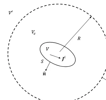
FIGURE 1.1
Intersection of the averaging function of a point charge with a surfaceS, as the charge crossesSwith velocityv: (a) at some timet=t1, and (b) att=t2> t1. The averaging function is represented by a sphere of radiusa.
magnetic moments of particles). The assumption of a sufficiently large averaging radius leads to
J(r, t) =ρ(r, t)v(r, t).
The total fluxI(t) of current through a surfaceS is given by
I(t) = Z
S
J(r, t)·nˆdS
where ˆnis the unit normal toS. Hence, using (1.5), we have
I(t) =X
i qid
dt(ri(t)·nˆ)
Z
S
f(r−ri(t))dS
if ˆnstays approximately constant over the extent of the averaging function andS is not in motion. We see that the integral effectively intersectsS with the averaging function surrounding each moving point charge (Figure 1.1). The time derivative ofri·nˆrepresents
the velocity at which the averaging function is “carried across” the surface.
Electric current takes a variety of forms, each described by the relationJ=ρv. Isolated charged particles (positive and negative) and charged insulated bodies moving through space compose convection currents. Negatively charged electrons moving through the positive background lattice within a conductor compose aconduction current. Empirical evidence suggests that conduction currents are also described by the relation J =σE known asOhm’s law. A third type of current, calledelectrolytic current, results from the flow of positive or negative ions through a fluid.
1.3.2
Impressed vs. secondary sources
In addition to the simple classification given above, we may classify currents asprimary
orsecondary, depending on the action that sets the charge in motion.