Vol. 44 (2001) 177–200
The information advantage in two-person bargaining
with incomplete information
Darryl A. Seale
a, Terry E. Daniel
b, Amnon Rapoport
c,∗aUniversity of Nevada Las Vegas, Las Vegas, Nevada, USA bUniversity of Alberta, Edmonton, Alberta., Canada cDepartment of Management and Policy, University of Arizona,
405 McClelland Hall, Tucson, AZ 85721-0108 USA
Received 12 October 1998; received in revised form 5 July 1999; accepted 8 July 1999
Abstract
The sealed-bidk-double auction is a mechanism used to structure bilateral bargaining under two-sided incomplete information. In the process of testing whether or not the observed bid and ask functions are in agreement with the Bayesian linear equilibrium solution under asymmetric information conditions, we find a strong information disparity effect. The trader favored by the information disparity, whether buyer or seller, receives a significantly larger share of the realized gains from trade than that predicted by the theory. A reinforcement-based learning model is formu-lated and tested. It accounts successfully for most of the variability in the round-to-round individual decisions. © 2001 Elsevier Science B.V. All rights reserved.
JEL classification:c72; c92
Keywords:Sealed-bidk-double auction; Bilateral bargaining; Information disparity; Reinforcement-based learning
1. Introduction
It is a commonly accepted truism that in bargaining situations ‘information is power’. Nearly all of the practical and academic literature on the topic highlights the advantage conveyed to the party knowing the most about the other’s position. In the bargaining situation considered in this paper, that of a buyer and a seller negotiating the sale price of a single item under two-sided uncertainty, information refers to how much each party knows about
∗Corresponding author. Tel.:+1-520-621-9325; fax:+1-520-621-4171.
E-mail address:[email protected] (A. Rapoport).
the reservation value of the other. The party that is most successful in narrowing down the uncertainty about the other’s value is usually best able to press for a favorable transaction price. The present paper reports on experiments that have uncovered a significant and robust information effect in bilateral bargaining.
In a seminal paper, Chatterjee and Samuelson (1983) constructed Bayesian Nash linear equilibrium strategies (LES) for the buyer and seller in the sealed-bidk-double auction mechanism and determined the profit that each person could expect from employing these strategies. In the course of a series of laboratory experiments, we have found general support for this model. However, with rare exceptions, we have also found that our sellers who were in a weak information position achieved significantly lower gains from trade than they could have obtained if they bid as LES suggests and our buyers, who were endowed with an information advantage, achieved significantly higher gains.
This paper proceeds as follows. We first describe the sealed-bidk-double auction mecha-nism and then present the LES for two bargaining situations examined in the present study. Our focus is on asymmetric two-person bargaining with incomplete information (Linhart et al., 1992) in which one of the traders has a distinct information advantage. In contrast to out previous studies (Daniel et al., 1998, hereafter DSR; and Rapoport et al., 1998, hereafter RDS), the information structure examined in the present paper favors the seller, not the buyer. We next present two new experiments that manipulate the amount of information that the seller possesses about the buyer’s reservation values. These experiments are mirror images of two previous experiments conducted by DSR in which the information advantage was conferred on the buyer. We exploit this feature of the design to measure the increase in profit that the trader-either buyer or seller-derives from the information advantage. Our results show that in the environment we examine property rights do not matter; rather, it is the infor-mation advantage that determines the change in profit from equilibrium play. They also show that the learning model proposed by DSR is equally applicable to account for the individual asks and bids in bargaining situations that favor the seller. The concluding section discusses the applicability of these results to less structured two-person bargaining situations.
2. The sealed-bidkkk-double auction mechanism
Consider a bilateral bargaining situation, where a seller has a single object that he may sell to the buyer if an acceptable price,p, is agreed upon. Assume thatVdenotes the buyer’s reservation value, the maximum price she is willing to pay for the item, andCdenotes the seller’s reservation value, the minimum price he is willing to accept for the same item. Both traders are assumed to be risk-neutral, expected utility maximizers, and their utility functions are normalized so that if no trade occurs then the utility of each is zero. If trade occurs, then the gains from trade for the seller and buyer arep−CandV−p, respectively. What each trader knows about the reservation value of the other is modeled in the follow-ing fashion. Each trader’s reservation value is a random variable whose value is contained in some interval. The reservation valuesCandVfor the seller and buyer, respectively, are ran-domly and independently drawn from the distributionsFandG. The two distributionsFand
Under the sealed-bidk-double auction mechanism, the seller submits an askcand simul-taneously the buyer submits a bidv. Ifk =1/2, as in the present study, trade occurs with no delay at the pricep=(v+c)/2 which is midway between the bid and ask, ifv≥c. If v < c, then negotiations end and no trade occurs.
The best known Bayesian Nash equilibrium solution for the sealed-bid mechanism with two-sided incomplete information is the LES of Chatterjee and Samuelson (1983). Leininger et al. (1989) have shown that there are many other Bayesian Nash equilibria for this mech-anism. However, Myerson and Satterthwaite (1983) proved that the LES maximizes the expected ex ante gains from trade achievable by any such mechanism. This provides justi-fication for its central role in the analysis of bilateral trading.
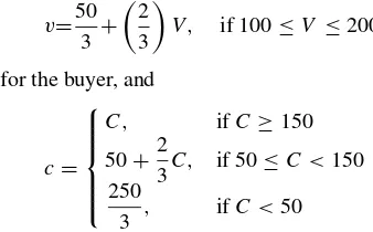
A strategy for a trader is a real-valued function, called thebid functionfor the buyer andask functionfor the seller, defined on the support of the distribution of this trader’s reservation value. It specifies an ask/bid for each reservation value. WhenFandGare both uniformly distributed over the interval [0, 100], the LES strategies are
ν=
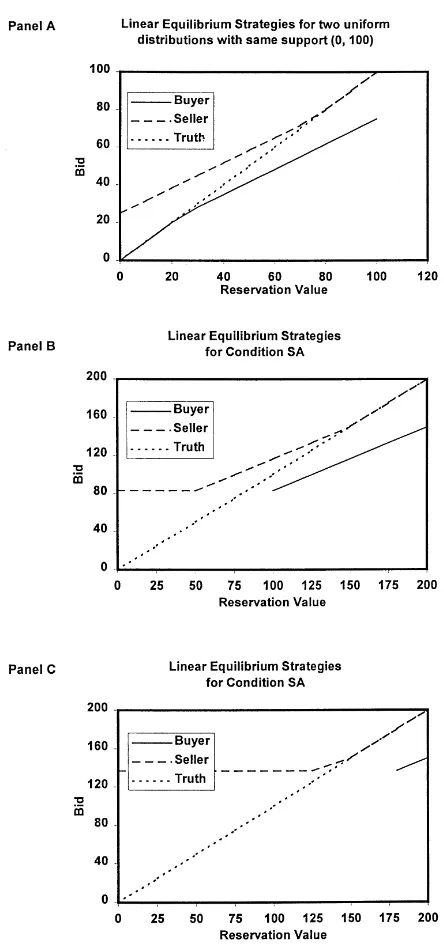
for the seller. These two equilibrium strategies are portrayed graphically in the top panel of Fig. 1. Both functions are piecewise linear and make only modest departures from the ‘truth telling’ line, which corresponds to a trader fully revealing his or her reservation value.
For the two experimental conditions reported on in this paper, an information asymmetry has been created which results in more distinct LES functions. In the first condition, called seller’s advantage (SA),F is uniformly distributed over the interval [0, 200], and Gis uniformly distributed over the interval [100, 200]. This represents a bargaining situation where the seller knows that the buyer’s best alternative for the object is equally likely to be any value between 100 and 200 (in monetary units). On the other hand, the buyer is less certain as to the seller’s value; it can be anywhere between 0 and 200. The LES strategies for condition SA are given by
In our second condition, the seller has a considerably larger advantage (SLA).Fis now uniformly distributed over the interval [0, 200], whereasGis uniformly distributed over the considerably narrower interval [180, 200]. In condition SLA, the seller has little doubt as to the value placed by the buyer on the item being traded. The pair of LES is given by
v=50
for the seller. These two functions are displayed in the bottom panel of Fig. 1. Contrast the distinct departures from the truth-telling line in the bottom panel with the nearly linear function in the top panel. The seller never asks less than 136.67 for any item, even one that he values at 0.
2.1. Previous experimental research
Following earlier studies by Radner and Schotter (1989), Schotter (1990), and Rapoport and Fuller (1995), in which the focus was on testing the model of Chatterjee and Samuel-son and on compariSamuel-sons between the LES and a model postulating truth-telling, DSR and RDS shifted the focus to information structures that favor the buyer. They did so by in-cluding the support of the seller’s prior distributionFin the support of the buyer’s prior distributionG. Their intention was to provide an environment in which LES behavior was distinctly different from truth telling. An unexpected finding of this study was that, rela-tive to the potential payoffs achievable under LES, the seller’s performance was distinctly worse than the buyer’s. Most of the buyers used bidding strategies that generally con-formed to the LES but with experience bid even more aggressively than predicted by the LES. On the other hand, the sellers tended to bid between the LES and truth telling levels, thereby achieving profits much lower than those attainable if both parties bid in accordance with LES.
While these studies have answered many questions regarding the strategic behavior of traders, they have also raised an important new one. What are the primary factors governing the realized gain from trade attained by each party? Radner and Schotter found that sellers more closely approximated the behavior posited by the LES than did the buyers, who tended not to shave their bids by amounts great enough to satisfy the LES prediction. Consequently, the sellers earned slightly more than they would expect if both traders played either truthfully or according to the LES. DSR, and subsequently RDS, reported the opposite results and hypothesized that this difference is attributable to the disparity in information between the seller and buyer that was introduced into their experiments. Radner and Schotter used prior distributions of reservation values with the same support for both traders. As a result, an explanation of their results must rest on other factors such as the possible perception on the part of both traders that the seller, endowed with the property rights, has intrinsic power.
To provide a more comprehensive test of the DSR hypothesis, one must also include information conditions favoring the seller. The present study compares the results of the previous two experiments by DSR to those of two new experimental conditions in which the information disparity favors the seller. Condition SA reverses the advantage provided to the buyer in Experiment 1 of DSR. The seller’s reservation value is drawn from a wider uniform distribution [0, 200] than is the buyer’s value [100, 200]. Likewise, con-dition SLA reverses the roles of buyer and seller in Experiment 2 of DSR. It provides an even stronger information advantage to the seller by restricting the buyer’s values to the interval [180, 200]. Our results show that these changes in the information provided to each trader have a profound effect on the profits they realize. Combined with the re-sults from the two previous studies, they present a powerful information effect in bilateral bargaining.
What would happen in the experiment of DSR or in the present experiment in which the information disparity is reversed if the traders in the weak position were to play more aggressively — more in accordance with LES? In a third experiment that we conducted, called condition BAC, the buyer’s reservation values are drawn from a uniform distribution on [0, 200] and the seller’s from a uniform distribution defined on [0, 100] as in Experiment 1 of DSR (in fact, the same sequence of values is used). Significantly, however, and unknown to the buyers (who were only told that they would be randomly matched with a seller on each round), the sellers areprogrammedto respond with LES asks on every trial of the experiment. Condition BAC is introduced to determine whether the buyer’s bids will be moderated when the seller is no longer willing to be ‘pushed down’.
3. Method
3.1. Subjects
Fifty undergraduate and graduate students from the universities of Arizona and Alberta participated as subjects in the three new experimental conditions reported in the present paper (SA, SLA, and BAC). In total, 130 subjects participated over the course of this study and the related ones of DSR and RDS. The subjects were recruited by advertisements placed in the university student daily newspapers promising monetary reward contingent on performance in a group decision making experiment. Both male and female students responded in nearly equal proportions. The mean payoff per subject was approximately $16.00. In addition, all the subjects received a fixed show-up fee of $5.00.
3.2. Experimental procedure
Each experiment lasted approximately 90 min with the first 20 min consisting of orienta-tion and instrucorienta-tions. For condiorienta-tions SA and SLA, 20 subjects participated simultaneously in a single session conducted in a laboratory containing 20 networked PCs separated by an aisle into two groups of 10. The twenty computer terminals were well separated from one another preventing communication between the subjects. Upon entering the laboratory, the subjects drew a token that determined their role in the experiment (i.e. seller or buyer). Buyers were seated in one section of the room and sellers in the other. In the third condition (BAC), the 10 buyers were matched with sellers in a separate room which, unknown to the buyers, were simply computer terminals programmed to respond with LES asks.
Each experiment started with instructions (a copy is available at http://cob.nevada.edu/ scale-www/barginst.htm) on the use of the individual terminals and the structure of the sealed-bid mechanism. The instructions were presented in writing as well as displayed on the computer monitor. The subjects were explicitly instructed that their bargaining partners were randomly varied from trial to trial. All 50 rounds were structured in exactly the same way. At the beginning of each round each seller and each buyer privately received a reservation value randomly drawn with equal probability from their respective distributions. To allow between-subjects comparisons, each trader received a different permutation of the same 50 reservation values.
Bargaining continued with buyer (seller) being prompted to state her bid (his ask) for the round. The computer required the subjects to confirm their responses and warned them if they might lead to a loss (i.e. ifct < Ct orvt > Vt). Prior to entering their responses, the subjects could review their previous responses and outcomes by calling up a separate screen. After all 20 subjects responded, the central computer determined for each pair separately whether a deal was struck, and calculated the payoff for each dyad member (eitherV −p or 0 for the buyer, and eitherp−Cor 0 for the seller). Subjects were then informed of their decision, their opponent’s decision, and if an agreement had been reached, the pricepand the gain for the round. Subjects proceeded at their own pace.
4. Results
This section provides graphical displays and statistical summaries of the results of the present study as well as compares these results with those of DSR. We begin with an analysis of the impact of information disparity on the decisions and profit of our subjects. Later in the paper we report the results of testing the learning model.
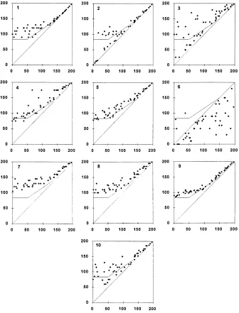
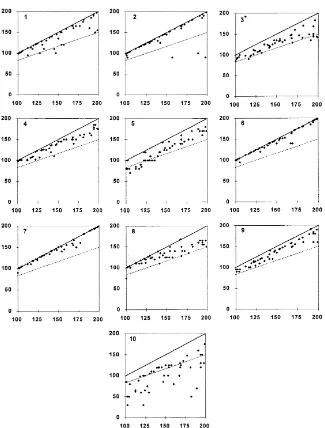
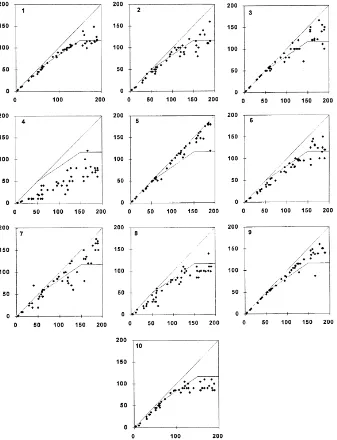
Condition SA: Fig. 2 displays the 50 asks (all the individual data points) plotted against the 50 reservation values for each of the 10 sellers in condition SA. Superimposed on the scatter plot is the piecewise LES Eq. (1). On the average, the individual plots show reasonable support for the piecewise linear prediction of the LES. Seven sellers (1, 4, 5, 7, 8, 9 and 10) followed the general pattern suggested by the LES, although many (for example, seller 7) bid more aggressively (higher asks) than the theory predicts. This tendency is the central focus of this paper and will be analyzed in detail below. sellers 2 and 3 exhibited LES characteristics in their bidding but also some inclination towards fully revealing their reservation values (‘truth-telling’). Seller 6 was the only subject of all of those who have been involved in our experiments over a 3-year period who clearly did not understand the task. In the interest of completeness his, results are included but appear spurious.
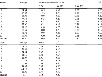
For each seller, we estimated a piecewise linear (spline function) to fit the data in Fig. 2. The top panel of Table 1 summarizes the results for the 10 sellers: it presents the intercept,
Table 1
Linear regression results for sellers and buyers in condition SA
Buyer Intercept Slopes by reservation value R2
Fig. 2. Bids vs. reservation values for individual sellers in condition SA.
three slopes for the ranges of reservation values 0–50, 51–150, and 151–200, and theR2
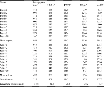
Fig. 3. Bids vs. reservation values for individual buyers in condition SA.
The LES slopes for the ranges 0–50, 51–150, and 151–200 are 0, 0.67, and 1.0, respec-tively. Except for seller 6, and the conservative asks of seller 2 in the 0–50 range, the LES appears to be a good approximation to the observed bid functions. The medians of the three slopes (below the top panel) clearly show the expected trend from strategic play for low reservation values to truth-telling for high reservation values.
full revelation of the reservation values. Four buyers (1, 2, 6, and 7) almost always placed bids very close to their reservation values. Five other buyers (3, 4, 5, 8 and 9) bid below their reservation prices but seldom as low as the LES values. Only buyer 10 consistently bid at or below the LES level and, as we shall see below, no buyer made as much money as she did.
The regression results for the buyers, presented in the lower panel of Table 1, tell the same story. There is as much support for the truth-telling model (slope=1, intercept=0) as there is for the LES model (slope=0.67, intercept=16.7).
Combining the results of the sellers and the buyers, we observe a general tendency of aggressive bidding by the sellers and conservative bidding by the buyers. The net impact of these observed tendencies on realized profits is summarized in Table 2. The left-hand column labeled A–A shows the actual payoffs (in a fictitious currency called ‘francs’ that
Table 2
Payoffs by actual and hypothetical strategies in condition SA
Trader Strategy pairs
A–Aa LE–Leb TT–TTc LE–Ad A–LEe
Buyer 1 710 985 1220 779 841
Buyer 2 995 1478 1696 1246 929
Buyer 3 1112 1218 1411 1235 1074
Buyer 4 1041 1245 1561 915 1231
Buyer 5 1006 1333 1544 1045 1223
Buyer 6 977 1237 1477 1192 900
Buyer 7 725 1164 1317 966 864
Buyer 8 894 1153 1363 898 1063
Buyer 9 978 1351 1474 1046 1154
Buyer 10 1142 1356 1563 1234 1203
Mean buyers 958 1252 1462 1056 1048
Seller 1 1919 1458 1505 1202 1761
Seller 2 1453 1310 1405 927 1667
Seller 3 1403 1394 1568 1004 1701
Seller 4 1721 1405 1457 1235 1806
Seller 5 1716 1328 1396 1026 1672
Seller 6 381 1408 1500 −99 1733
Seller 7 1571 1421 1556 567 1790
Seller 8 1477 1253 1323 977 1517
Seller 9 1855 1442 1548 1251 1821
Seller 10 1474 1245 1368 845 1583
Mean sellers 1497 1366 1462 894 1705
Overall mean 1227 1309 1462 975 1377
Percentage of deals made 55.8 51.8 75.8 38.2 63.4
aA–A: both traders play actual decisions as in experiment. bLE–LE: both traders play LES strategies.
were later converted into US dollars) for each trader. The percentage of rounds that resulted in trade (55.8 percent) is shown at the bottom of the column. The column labeled LE–LE shows the payoff that would have accrued (given the actual reservation values received in the experiment) if all the subjects had played the LES for the entire duration of the experiment. The next column labeled TT–TT shows the payoffs that would have resulted if all the traders truthfully stated their reservation values (thereby maximizing efficiency). The column labeled LE–A shows the payoffs that would have resulted if the buyers had played their LES strategies and the seller their actual strategies. In the right-hand column labeled A–LE the roles of buyer and seller are interchanged.
Column A–A shows that, on the average, the sellers earned 56 percent more than the buyers. In comparison, were both to play their LES, the sellers’ advantage would have declined to only nine percent. Comparison of columns 1 and 2 shows that the main source of this difference is the poor outcomes achieved by the buyers. Sellers gained slightly more than expected relative to the LES, but buyers gained considerably less (23 percent). Individually, these results hold for all 20 subjects with the exception of seller 6. The sealed-bid mechanism performed rather well; deals were struck in 55.8 percent of the rounds compared to 51.8 percent associated with LES play. Table 2 further shows that despite this relatively high percentage of trades made, more than six percent of the potential total profit achievable in the experiment under LES was left on the table.
Condition SLA: When the information disparity favoring the sellers is increased, the results are similar to those of condition SA with the payoff disparities magnified.
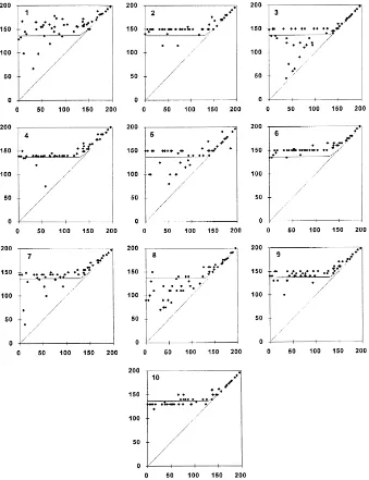
Fig. 4 displays the 50 asks plotted against the 50 reservation values for each seller sep-arately. The piecewise LES functions (Fig. 1) are superimposed on each scatter plot. The support for the LES prediction is as good as before. For six sellers (2, 4, 6, 7, 9, and, in particular, 10), the correspondence is remarkable. Most sellers made more aggressive asks than the LES whereas others deviated in the direction of truth-telling (sellers 3 and 8).
The bids of the 10 buyers (not displayed here) are similar to those reported in Fig. 3 for condition SA. Nearly all bids fall somewhere between the LES and the reservation values showing as much support for truth-telling as for strategic play. Only buyer 6 placed her bids at or below the LES level.
As in condition SA, we have a combination of most sellers in condition SLA bidding more aggressively than the LES and nearly all buyers bidding less aggressively. Using the same format as Tables 2 and 3 presents a summary of the payoffs that did or would have accrued to each trader. Again, we see a pronounced information effect. Column 1 of Table 3 shows that, on the average, the sellers in condition SLA earned 96 percent more than the buyers. In comparison, with both parties playing their LES, the sellers’ advantage would have been reduced to 41 percent. Comparison of columns 1 and 2 of Table 3 shows that, on the average, the sellers gained 11 percent more than expected relative to the LES whereas the buyers lost 20 percent. Individually, all buyers lost relative to the LES (compare columns A–A and LE–LE), and all but one of the 10 sellers gained. Table 3 further shows that deals were struck in 75 percent of all rounds compared to the 70.6 percent predicted by the LES.
Fig. 4. Bids vs. reservation values for individual sellers in condition SLA.
results of condition BAC, which replicates Experiment 1 of DSR in which the buyers had the information advantage.
Table 3
Payoffs by actual and hypothetical strategies in condition SLA
Trader Strategy pairs
A–A LE–LE TT–TT LE–A A–LE
Buyer 1 1372 1595 2117 978 1545
Buyer 2 1469 1725 2472 1036 1606
Buyer 3 1311 1692 2154 670 1409
Buyer 4 1492 1901 2462 965 1715
Buyer 5 1451 1767 2362 992 1492
Buyer 6 1110 1842 2374 841 1489
Buyer 7 1512 1798 2189 1123 1651
Buyer 8 1294 1616 2182 906 1349
Buyer 9 1673 1898 2326 1134 1665
Buyer 10 1440 1807 2422 851 1562
Mean buyers 1412 1764 2306 950 1548
Seller 1 2452 2497 2308 989 2849
Seller 2 2982 2511 2325 265 2891
Seller 3 2702 2503 2312 1236 2890
Seller 4 2726 2471 2261 1745 2635
Seller 5 2892 2505 2312 861 2881
Seller 6 2833 2510 2312 511 2793
Seller 7 2898 2512 2329 1570 2984
Seller 8 2551 2494 2296 1894 2910
Seller 9 2899 2494 2295 1476 2938
Seller 10 2853 2497 2310 2194 2871
Mean sellers 2778 2499 2306 1274 2864
Overall mean 2095 2132 2306 1112 2206
Percentage of deals made 75.0 70.6 96.4 33.4 81.6
reservation values as in the DSR study. The only difference was that the programmed sellers (unknown to the buyers) always bid their LES values.
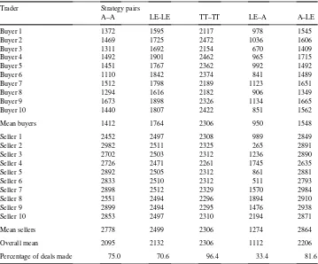
Fig. 5. Bids vs. reservation values for individual buyers in Experiment 1 of DSR.
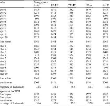
Table 4
Payoffs by actual and hypothetical strategies in condition BAC
Trader Strategy pairs
A–A LE–LE TT–TT LE–A A–LE
Buyer 1 1483 1549 1582 1549 1483
Buyer 2 1231 1412 1546 1412 1231
Buyer 3 1099 1463 1543 1463 1099
Buyer 4 698 1491 1624 1491 698
Buyer 5 1052 1409 1569 1410 1052
Buyer 6 1392 1542 1604 1542 1392
Buyer 7 1118 1416 1543 1416 1118
Buyer 8 1148 1426 1553 1426 1148
Buyer 9 1176 1474 1535 1474 1175
Buyer 10 1223 1454 1564 1454 1223
Mean buyers 1162 1464 1566 1464 1162
Seller 1 1486 1481 1582 1481 1485
Seller 2 1147 1234 1546 1234 1146
Seller 3 1405 1319 1543 1319 1405
Seller 4 415 1389 1624 1389 415
Seller 5 1744 1309 1569 1308 1745
Seller 6 1382 1545 1604 1545 1381
Seller 7 1337 1270 1543 1270 1338
Seller 8 1000 1345 1553 1345 999
Seller 9 1550 1388 1535 1388 1551
Seller 10 982 1395 1564 1395 982
Mean sellers 1245 1368 1566 1368 1245
Overall mean 1203 1416 1566 1416 1203
Percentage of deals made 42.6 52.4 76.4 52.4 42.6
Experiment 1 of DSR
Mean buyers 1457 1439 1536 1577 1182
Mean sellers 1028 1315 1536 1125 1112
Overall mean 1242 1377 1536 1125 1147
Percentage of deals made 51.6 52.6 77.0 57.8 40.8
improve those of the sellers and greatly reduce those of the buyers. This analysis, of course, ignores any changes the buyers might make during the experiment if sellers were to bid in this fashion. Table 4 shows that actual buyers, in the face of such aggressive bidding by the sellers, would adaptively retreat during the experiment and the sellers would do even better. In fact, the mean asks of the nine sellers excluding seller 4 (who faced the inflexible buyer 4) is nearly as high as the expected LES values. Clearly there is a lesson to be learned here; this topic is explored further in the concluding section of the paper.
5. A reinforcement-based adaptive learning model
the focus of the model is on individual not aggregate behavior, and the goal is to account for the round-to-round changes in the decisions of both buyer and seller. The model makes minimal demands on the rationality and reasoning ability of the traders. It assumes that the trader-seller or buyer-remembers what worked well (poorly) for him in the last round of bargaining, and then does it more (less) frequently in the future. The model strives at parsimony. We subscribe to the approach (e.g. Cooper and Feltovitch, 1996) that more cognitively demanding models should be employed only after the simpler ones are proven incapable of accounting for the data.
The learning model in DSR maintains consistency with basic principles of learning be-havior, particularly with the effects of reinforcement, as observed and documented in the vast psychological literature on animal and human learning. It embodies the ‘Law of Effect’ of Thorndike (1898), the ‘Power Law of Practice’ due to Blackburn (1936), the evidence about the generalization of stimuli reported by many psychologists, and the role of reference points in determining if outcomes are perceived as positive or negative gains (Kahneman and Tversky, 1979). Predecessors include the learning direction theory (Selten and Buchta, 1994) and the reinforcement-based learning model proposed and tested by Roth and Erev (1995). As with the Roth/Erev model, the DSR model makes no cognitively demanding assumptions involving probability distributions over the opponent’s actions or Bayesian updating of beliefs. It differs from the Roth/Erev model by replacing their probabilistic re-sponse mechanism with a deterministic, and consequently more easily refutable mechanism; by considering continuous rather than finite strategy sets with a small number of elements; by using a different approach to modeling stimulus generalization; and by postulating a smaller number of free parameters.
5.1. The buyer’s model
The buyer’s strategy is assumed to be a function specifying how much below her reser-vation value she should bid for the item being transferred. On any trialt, the amount that the buyer bids,vt, relative to her reservation value on that trial,Vt, is assumed to be described by the following function:
Eq. (4) defines an exponential function with the constraint that the bid cannot exceed the buyer’s reservation price. The free parameterbt determines the shape of the exponential function at roundt and hence the degree to which the buyer shades her bid below her reservation value on that trial. Smaller values ofbt represent more aggressive bidding. Thus, the buyer’s strategy space is represented by a one-parameter family of exponential functions. Although this family of functions does not include the piecewise linear LES function, a close approximation can be achieved, with the proper choice of parameters.
tendency to bid below the reservation price is reinforced and the buyer shades her bid more next time) in proportion to the profit realized, namely,Vt−pt, wherept =(vt +ct)/2 is the price of the transaction on roundt. Thus, following a successful trade on trialt−1,
bt =bt−1(1−w+b,t(Vt−pt)), (5)
wherew+b,t =(1−db)w+b,t−1is an impact factor that incorporates the relative effect of a positive outcome, anddb(0 < db≤ 1) is a discount factor that depreciates the impact of the outcome as time evolves.
If no trade takes place because the buyer bids too low on trialt(vt < ct), thenbt+1is adjusted upwards in proportion to the profit that the buyer could have made had she correctly forecast the seller’s asking price. However, if no trade occurs because the seller’s asking price exceeds the buyer’s reservation price (and hence no rational bid by the buyer would have resulted in a trade), then the buyer has no reason to change her bidding policy and
bt+1remains unchanged. The following equation captures both of these effects:
bt =bt−1·max(1,1+wb−,t(Vt−ct)), (6) wherew−b,t=(1−db)w−b,t−1is an impact parameter for profits lost due to greedy bidding, anddbis as defined above.
5.2. The seller’s model
The sellers model is identical to the buyer’s model with the only change being in the labeling of the parameters. Corresponding to a reservation value on roundtofCt ,the seller is assumed to place an ask,ct, determined by
ct =max
is the upper limit of the interval of the seller’s reservation values (S+
=200 in both conditions SA and SLA). Successful or unsuccessful transactions on roundt−1 are assumed to change the value of the parameterstand, consequently, the entire offer function, as follows:
st =st−1(1−ws+,t(pt−Ct)), ifvt ≥ct (8) and
st =st−1·max(1,1+w−s,t(vt−Ct)), ifvt < ct wherew+
to place the responsibility for the loss of transaction on the buyer, and consequently leaves his ask function unaltered.
In summary, the buyer’s bids are accounted for by four parameters:bt — the single parameter of the exponential bid function,wt+andw−t — the two impact parameters for successful and unsuccessful trades, anddb — a parameter discounting the effects ofw+ andw−. The seller’s asks are described by the same reinforcement-based learning model.
6. Dynamic analysis
In an attempt to account for the round-to-round decisions of the sellers and buyers in our experiments, the DSR learning model was estimated and tested on theindividual(rather than aggregate) level. For each of the twenty sellers and buyers in conditions SA and SLA, the four parameters of the learning model were estimated separately so as to best replicate the individual decisions of that trader. The estimation was conducted in the following manner. For each trader separately, the data were divided into two blocks of 30 and 20 trials respectively. A quasi-Newton search procedure was used to find the set of values of the four parameters that minimize the sum of squared errors between observed and predicted decisions over the first 30 trials. As is generally the case with such non-linear minimization procedures (Hamilton, 1992), there is no guarantee of achieving absolute minimum; the error function may have several local minima relative to the parameters of both the buyer’s and seller’s models. Using the best set of parameters thus found, the model was tested on the second block of 20 trials.
Table 5 presents the estimated parameter values for all the 20 traders in condition SA. The top section of the table displays the results for the buyers and the lower part for the sellers. In each case, the estimated values are based on the first 30 rounds of play. The performance of the fitted model over the last 20 rounds is shown in the two right-hand columns of the table. Two statistics are used to measure goodness of fit: R2, which measures the linear relationship between observed and predicted decisions, and the root mean squared error (RMSE) between observed and predicted decisions.
Beginning with the sellers in condition SA, the lower panel of Table 5 shows that the learning model describes the individual asks very well for all except seller 6 (our ‘irrational’ subject). Omitting seller 6, the medianR2is 0.94. The learning model is equally successful in accounting for the buyers’ bids. The top panel of Table 5 shows that the model provides an excellent description of the last 20 offers in nearly all cases; theR2values are above 0.90 for buyers 1, 2, 4, 5, 6, 7, and 9.
Consider next the estimated parameter values in Table 5. For the sellers, the discount values,db,vary between 0.00 and 0.21 with a mean of 0.05, and for the buyers they vary between 0.00 and 0.15 with a mean of 0.04. The difference in mean rate of learning between the buyers and sellers is not significant (t10 <1). Hence, for both buyers and sellers, the impact of profits and lost profits on future bids declines at approximately the same rate, namely, about five percent per period.
Table 5
Individual parameters and fit of learning model for condition SA
Buyer Parameters Trials 1–30 Trials 31–50
db w+ w− b0 R2 RMSE R2 RMSE
1 0.01 0.0001 0.0500 400 0.89 10.76 0.99 6.80
2 0.01 0.0001 0.0500 1000 0.39 23.90 1.00 6.29
3 0.06 0.0054 0.0500 700 0.93 7.05 0.88 11.08
4 0.02 0.0020 0.0500 700 0.92 7.15 0.96 5.53
5 0.09 0.0062 0.0000 2230 0.94 9.15 0.98 11.15
6 0.00 0.0000 0.0500 800 0.97 5.88 1.00 6.75
7 0.00 0.0000 0.0400 800 0.98 6.42 1.00 5.77
8 0.02 0.0016 0.0106 700 0.89 8.87 0.86 8.56
9 0.02 0.0016 0.0150 1000 0.98 7.75 0.94 6.46
10 0.15 0.0091 0.0000 1000 0.47 25.61 0.81 25.84
Mean 0.04 0.0026 0.0316 933 0.84 11.25 0.94 9.42
Seller ds w+ w− s0 R2 RMSE R RMSE
1 0.10 0.0053 0.0000 400 0.94 8.81 0.91 8.53
2 0.00 0.0026 0.0232 788 0.97 16.17 0.81 17.72
3 0.04 0.0002 0.0010 500 0.91 16.84 0.70 49.31
4 0.02 0.0050 0.0500 284 0.89 13.39 0.87 15.22
5 0.04 0.0045 0.0500 250 0.94 7.74 0.98 7.32
6 0.00 0.0000 0.0000 1000 0.38 57.75 0.52 45.21
7 0.05 0.0070 0.0100 175 0.81 12.09 0.94 6.51
8 0.21 0.0079 0.0000 287 0.94 9.23 0.94 9.49
9 0.01 0.0010 0.0200 180 0.97 6.48 0.94 7.17
10 0.05 0.0034 0.0232 200 0.85 12.25 0.94 17.00
Mean 0.05 0.0037 0.0177 406 0.86 16.08 0.86 18.35
reference points suggests stronger effects associated with losses than with gains.1 In terms of our learning model, the implication is thatw−> w+. Table 5 shows that this prediction holds for seven of nine sellers (omitting seller 6 again) and eight of the 10 buyers. The mean value ofw−is 0.0177 for the sellers whereas the meanw+is just 0.0037. This difference is significant (F =5.07,p≤0.037). For the buyers, the means are even more significantly different. The meanw−is 0.0316 compared to the meanw+ at 0.0026 (F =16.5,p ≤ 0.0007).
Tested in condition SLA, the learning model was clearly less successful for the buyers; the model accounts for only a small portion of the variation in their bids. Buyers’ reservation values were constrained to the narrow interval from 180 to 200, and most buyers appeared to change bids from trial to trial in a way that is largely independent of these values. For the sellers, the performance of the model was considerably better, but still not as good as for condition SA (medianR2is 0.84). The general observations regarding the impact of the two parametersw−andw+continue to hold under condition SLA.
6.1. Comparison of information advantage
Our study was designed to determine whether or not the information advantage conferred on buyers in the DSR experiment carried over to situations where sellers were given a corresponding advantage. As we observed in previous sections of the paper, the profit advantage buyers had in DSR translates into an equivalent advantage for sellers in conditions SA and SLA in the present study. One would then expect this symmetry to hold in the comparison of the two sets of experiments with respect to the estimated parameter values and the measures of goodness of fit of the learning model. Indeed, we find no significant differences between the two conditions. Table 6 shows that the learning model accounts equally well for the individual offers of the buyers in Experiment 1 of DSR as it did for the sellers in condition SA. TheR2 values are above 0.86 for all 10 buyers in Table 6. Discarding seller 6 in condition SA, the difference between the mean R2 values of the buyers in Experiment 1 of DSR and the sellers in condition SA is not significant (t17<1). Similarly, the mean RMSE scores do not differ significantly across the two sets of subjects. With the exception of buyer 2 in Table 6, the discount parameter,db, falls in a similar range for all buyers in Experiment 1 of DSR as it does for the sellers in condition SA, and the mean discount value is again about five percent. On the average, the meanw−value
Table 6
Individual parameters and fit of learning model for experiment 1 of DSR
Buyer Parameters Trials 1–30 Trials 31–50
db w+ w− b0 R2 RMSE R2 RMSE
1 0.04 0.0008 0.0063 250 0.91 13.45 0.95 17.98
2 0.30 0.0016 0.0500 173 0.82 14.36 0.92 9.37
3 0.02 0.0036 0.0294 170 0.94 10.00 0.94 8.10
4 0.03 0.0031 0.0100 600 0.89 15.23 0.93 9.29
5 0.00 0.0031 0.0651 400 0.85 16.57 0.94 10.58
6 0.11 0.0017 0.0299 170 0.94 11.57 0.95 9.60
7 0.02 0.0024 0.0209 115 0.91 9.37 0.96 7.51
8 0.06 0.0012 0.0001 275 0.89 16.64 0.88 9.82
9 0.00 0.0014 0.1000 800 0.89 23.19 0.86 27.74
10 0.03 0.0013 0.1000 500 0.90 22.55 0.95 16.31
Mean 0.06 0.0020 0.0412 345 0.89 15.29 0.93 12.63
Seller ds w+ w− s0 R2 RMSE R RMSE
1 0.06 0.0022 0.0052 500 0.83 9.66 0.93 10.05
2 0.10 0.0070 0.0200 400 0.89 7.49 0.76 15.45
3 0.00 0.0026 0.0265 200 0.67 15.03 0.92 14.38
4 0.05 0.0015 0.0138 400 0.37 25.10 0.71 18.37
5 0.12 0.0100 0.1000 500 0.46 27.92 0.44 26.07
6 0.11 0.0100 0.0000 1500 0.24 29.36 0.28 51.34
7 0.11 0.0059 0.0359 349 0.77 8.93 0.73 11.16
8 0.01 0.0002 0.0500 700 0.97 6.44 1.00 3.59
9 0.02 0.0008 0.0700 300 0.97 7.36 0.98 6.17
10 0.03 0.0010 0.0700 300 0.97 7.26 0.98 5.94
exceeds the meanw+by a factor of six for the sellers and 11 for the buyers. These results are in close agreement with the ones reported earlier in Table 5. We find no significant differences between the meanw−of the sellers in condition SA and the buyers in the DSR study. The same holds for the comparison of these two sets of traders with respect to the mean of the weight parameterw+. Statistical comparisons of the mean estimated values ofw−andw+between the buyers in condition SA and sellers in the DSR study also yield non-significant differences.
7. Discussion and conclusions
In a series of experiments originally designed to investigate the degree to which subjects in a sealed-bidk-double auction play according to the LES, a strong information effect has been observed. Initial results reported by DSR indicated that a buyer with an information advantage over a seller gained significantly higher profits from trade than suggested by the theory. The results of the present paper show that the effect is more general. Any trader in a sealed-bidk-double auction, buyer or seller, whose reservation values are drawn from a wider support than that of his trading partner, garners a larger share of the gains from trade than predicted by the LES. Correspondingly, the disadvantaged trader gains less than expected. Of prime interest are the results of a subsequent experiment (BAC) indicating that this advantage/disadvantage can be entirely erased if the trader in the inferior information position behaves more aggressively in accordance with the prescriptions of the theory.
Subsequent to the DSR study, it had been argued (including by several subjects in post experimental interrogations) that there was a good reason why sellers failed to turn the tide of initial aggressive bidding by the buyers. Each seller saw a randomly selected buyer, from a set of 10, on each trial and hence had no opportunity to ‘take a few losses’ and thereby establish a reputation as a tough bargainer for future trials. Buyers were influenced by the ‘field’ of sellers, and each individual seller had little impact. The RDS study put this argument to rest. When sellers faced the same buyer for a sequence of 50 trials, the information advantage persisted and was even marginally enhanced.
In contrast, the results of this paper illustrate that traders with an information disadvan-tage can greatly reduce or even overcome this disparity by bidding more aggressively. In condition BAC, sellers with the same information disadvantage as in Experiment 1 of DSR, but bidding strictly according to the LES function, were able to take all of the surplus profit away from buyers. All but one of the buyers in this experiment retreated to more conservative bidding in the face of higher asking prices by the sellers. As a result, sellers made nearly 25 percent more profit but to do so they had to accept more lost deals (particularly in the early rounds). Collectively, our experiments show that subjects seem unwilling to take these early losses to establish bargaining norms that will pay off later. The information structure is such that if an initial advantage (often more apparent than real) is conveyed to one party, then the other trader has great difficulty in overcoming these early misperceptions and attaining the profits the theory suggests he should attain. Condition BAC, however, illustrates that, with bidding discipline, the tables can be turned.
This is an important result for those who often bargain. In nearly all real bargaining circumstances, disparate information is present. If the results of these experiments are valid, it appears as if those parties who have less information underachieve relative to the information they do have. The question remains as to whether or not these results, obtained using a highly structured mechanism, apply to more common open-ended bargaining. We would argue that to a significant degree they do. One can view the back and forth sequence of bids and asks in traditional face-to-face bargaining as preamble to the ‘final positions’ that the traders take. The strategies of the traders are in essence these final positions-how high the buyer will go and how low a price the seller will accept. If both traders are immune to the dynamics and cheap talk of the preceding sequence of bids and asks, then the LES solution of Chatterjee and Samuelson remains relevant to the determination of the final position of each trader. The seller and buyer should not view their reservation values as the lowest and highest prices, respectively, that they will accept. If one accepts this congruence of the sealed-bidk-double auction and face-to-face bargaining, then one would expect that traders who know less about the reservation value of their trading partner than vice versa will realize gains from trade in face-to-face bargaining that are lower than they could be with more aggressive decisions.
Acknowledgements
References
Blackburn, J.M., 1936. Acquisition of skills: an analysis of learning curves. IHRB Report No. 73.
Chatterjee, K., Samuelson, W., 1983. Bargaining under incomplete information. Operations Research 31, 835–851. Cooper, D.J., Feltovitch, N., 1996. Selection of learning rules: theory and experimental evidence. University of
Pittsburgh, Department of Economics, Working Paper No. 305.
Daniel, T.E., Seale, D.A., Rapoport, A., 1998. Strategic play, strategic play and adaptive learning in the sealed bid bargaining mechanism. Journal of Mathematical Psychology 42, 133–166.
Hamilton, L.A., 1992. Regression Analysis with Graphics. Wadsworth, Belmont, CA.
Kahneman, D., Tversky, A., 1979. Prospect theory: an analysis of decision under risk. Econometrica 47, 263–291. Leininger, W., Linhart, P.B., Radner, R., 1989. Equilibria of the sealed-bid mechanism for bargaining with
incomplete information. Journal of Economic Theory 48, 63–106.
Linhart, P.B., Radner, R., Satterthwaite, M.A. (Eds.), 1992. Bargaining with Incomplete Information. Academic Press, San Diego.
Myerson, R.B., Satterthwaite, M.A., 1983. Efficient mechanisms for bilateral trading. Journal of Economic Theory 29, 265–281.
Radner, R., Schotter, A., 1989. The sealed-bid mechanism: an experimental study. Journal of Economic Theory 48, 179–220.
Rapoport, A., Daniel, T.E., Seale, D.A., 1998. Reinforcement-based adaptive learning in asymmetric two-person bargaining with incomplete information. Experimental Economics 1, 221–253.
Rapoport, A., Fuller, M., 1995. Bidding strategies in a bilateral monopoly with two-sided incomplete information. Journal of Mathematical Psychology 39, 179–196.
Roth, A.E., Erev, I., 1995. Learning in extensive-form games: experimental data, and simple dynamic models in the intermediate term. Games and Economic Behavior 8, 164–212.
Schotter, A., 1990. Bad and good news about the sealed-bid mechanism: some experimental results. American Economic Association Papers and Proceedings 80, 220–226.
Selten, R., Buchta, J., 1994. Experimental sealed bid first price auctions with directly observed bid functions. In: Budescu, D.V., Erev, I., Zwick, R. (Eds.), Human Behavior and Games: Essays in Honor of Amnon Rapoport. Erlbaum, Mahwah, NJ, pp. 79–102.