Heating technology and energy use:
a discrete
r
continuous choice approach to
Norwegian household energy demand
Kjell Vaage
UDepartment of Economics, Uni¨ersity of Bergen, Fosswinckelsg. 6, 5007 Bergen, Norway
Abstract
The aim of this paper is to describe the structure of the household’s energy demand as a discretercontinuous choice and, on this basis, establish an econometric model suitable for the data available in the Norwegian Energy Sur¨eys. The discrete appliance choice is
Ž
specified as a multinomial logit model, with a mixture of appliance attributes operating
. Ž .
costs and individual characteristics income, housing unit characteristics, etc. as explana-tory variables. In the next step the continuous choice of energy use is modelled conditional on the appliance choice. The energy prices turn out to be significant both when estimating the appliance choice and the conditional energy demand. The estimated price elasticity for energy exceeds minus unity. The paper discusses how this relatively strong price response should be interpreted in the context of other econometric analysis with no explicit appliance dependence. Finally, the significance of the many household characteristics at both stages of the model signals a high degree of heterogeneity within the households, which justifies the use of detailed micro-data in the modelling of the energy demand.Q2000 Elsevier Science
B.V. All rights reserved.
JEL classifications:C25; D12
Keywords:Residential energy demand; Discretercontinuous choice
1. Introduction
A salient feature of the demand for energy is its inherent dependence on indivisible household durables. Energy is not used directly, rather, it is used to
U
Tel.:q47-55-58-92-06; fax:q47-55-58-92-10.
Ž .
E-mail address:[email protected] K. Vaage .
0140-9883r00r$ - see front matterQ2000 Elsevier Science B.V. All rights reserved.
Ž .
power appliances that produce services such as heatingrcooling, cooking, lighting, etc. This has motivated the search for dynamic models in analysis based on time series data, since a household’s response to changes in, e.g. relative prices, is different in the short-run, when the demand is limited by the given stock of installations, than in the long-run, when the appliance has been optimally adapted to new conditions. Econometric analyses of residential energy demand based on aggregated time series data are numerous; Norwegian studies include Rødseth and
Ž . Ž . Ž .
Strøm 1976 , Bjerkholt and Rinde 1983 , Vaage 1995 .
Cross-sectional micro data for Norway are, however, available through three extensive surveys carried out by the Central Bureau of Statistics in 1980, 1983, and
Ž . Ž . Ž .
1989, which are documented in Hem 1983 , Ljones 1984 , Ljones et al. 1992 , respectively. Of course, cross-sectional data do not allow a true study of dynamics. They do, however, allow a focus on the relationship between energy demand and the stock of energy using appliances. This relationship is as follows.
The first decision involved in energy consumption is the choice of energy appliance. Then, conditional on this choice, the household decides how to utilise the given stock. Since these are related decisions, the two choices must be modelled jointly to avoid biased and inconsistent parameter estimates. The econo-metric analysis of the utilisation decision can be treated in a conventional manner in that the demand variable can be assumed to vary continuously with its explana-tory variables. The appliance choice, on the other hand, is a typical example of a discrete variable, since the households have to choose among a limited number of appliances. The primary aim of this paper is, accordingly, to describe the structure of the household’s energy demand as a discretercontinuous choice, and, on this basis, establish an econometric model suitable for the data available in the Energy Sur¨eys. Due to data limitations we are restricted to concentrate on the choice of heating technology.
A unifying theoretical exposition of the discretercontinuous choice approach is
Ž .
found in Hanemann 1984 . Based on the same approach Dubin and McFadden
Ž1984 , present an econometric analysis of residential electric appliance holdings in.
Ž .
the US, while Nesbakken and Strøm 1993 apply the 1990 Energy Survey in a discretercontinuous model for the energy demand in Norwegian households.
Ž .
Dagsvik et al. 1987 present an extension to a dynamic discretercontinuous choice model, and apply their model in an analysis of gas demand in the residential sector in western Europe.
In Section 2 we describe the structure of the discretercontinuous choice model, and show how the model can be represented in a form that allows econometric estimation. Section 3 presents the Energy Sur¨ey data, while Section 4 reports and discusses the results from the econometric analysis. Section 5 provides some concluding remarks.
2. The model
Ž .
main concern is the modelling of demand for different brands of a commodity, we adapt the same approach to the residential energy demand.
Hanemann formulates a model where both the discrete and the continuous consumer choices are derived from the same utility maximisation problem. Broadly speaking, this is a question of finding a random indirect utility function which, when the random component is specified, can be used to derive a model for the estimation of choice probabilities for different heating technologies. Conditional on the chosen technology, energy demand functions are derived by applying Roy’s identity to the same indirect utility function. This will now be demonstrated step-by-step.
Suppose x is a continuous vector measuring the consumption of N different energy sources in a given household. We start out with the following utility function:1
Ž . Ž .
usu x,b,z,s,« 1
where x is a vector of goods and zis a numeraire, bis a vector of characteristics of
x, s is a vector of characteristics of the individual, and « is a random component. The discrete choice is to decide whether or not xi is to be zero, while the continuous choice is to decide how much xi to use, given that xi)0 in the first step.
As in all other works referred to in this article we restrict our household to
2 Ž .
choose only one heating alternative. Hanemann 1984 does this by choosing utility functions that restrict the indifference curves to be linear or concave and thereby ensure corner solution.3
Ž
Suppose that a consumer decides to choose good i with corresponding
tech-.
nology . Given this choice we get the conditional utility function:
Ž . Ž .
uisui, xi,bi,z,s,« 2
that is maximised subject to p xi iqzFy and xi, zG0. We then define the conditional indirect utility function as:
Ž . w Ž . Ž . x Ž .
¨i pi,bi,s,« 'u xi i pi,bi,y,s,« ,bi,z pi,bi,y,s,« ,s,« 3 By Roy’s identity the continuous-choice demand for energy, conditional on the choice of technology i, can be derived as:
1
The household index is omitted for ease of exposition. 2
The majority of the households participating in theEnergy Sur¨eyhave installed heating technology that can combine or switch between electricityrsolid fuelroil. This must not be confused with multiple appliance choice; still the households are grouped according to single choices like electricity, oil, oilqelectricity, etc.
3
Ž .
To find econometric models for choice probability and energy use, we have to i describe the random component «i and specify how it enters the utility function
Ž .
and ii choose a specific form of the utility function’s non-random components. We start with the former part:
A household chooses appliance irconsumption of energy good xi if the utility from this alternative exceeds the utility from all other choice alternatives. If the
Ž .
indirect utility is decomposed into a non-random part, wisw pi i,bi,y,s , and a random part,«i, the choice probability, Pi, may be expressed as:
Ž .
PisPr w
iq«iGwjq«j, alli/j4
sPr«iy«j-wiywj, alli/j4
. 5 Assuming that «i is independent and identical type I extreme value distributed,Ž .4
the choice probability can be expressed by the multinomial logit model MNL :
wi
As for the randomness of the utility function, Hanemann 1984 assumes that it is introduced through the econometrician’s limited possibility of observing the household’s evaluation of the quality of the different goods. Instead of letting b, the characteristics of x, enter the utility function directly, the quality index ci is
Ž .
constructed as a function of K non-random properties of good i, bi k, and the random component «:5
It is now the quality index that enters the utility function. By assuming that the consumers maximise the product cixi and letting all N arguments be entered additively:
maximisation subject to the budget constraint will result in a corner solution.6 The
restriction of energy goods as perfect substitutes is thereby taken care of.
Given the choice of goodrtechnology i the conditional utility function, ui, will be given by:
U
Ž . Ž . Ž .
u xi i,ci,z,s sui cixi,z,s . 9
Ž .
Muellbauer 1976 has shown that this gives the following conditional demand and indirect utility functions: Hence, quality and quantity affect the consumer’s utility in identical ways; a doubling of quality, for example, will give the same increase in utility as a doubling in quantity. If this is carried over to the demand and indirect utility functions, we obtain that quality improvements are equally evaluated as price reductions; the consumers adapt, accordingly, to ‘quality per money’.
As noted earlier, alternative i is chosen if
UŽ . UŽ .
¨i pirci,y,s G¨j pjrcj,y,s .
In Hanemann’s setting income, y, and other individual characteristics, s, affect the indirect utility function, but not the choice probability.7 This implies that the
choice of alternative i depends entirely on pirci. Furthermore, in Hanemann’s formulation the discrete choice does not depend on the parameterisationof pirci.
Ž .
The choice probability may, therefore, be expressed in logarithmic form as:
4 Ž .
PisPr logpiylogciFlogpjylogcj, all i/j , 12
Ž .
and with Eq. 7 substituted for ci we get:
K K
Ž .
PisPr
½
«iqaiqÝ
gkbi kylogpiG«jqajqÝ
gkbjkylogpj5
13ks1 ks1
We will maintain Hanemann’s convenient representation of the prc ratio,8
i i
but in addition we wish to allow choice probabilities to be influenced by income
Ž .
and other individual characteristics. Hence, Eq. 13 is extended to:
6 Ž .
A formal treatment of this property is found in Deaton and Muellbauer 1980 . 7
In other words, it is assumed that individual characteristics have identical impact on each choice alternative.
8
M K
where thebsand the dsare the respective variable coefficients. If all non-random components are collected in:
From Eq. 6 we see that the choice probabilities can now be expressed as:
M
which is the multinomial logit model. Note that all the parameters are scaled bym, which is a measure of the dispersion of the extreme value distribution.9 Hence, the
larger the dispersion, the less the effect from the explanatory variables. In other words, if the ‘uncertainty parameter’ m is ‘large’, the observed non-random variables explain little, whereas random elements explain a lot.
Values of m should be positive a priori; firstly, because a price increase for alternative i, measured by y1rm, should lead to a lower probability of choosing that alternative. Secondly, and even more fundamentally, negative m implies a negative dispersion of the EV distribution, which makes no sense.
As will be demonstrated below, an estimate ofm is needed in the estimation of
Ž .
the continuous choice of energy use. From what is explained above we now see that through the specification of the price variable in the indirect utility function,m
becomes identifiable as the inverse of the estimated price parameter from the discrete choice model.
The next step is to derive a model for the continuous choice of utilisation of the
9 Ž .
appliance stock. This is done by applying Roy’s identity to the chosen indirect
Ž .10
utility function. The following function is suggested by Hanemann 1984 , but extended to include individual characteristics:
Via Roy’s identity and some simplification this yields:
y1 Žry1.wi Žry1.«i Ž .
xisupi e e 19
For convenience we apply the logarithmic transformation:
Ž . Ž . Ž .
logxisloguylogpiq ry1 wiq ry1 «i. 20
Ž . Ž .
«i in Eqs. 19 and 20 are the random components conditionalon the choice of
11 where 0.5772 is the Euler constant. The expected value of logxi is therefore:
N
The term mlog
Ý
e q0.5772 is referred to as the selection term, andjs1
measures the extent to which the energy expenditures are influenced by the choice of heating technology. The interaction between the probability structure in the discrete choice problem and the conditional demand structure takes place in this term. Obviously, if our assumption that appliance choice and appliance utilisation are related decisions is correct, omission of this variable will introduce bias in the energy demand model. The use of appliance dummies in the demand equation, as
10
Hanemann proposes several conditional indirect utility functions that are suitable for the deriva-tion of condideriva-tional demand funcderiva-tions. His criteria are that they must belong to a class of utility functions that have the desired properties of corner solution, etc., and that they must lead to tractable demand models.
is sometimes suggested, will not solve this problem. On the contrary; if there are components that influence both the energy demand and the appliance choice, the appliance dummies would become correlated with the error term in the demand equation, resulting in parameter estimates that would be both biased and inconsis-tent.
N
wjrm
m is identified in the estimation of the discrete choice. So is
Ý
e , which isjs1
the denominator in the multinomial logit expression. The variable in the curved bracket can, therefore, be calculated.
ry1 tells us how much the energy demand is influenced by the choice of
Ž .
heating alternatives. Hanemann 1984 notes that a necessary and sufficient condition for good xi to be essential with respect to the utility function is that
r-1, i.e. the estimate ofry1 should be negative a priori.
The energy prices in this model affect the technology choice through the operating costs. In addition, the price variable is allowed to have a direct effect on the conditional demand model. With the chosen parameterisation this direct price
12 Ž .
elasticity is assumed to be minus one, and Hanemann 1984 , therefore, suggests
Žthe log of the energy expenditure as dependent variable. We will, however, allow.
the price parameter to be estimated freely, and use the parameter’s closeness to minus one as a measure of the validity of the specification.
Income and other individual characteristics affect the energy demand through the selection term, but analogous to the price variable we want a specification where their potentially direct effect on the demand can be measured. This is achieved by making ua function of these variables. Let b,d1,....,dM be the impact on logxi from y,s1,...,sM, respectively. For convenience we choose logusa0q
Ž .
blogyqd s1 1q...qd sM M and the parameters b,d1,...,dM interpreted as direct conditional demand elasticities.
Accordingly, the estimating conditional demand equation becomes:
M
h is a conventional error term where zero mean and constant variance are
Ž .
assumed, so Eq. 23 may be estimated by OLS. Note that the parameters are equal for all energy alternatives. The N demand equations are, therefore, pooled and estimated simultaneously.
12
3. The data
Our data are based on an extensive survey on household energy consumption, organised by the Norwegian Central Bureau of Statistics in late spring 1980. A revision of the collected data together with an econometric analysis is documented
Ž .
in Hem 1983 . The survey covers 2289 households equally distributed throughout the country. It contains data on the following groups of variables:
3.1. Energy consumption and expenditures for each energy source
Electricity is the dominating energy source, representing approximately 65% of
Ž .
the households’ energy consumption. Other fuels are oil 25% and solid fuels
Žmostly burning wood. Ž10% . The data do not allow separation of consumption.
into heating vs. other purposes, but of a total consumption of 23.4 TWH in 1979,13
70]80% represented heating.
In addition to the respondents’ own answers, our data base contains information from the respective electricity utilities, giving the exact tariff type14 electricity
consumption and electricity expenditure for each interviewee.
3.2. Heating technology
The survey gives detailed information about existing installations. A distinct characteristic of the Norwegian household consumption is the high degree of combined heating technology. Of the households in the survey, 80% combine two or more fuels, while 11% are based solely on electricity, and only 9% on oil or wood.15
The interviewees are also asked to give some subjective characteristics on quality, plans regarding new installations, etc. Unfortunately, there are no objective measures of quality, nor any data on capital costs, data that are highly recom-mended when modelling the technology choice.
3.3. Building characteristics
Detailed information is available about age, type, floor area, number of rooms, ownership, etc. Obviously, these are important variables to include in the
conditio-13 Ž .
The fossil fuels are converted to KWH by converting factors reported in Hem 1983, p. 25 .
14 Ž .
Some 60% of the households belong to the group with increasing block price tariff ‘H3’ . It is well
Ž .
known, see, e.g. Taylor 1975 , that block pricing tariff might cause problems when calculating average
Ž
prices from expenditure data. However, we have reason to believe that this is a minor problem see
.
exogeneity tests in Vaage, 1995 , and continue as if electricity were available for each household at a
fixedprice. 15
nal demand model, but their potential influence on appliance choice will be tested for as well.
3.4. Inter¨iewees and household members
Data are available on geographic location, age, sex, occupation and education of the interviewed persons. The survey also reports on the number of household
Ž .
members, the number of children, gross household income before taxes , and the number of persons with income.
This provides us with a database quite suitable for modelling of the conditional energy demand, but with severe limitations with respect to a satisfying model of the appliance choice. The first problem is lack of data on appliance attributes, b .i k The
Ž . Ž .
quality index in Eq. 7 , therefore, has to be reduced tocisexp aiq«i. Hence,
Ž .
quality cleanness, comfort, controllability, flexibility, reliability, etc. is represented by appliance dummies,ai, plus the random component,«i.
The second problem is the insufficient price data for the different choice alternatives. The consumer choice of appliance purchase, replacement, and retire-ment is based on operating and capital costs of the alternative technologies. However, in the present survey only contemporaneous data on operating costs are available.16 Nevertheless, our view is that our cross-sectional data contains
impor-tant information: prices on all the different energy sources show large regional variation in our sample. As for oil prices, this is probably explained by the transportation costs. This also applies to wood; in addition, in rural areas it is common to have access to cheap burning wood through relatives and friends, a phenomenon that probably explains the huge price variation for this fuel. The Norwegian electricity pricing policy, which in 1980 was mainly based on each electricity utility’s historical costs, ensures a massive variation in electricity price as well. Hence, our data confirm large regional variation in relative operating costs for the different heating alternatives. The question is whether it makes sense to explain the dynamic phenomenon of choosing heating technology by contempora-neous relative prices. After all, we must expect that the majority of the households in our sample have based the choice of appliance on relative prices in a more or less distant past. Our point is that regional differences in relative prices are fairly stable over time, since they are explained by topography, historical costs, etc. Conditional on no migration, then, contemporaneous energy prices might actually be a good proxy for operating cost from the time in the past when the decision
Ž .
about appliance choice was taken. However, of course, other non-regional price movements, for example the oil price changes in the 1970s, weaken the quality of the current prices as a proxy for historical operating costs.
16 Ž .
Nesbakken and Strøm 1993 manage to complement the 1990 Energy Sur¨ey by collecting capital cost data. Armed with this improved database they present a discretercontinuous model in the spirit of
Ž .
In addition, to justify the use of contemporaneous operating costs to explain the appliance choice we have to assume static expectations. As noted by Dubin and
Ž .
McFadden 1984 , whose sample is also a cross-section, this assumption is at best only approximately true, and ideally should be tested against a more complete dynamic model, using panel data on consumer behaviour.
4. Results and discussion
The estimations are performed in two steps following a procedure suggested by
Ž .
Heckman 1979 . In the first step the discrete choice is estimated by maximum likelihood. The relationships between the observed choice i of the hth individualr
household, di h, and the explanatory variables are expressed with the following log likelihood function:
After substituting Eq. 17 for Pi h the log likelihood to be maximised becomes:
w rm
In the second step the conditional demand Eq. 23 is estimated by OLS, with the parameter estimated on the first step used to calculate the variable
represent-Ž .
ing the interaction between discrete and continuous choices the selection term .
4.1. The discrete choice
In the model the households face four different heating systems: electricity only
Ž .el , electricity in combination with solid and liquid fuels, respectivelyŽelrwood
. Ž .17
and elroil , and a combination of all three elrwoodroil . The percentage shares for the different alternatives are 5, 37, 23, and 35, respectively.
The energy price in the case of mixed heating technology is calculated as the average of the prices of the respective fuels. The prices of alternatives that are not
chosen are calculated as the average price for consumers using appliance j in the receptive county.18
Household characteristics included in the discrete choice model are gross
Ž . Ž .
household income Income, number of rooms in the building Rooms, a dummy
17
Households with solid or liquid fuels as the only heating source were too few to be included as separate groups.
18
Table 1
a
Ž .
Estimated coefficients, the discrete appliance choice alternatives :el,elrwood,elroil,elrwoodroil
Variable Choice Coefficient S.E. t-value
logPrice ] y0.4315 0.2182 y1.978
elrwood y0.0091 0.0024 y3.732
Income elroil y0.0021 0.0024 y0.882
elrwoodroil y0.0061 0.0024 y2.544
elrwood 0.1977 0.1185 1.668
Rooms elroil 0.1301 0.1213 1.073
elrwoodroil 0.3218 0.1188 2.708
elrwood y1.4649 0.3548 y4.129
Buildum elroil y1.9202 0.3877 y4.953
elrwoodroil y2.7743 0.4311 y6.436
elrwood y1.3930 0.3454 y4.034
Agedum elroil y1.6712 0.3688 y4.531
elrwoodroil y1.4912 0.3472 y4.295
elrwood y0.0420 0.3193 y0.132
Climdum elroil y0.5305 0.3374 y1.572
elrwoodroil y0.79950 0.3337 y2.396
elrwood 2.7128 0.4950 5.480
Appldum elroil 2.0288 0.5029 4.034
elrwoodroil 2.0730 0.4958 4.181
No. of observations 1307
Log-likelihood y1520.019
b
LR-test 161.866
a Ž .
The choice-specific coefficients are relative to the base categoryel electricity only . b
Likelihood ratio-test of H0: all coefficients but the constant terms equal zero.
Ž .
for building type Buildum, set to one for households living in blocks and zero for those living in detachedrundetached houses, a dummy for age of the building
ŽAgedum., set to one if built after 1975 and zero otherwise, and a dummy for warm
Ž .
climate Climdum, set to one for households in the five counties with highest average temperature and zero otherwise.19
To be able to identify the choice specific parameters, one of the alternatives has to be used as the base category; we have chosen the el-parameters to equal zero.
Ž .
Results from the estimation of the model in Eq. 17 are reported in Table 1. From the negative estimate of the price coefficient it follows, as expected a priori, that the model predicts lower probability for xi as the price of this alternative increases. Furthermore, the negative estimate implies that the disper-sion parameterm is positive, which is necessary for the model to make sense.
As for the estimated income coefficients, high household income appears to increase the probability of choosing electricity as the only heating device.
Combi-19
Continuous data on age of building and average outdoor temperature are not available in the
Ž .
nations with solid fuels wood are particularly unpopular among high-income households.
Both the type and the age of the building have significant impacts on the appliance choice. The estimates imply that households living in blocks choose electric heating more often than other households do; especially the combination
elrwoodroil is relatively infrequent in block apartments. Furthermore, heating technology based only on electricity appears to be more frequent in new buildings. Note that ‘new’ is defined as built in 1975 or later, which is the year after the first oil crisis. Not surprisingly, the appliance combination that includes oil has a particularly low probability of being chosen.
The number of rooms in the building and our measure of climate conditions do not influence the appliance choice in a significant way, except for the probability of choosing the elrwoodroil alternative. This alternative’s choice probability in-creases with the number of rooms, and dein-creases if the household is located in a relatively warm region.
Included in the discrete choice equation are also dummy variables for each of
Ž .
the respective alternatives named Appldumin Table 1 . The dummies should be interpreted as measuring unexplained attributes, i.e. attributes that influence the choice in question, but which are not accounted for by the explanatory variables. In Hanemann’s model these attributes are related to quality aspects, but also other properties may be accounted for by the dummy variables. It turns out that their coefficients are highly significantly different from zero. Nevertheless, the hypothe-sis that the constant terms represent all the explanatory power in the estimating equation is strongly rejected by the Likelihood Ratio test reported at the bottom of Table 1.
4.2. The continuous choice
Explanatory variables20 in the conditional energy demand equation are the
Ž . Ž . Ž .
selection term Select , energy price logPrice, income logIncome, and the household characteristics from the discrete choice equation: number of rooms
ŽlogRooms., type of building ŽBuildum., age of building ŽAgedum., and climate
ŽClimdum.. Hence, the energy price and the listed household characteristics are allowed to influence the energy demand directly, measured by their respective parameter estimates, and indirectly through their effect on the selection term.
Ž .
Finally, the potential direct impact from some additional household
characteris-Ž .
tics is tested for. These are the inside net floor area logFloor , the number of
Ž .
persons in the household logPerson, a dummy for whether there are small
Ž .
children in the household Childum, set to one if children and zero otherwise, and
Ž .
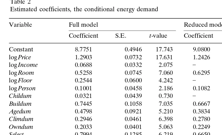
an ownership dummy Owndum, set to one if the apartment is rented and zero otherwise. Table 2 reports the estimated coefficients from two versions of the
20 Ž .
Table 2
Estimated coefficients, the conditional energy demand
Variable Full model Reduced model
Coefficient S.E. t-value Coefficient S.E. t-value
Constant 8.7751 0.4946 17.743 9.0800 0.2952 30.757
logPrice y1.2903 0.0732 y17.631 y1.2426 0.0651 y19.078 logIncome y0.0688 0.0332 y2.075 ] ] ]
logRoom 0.5258 0.0745 7.060 0.6295 0.0542 11.622
logFloor 0.2544 0.0600 4.242 ] ] ] logPerson 0.1001 0.0458 2.186 0.1082 0.0332 3.260
Childum 0.0321 0.0439 0.730 ] ] ]
Buildum y0.7445 0.1058 y7.035 y0.6667 0.0909 y7.332
Agedum y0.4798 0.0921 y5.210 y0.3834 0.0775 y4.947
Climdum y0.2946 0.0461 y6.398 y0.2780 0.0421 y6.603
Owndum y0.2033 0.0401 y5.063 y0.2249 0.0399 y5.640
Select y0.7994 0.1285 y6.219 y0.6650 0.0981 y6.777
No. of observations 1306 1306
conditional demand model. The first one includes all variables listed above; the
Ž .
second is a reduced version, where variables are omitted i if their coefficients are
Ž .
estimated to be insignificantly different from zero, andror ii if they are highly
Ž .
correlated with some other explanatory variable s .
Ž .
As explained in Section 2, the chosen parameterisation implies a direct price elasticity ofy1. Our estimated elasticities are even higher: y1.29 and y1.24 in the full and the reduced models, respectively. Compared to several other studies, these elasticities are relatively high, which calls for some elaboration.
In a broad international survey from a period that approximately covers the one
Ž .
under study in the present paper, Bohi 1981 summarises that the own price elasticity of energy typically is found to be inelastic in the short-run. An elasticity of approximately y0.2 is suggested as an average. The long run elasticity is,
Ž .
however, considerably higher in absolute value , typically ranging from y0.7 to
Ž .
y1.3. Vaage 1998 surveys several Norwegian studies, mostly based on aggregated time-series data. He reports short-term price elasticities fromy0.14 toy0.25, and long-term elasticities from y0.29 to y0.67. Several questions now arise. Firstly, are the elasticities in the present paper most naturally interpreted as short- or
Ž .
long-term estimates? Secondly, are there other properties with the chosen model that might explain the comparatively strong price response?
optimally adapted to new conditions. With cross-section data the distinction short-termrlong-term generally is somewhat more involved. In the present model, however, we explicitly model the jointoptimisation of appliance and appliance use, which implies that the derived estimates must be interpreted as long-term effects. As earlier mentioned, this calls for some extra assumptions compared to standard, one-step models. The reported elasticities are, of course, no final argument for the correctness of the behavioural assumptions, but it is noteworthy that they do not reject the hypothesis of long-term optimisation.
Furthermore, the degree of mixed heating technology is high in Norway, with as much as 80% of the households in the survey combining two or more fuels. Without any changes in the appliance stock these households are able to switch between different fuels, which, ceteris paribus, implies a high response to price changes.
Finally, our model includes a selection term to take account of the possible influence from the appliance choice on the energy demand. We have earlier argued that if the assumption of joint optimisation is correct, the omission of this variable in standard models implies a mis-specification bias. In our case it is possible to
21 Ž
indicate the direction of the bias. Firstly, since r-1 by assumption see Section
. Ž .
2 , the coefficient of the excluded variable, ry1 in Eq. 23 is negative. Secondly, the selection term is derived from the estimation of the appliance choice probabil-ity. As reported in Table 1, the discrete choice model predicts lower probability for a given choice as the price of this alternative increases. This would imply a negative
Ž
regression coefficient from a regression of the choice probability and thereby the
. 22
selection term on the corresponding energy price. Hence, the mis-specification bias is positive, since its two components both can be shown to be negative. Even if the magnitude remains unknown, the direction of the bias implies that we expect
Ž .
higher absolute price elasticities in the present model compared to alternatives where the interdependency between the choices are not accounted for.
Moving on to the income elasticity, it is not significantly different from zero in
Ž .
the reduced model and even slightly negative y0.07 in the full version. A minor fraction of the energy consumption may be expected to have a rather high income
Ž .
elasticity electricity for stereo racks, dishwashers, etc. . However, as 70]80% of the energy consumption represents heating, the low elasticity comes as no surprise. The estimates are quite in line with other reported studies where discreter continu-ous models have been applied,23 but contrary to analysis based on time-series data,
where the long-term income elasticity typically exceeds unity. High income elastici-ties from time-series data probably reflect the following: as the households} over
21
The bias implied by the omission of a relevant variable is the product of the coefficient of the excluded variable times the regression coefficient in a regression of the excluded variable on the included variable.
22 Ž .
No simultaneity is involved, since we refer to the hypothetical regression of an estimated
probability on the price variable.
23 Ž . Ž .
Both Dubin and McFadden 1984 , Nesbakken and Strøm 1993 report positive income elasticity,
Ž .
time and on average } have become richer, they have increased their stock of energy appliance, which in turn has generated an increase in the energy consump-tion. The effect of income variation across the population, at a given point of time, appears, on the other hand, to be negligible.
The results in Table 2 clearly illustrate the direct influence on the conditional energy demand from a wide range of household characteristics. This includes size,24 type and age of building, number of persons in the household, climate, and
ownership; variables which all enter the model in a significant way and with plausible parameter signs and sizes.
Finally, the selection term turns out to be highly significant, and its coefficient has the expected negative sign.
5. Concluding remarks
The 1980 Energy Sur¨ey supplies detailed information about Norwegian house-holds’ energy consumption. Our intention has been to use this rich source of micro-level data to complement the existing econometric analysis based on time series data. Time series studies lack data concerning stock of appliance, building characteristics, etc., and are usually aggregates over the entire country’s consump-tion. Aggregation and missing variables lead, potentially, to mis-specification bias. In addition, on the basis of the information from time series data the planning authorities are unable to evaluate the effect of their intervention across the households. A priori we have no guarantee that households with different build-ings, in different income groups, etc., react homogeneously to a given change in the energy policy.
These are reasons why we wanted to perform an analysis based on cross-sectional micro data. We decided to apply a discretercontinuous choice model, mainly because of its appealing theoretical consistency, in particular its ability to account for the interdependency between the two choices involved in the demand for heating services. Even if the lack of data on capital costs represents an obvious limitation for modelling of the discrete choice, this study seems to justify applica-tion of a discretercontinuous choice model on the present data set. The model gives reasonable goodness of fit, and most of the estimated parameters on both stages are easily interpreted in accordance with economic theory and common knowledge of the household energy demand.
The energy prices are significant both when estimating the appliance choice and
Ž
the conditional energy demand. To be able to calculate the selection term that
.
accounts for the interaction between the two choices , one of the assumptions was that the consumers adapt according to ‘price per quality’. With the given parame-terisation this, in turn, implies a unit price elasticity in the demand equations. Our
24 Ž .
Ž .
estimates appear to be even higher in absolute terms . Several explanations are offered. The joint optimisation of appliance and appliance use implies that the price elasticity most naturally is interpreted as the long-term response. Further-more, since an overwhelming share of the households have installed mixed heating systems, a relatively strong price response is to be expected. Finally, it is argued that models that ignore the interdependence between appliance choice and appli-ance use run the risk of generating downward biased price response. On the other hand, the fact that the elasticity is significantly different fromy1 reduces, per se, the confidence in the chosen specification.
Income appears to have some impact on the choice probability, in that high-income households seem to favour electric heating. Its influence on the conditional demand is, however, negligible. This suggests that the response to income
inequali-Ž .
ties in a cross-section is different and far less than the response to a population’s income changes over time.
The significance of the many household characteristics at both stages of the model signals a high degree of heterogeneity within the households, which justifies the use of detailed micro-data in the modelling of the energy demand.
Acknowledgements
Financial support from the Research Council of Norway is gratefully ac-knowledged. I would like to thank Eirik S. Amundsen, Espen Bratberg, Jens Petter Gitlesen, Knut Anton Mork, and Alf Erling Risa for helpful comments and suggestions. The usual disclaimer applies.
References
Ben-Akiva, M., Lerman, S.R., 1985. Discrete Choice Analysis: Theory and Applications to Travel Demand. The MIT Press, Cambridge.
Bjerkholt, O., Rinde, J., 1983. Consumption demand in the MSG model. In: Bjerkholt, O., Longva, S.,
Ž .
Olsen, Ø., Strøm, S. Eds. , Analysis of Supply and Demand of Electricity in the Norwegian Economy. Central Bureau of Statistics, Oslo.
Bohi, D.R., 1981. Analyzing the Demand Behavior: A Study of Energy Elasticities. John Hopkins University Press, Baltimore, Md.
Dagsvik, J.K., Lorentsen, L., Olsen, Ø., Strøm, S., 1987. Residential demand for natural gas: a dynamic
Ž .
discrete-continuous choice approach. In: Golombek, R., Hoel, M., Vislie, J. Eds. , Natural Gas Markets and Contracts. North Holland Publishing Company, Amsterdam.
Deaton, A., Muellbauer, J., 1980. Economics and Consumer Behavior. Cambridge University Press, Cambridge.
Dubin, J.A., McFadden, D.L., 1984. An econometric analysis of residential electric appliance holdings and consumption. Econometrica 52, 118]131.
Hanemann, W.M., 1984. Discretercontinuous models of consumer demand. Econometrica 52, 541]561. Heckman, J.J., 1979. Sample selection bias as a specification error. Econometrica 47, 153]161.
Ž . Ž
Hem, K.-G., 1983. The Energy Survey 1980 In Norwegian Reports No. 83r12 Central Bureau of
.
Statistics, Oslo .
Ž . Ž
Ljones, A., 1984. The Energy Survey 1983 In Norwegian Reports No. 84r20 Central Bureau of
.
Ljones, A., Nesbakken, R., Sandbakken, S. and Aaheim, A., 1992. Energy Use in the Households. The
Ž . Ž .
Energy Survey 1990 In Norwegian Reports No. 92r2 Central Bureau of Statistics, Oslo .
Ž .
McFadden, D., 1974. Conditional logit analysis of qualitative choice behavior. In: Zarembka, P. Ed. , Frontiers in Econometrics. Academic, New York.
Muellbauer, J., 1976. The cost of living and taste and quality changes. J. Econ. Theory 10, 269]283.
Ž .
Nesbakken, R. and Strøm, S., 1993. Energy Use for Heating Purposes in the Household, In Norwegian
Ž .
Reports No. 93r10 Central Bureau of Statistics, Oslo .
Rødseth, A. and Strøm, S., 1976. The Demand for Energy in Norwegian Households with Emphasis on
Ž .
the Demand for Electricity, Mimeo, Department of Economics University of Oslo, Norway . Taylor, L.D., 1975. The demand for electricity: a survey. Bell J. Econ. Manage. Sci. 6, 78]110. Vaage, K., 1995. The Dynamics of Residential Electricity Demand: Empirical Evidence from Norway, In
Econometric Analyses of Energy Markets, Dissertations in Economics No. 9, Department of
Ž .
Economics University of Bergen, Norway .
Vaage, K., 1998. Comparing Older and Newer Methods of Analysing the Electricity Demand:
Theoreti-Ž . Ž .

![The significance of mycorrhiza in regeneration of merbau [Intsia bijuga (Colebr.) O. Kuntze] originating from Papua](data:image/gif;base64,R0lGODlhAQABAIAAAP///wAAACH5BAEAAAAALAAAAAABAAEAAAICRAEAOw==)