Investigating soil and atmospheric plant water stress using
physiological and micrometeorological data
Jean-Christophe Calvet
∗Météo-France/CNRM, 42 Av. Coriolis, F-31057 Toulouse Cedex 1, France
Received 28 May 1999; received in revised form 24 February 2000; accepted 29 February 2000
Abstract
The effect of drought on the parameters of commonly used models of plant stomatal conductance is investigated, based on a large number of data obtained at the leaf level by plant physiologists, and at the canopy level by micrometeorologists. Sixty-three case studies are analysed in order to understand the intra- and inter-specific variations of the conductance and photosynthesis parameters in both stressed and unstressed conditions. It appears that the intraspecific variability is as large as the interspecific variability, and that the stomatal sensitivity to air humidity may depend on soil water content. Soil resistance to rooting seems to be an important factor of the variability. Field studies are consistent with leaf-scale ones. A simple representation of these effects is implemented into an interactive vegetation model and then applied to simulate three annual vegetation cycles on a fallow site. © 2000 Elsevier Science B.V. All rights reserved.
Keywords: Stress; Drought; Stomatal conductance; Rooting; Soil moisture; Saturation deficit
1. Introduction
The soil–vegetation–atmosphere transfer (SVAT) schemes now employed in meteorology are designed to describe the basic evaporation processes at the surface together with the water partitioning between vegetation transpiration, drainage, surface runoff and soil moisture change. In current operational SVAT models, a Jarvis-type parameterisation is often used to compute the leaf stomatal conductance gs
(Noil-han and Planton, 1989). It is assumed that various environment factors act independently on gs. In
re-ality, measurements suggest that strong interactions may occur (Collatz et al., 1991; Jacobs et al., 1996). Additionally, the value of the prescribed leaf area index (LAI) is often a crude estimate, which does not
∗Tel.:+33-561079308; fax:+33-561079626. E-mail address: [email protected] (J.-C. Calvet)
account for rapid changes in the vegetation cover as-sociated with climatic events (droughts in particular). Another limitation of such parameterisations is the lack of feedback with the atmospheric concentration of CO2, especially in climate studies. The current
trend in SVAT modelling is the integration of bio-logical processes such as photosynthesis and plant growth, and hydrological transfers, in the same sur-face model. The ‘classical’ part of the SVAT performs the atmospheric interface calculations, while new modules provided by research in physiology and hy-drology simulate interactive vegetation and river flow. This is why improving SVAT modelling would ben-efit meteorology, climatology, hydrology, and agron-omy. In semi-empirical physiological models of the leaf net assimilation of CO2(An), both physiological
responses to external parameters and non-linear inter-actions between the various factors are handled, based on rather general relationships. For example, gs may 0168-1923/00/$ – see front matter © 2000 Elsevier Science B.V. All rights reserved.
be calculated according to An, consistent with
obser-vations showing the strong correlation between water use and CO2assimilation (Cowan, 1982). The net
as-similation computed by a coupled physiology-SVAT model such as ISBA–A–gs (Calvet et al., 1998) or
other models (Ji, 1995; Dickinson et al., 1998) can be used to estimate LAI according to the prescribed climate and CO2 concentration and, hence, to
ex-plore biosphere feedback mechanisms in response to changes in rainfall patterns, temperature, and soil water storage. Since, in most cases, the hydrology of the root-zone and the surface fluxes are controlled by vegetation, modelling the rate of soil water extraction by the plant roots and the stomatal feedback is impor-tant for atmospheric, hydrological, and environmental studies (De Rosnay, 1999). In SVAT models, the effect of soil water stress on plant transpiration is generally represented by applying a function depending on soil moisture or soil water potential to stomatal conduc-tance or to the parameters of photosynthesis. The shape of this ‘stress function’ varies a lot from one SVAT model to another (Mahfouf et al., 1996). The rather straightforward assumptions defining the stress function in present SVAT models may be adequate to represent large scale phenomena. However, more thor-ough parameterisations may be useful for mesoscale meteorological or hydrological applications, in which coherent landscape units may be identified.
In this paper, a large number of results obtained at the leaf level, and micrometeorological data at the canopy level, are analysed in order to better under-stand the intra- and inter-specific variations of the pho-tosynthesis parameters in both stressed and unstressed conditions. Three models of the stomatal conductance are employed to discriminate the soil water stress from the atmospheric water stress. In the last section a sim-ple representation of these effects is imsim-plemented into ISBA–A–gs and the model is applied to three annual
vegetation cycles on the MUREX (modelling the us-able soil reservoir experimentally) fallow site (Calvet et al., 1999).
2. Modellinggggs: the Jarvis and theAAA–gggs approaches
The exact mechanism for the stomatal humidity response is still unresolved (Jacobs, 1994). A number
of mechanisms have been proposed concerning how the effect of saturation deficit should be represented. For example, Bunce (1985) refers to the direct ef-fect of cuticular evaporation on stomata, while Mon-teith (1995) uses the interaction between the water vapour flux and the stomatal conductance. Depending on which mechanism is considered, the humidity de-scriptor may be either the relative humidity at the leaf surface or the water vapour deficit. In the leaf gas ex-change studies considered here, the variable employed to characterise the effect of air humidity on leaf con-ductance gs was the leaf-to-air saturation deficit Ds,
which may be defined as
Ds=qsat(Ts)−qa (1)
where Ts and qa are leaf temperature and air specific
humidity, respectively.
Various ways to apply both Jarvis-type and A–gs
ap-proaches have been proposed in the past. In this study, two Jarvis-type approaches were employed, together with the A–gsmodel proposed by Jacobs et al. (1996).
The different parameterisations of the unstressed gs
are presented below.
2.1. A Jarvis parameterisation based on surface temperature inputs
Classical examples of the use of Jarvis-type pa-rameterisations of stomatal conductance are given by Sellers et al. (1986), Noilhan and Planton (1989), and Shuttleworth (1989). The temperature dependence of the leaf conductance gsmay be based on either the leaf
temperature Tsor the air temperature Ta(Section 2.2).
In optimal soil moisture and leaf temperature condi-tions (Ts=To), gsmay be taken to have the form
where To is the optimal leaf temperature, Ds the
leaf-to-air saturation deficit (as defined by Eq. (1)),
αH∗ the parameter representing the stomatal sensitivity to air humidity, rsmin∗ the minimum stomatal resis-tance, Rgthe incoming solar radiation, and RgLis the
limit value of global radiation set to 100 W m−2 in this study.
The Ts-dependence of gs is specified as
with
a= T2−To
To−T1
(4)
In this study, the values of T1, To, and T2were set to
0, 30, and 40◦C, respectively (Shuttleworth, 1989).
2.2. A Jarvis parameterisation based on air temperature inputs
In divers SVAT models, the temperature dependence of gsrelies on air temperature, rather than on leaf
tem-perature. Since, in most cases, Tamay vary differently
from Ts, it is important to investigate the effect of using
Tainstead of Tson the description of soil water stress.
For example, in Noilhan and Planton (1989), the value of gsis derived from Eq. (2), where the value of Dsis
replaced by the air saturation deficit Da, defined as
Da=qsat(Ta)−qa (5)
Also, Eq. (3) is replaced by
gs(Ta)=gs(To)
Since the leaf gas exchange studies considered here are based on the use of Ts, the use of Tawill be
inves-tigated in the case of the micrometeorological datasets only.
2.3. An A–gs parameterisation
In the A–gsphysiological module of the ISBA–A–gs
model (Jacobs et al., 1996; Calvet et al., 1998), the parameters governing the magnitude of gsand its
sen-sitivity to leaf-to-air saturation deficit Ds are,
respec-tively, the unstressed mesophyll conductanceg∗ m, and
the maximum leaf-to-air saturation deficitD∗max (Ap-pendix A). The parameterg∗mconditions the maximum attainable stomatal conductance, whileD∗maxrepresent the sensitivity of stomatal aperture to air humidity. Typical values of the parameters of the A–gsmodel, for
either C3or C4plants, are displayed in Table 1. This
table does not include values of unstressed g∗m and
Dmax∗ which are believed to display more variability
Table 1
Standard values of the parameters of the A–gsmodel according to
the plant type (C3 or C4) (adapted from Jacobs et al. (1996))a
0 is the maximum quantum use efficiency, f0 the maximum
potential value of the ratio between internal and external leaf con-centration of CO2,Ŵthe compensation point, gm the mesophyll
conductance, and Am,maxthe maximum net assimilation of the leaf.
The Q10, T1 and T2 values modulate the sensitivity of each
pa-rameter to temperature through eitherX(Ts)=X25Q(T10s−25)/10or
X(Ts)=X25Q10(Ts−25)/10/{[1+exp{0.3(T1−Ts)}][1+exp{0.3(Ts−
T2)}]}, where X(Ts) and X25are the values of the parameters
cor-responding to the leaf temperatures Ts and 25◦C, respectively.
between plant species. Also, the cuticular conduc-tance gc, allowing diffusion of water vapour and CO2
through leaf cuticle, is accounted for (Appendix A). In this study, the following average values of gcwere
employed: 0.25 mm s−1 for herbaceous C3 plants,
0.17 mm s−1 for woody plants (other than conifers), 0.05 mm s−1 for conifers, and 0.15 mm s−1 for C4
plants. They were derived from the review study of Kerstiens (1996).
The leaf temperature dependence of gsis accounted
for by Q10 functions applied to the parameters of the
photosynthesis model (Table 1). This is different from the Jarvis-type approaches presented before, in which the temperature response is applied to the value of gs.
3. Datasets
Table 2
The studied herbaceous C3plants and the obtained unstressed: (1) mesophyll conductance at 25◦Cgm25∗ , and maximum leaf-to-air saturation
deficitD∗
max, as defined in (Appendix A) for the A–gsapproach; (2) minimum stomatal resistancersmin∗ and the sensitivity to air humidity
α∗
H, in the case of the Jarvis model (Section 2.1)
Plant species Reference D∗
max (g kg−1) g∗m25(mm s−1) α∗H (kg g−1) rsmin∗ (s m−1)
Elaeis guineensis (oil palm) Dufrene and Saugier (1993) 31.7 2.05 0.03818 71.1 Phalaris aquatica (phalaris) Morison and Gifford (1983) 32.3 3.82 0.55296 20.5 Manihot esculenta (cassava) El-Sharkawy et al. (1984) 41.0 0.80 0.03591 117.1 Oryza sativa (rice) Morison and Gifford (1983) 42.4 1.00 0.36068 47.9 Nicotiana glauca (tobacco) Dai et al. (1992) 42.7 1.11 0.04393 56.7 Ipomoea vagans (convolvulus) Maroco et al. (1997) 48.1 0.40 0.04370 121.1 Ipomoea pes-tigridis (convolvulus) Maroco et al. (1997) 48.6 1.05 0.05711 53.9
MUREX fallow Calvet et al. (1998) 53.5 0.55 0.03801 117.7
Oryza sativa (rice) Kawamitsu et al. (1993) 59.8 0.58 0.04207 56.2
Oryza sativa (rice) Kawamitsu et al. (1993) 60.8 0.99 0.04051 88.4
Datura stramonium (datura) Bunce (1985) 67.9 1.36 0.23392 23.5
Manihot esculenta (cassava) El-Sharkawy et al. (1984) 67.9 0.58 0.02963 103.6 Lycopersicon esculentum (tomato) Jolliet and Bailey (1992) 81.7 0.10 0.03902 240.8 Ricinus communis (castor bean) Dai et al. (1992) 81.9 1.51 0.03873 31.0 Abutilon theophrasti (abutilon) Bunce (1985) 82.0 1.00 0.18410 30.2 Vigna unguiculata (cowpea) Turner et al. (1984) 83.8 0.31 0.11147 114.3 Lycopersicon esculentum (tomato) Bakker (1991) 95.9 0.42 0.06150 76.5 Capsicum annuum (sweet pepper) Bakker (1991) 102.2 0.42 0.05928 76.8 Vigna unguiculata (cowpea) Hall and Schulze (1980) 103.0 0.51 0.03331 71.1 Nicotiana glauca (tobacco) Farquhar et al. (1980) 105.0 0.07 0.01785 311.6 Vicia faba (broad bean) Mott and Parkhurst (1991) 105.9 0.78 0.17529 50.7
Cucumis sativus (cucumber) Bakker (1991) 115.9 0.82 0.06203 42.0
Solanum melongena (eggplant) Bakker (1991) 121.7 0.84 0.06059 41.1
Helianthus annuus (sunflower) Hall et al. (1976) 123.9 1.29 0.03404 32.6
Glycine max (soybean) Bunce (1985) 131.6 0.46 0.09648 69.8
Macroptilium atropurpureum (siratro) El-Sharkawy et al. (1984) 159.4 0.33 0.02712 90.9 Phaseolus vulgaris (common bean) El-Sharkawy et al. (1984) 178.2 0.25 0.02222 120.4 Phaseolus vulgaris (common bean) Comstock and Ehleringer (1993) 217.4 0.92 0.02716 34.4
Vigna luteola Hall et al. (1976) 220.2 1.00 0.02963 30.9
Helianthus nuttalii Turner et al. (1984) 230.7 0.29 0.05457 95.9
Helianthus annuus (sunflower) Turner et al. (1984) 273.0 0.29 0.01635 107.5 Oryza sativa (rice) El-Sharkawy et al. (1984) 334.5 0.20 0.01600 129.1 Helianthus annuus (sunflower) Turner et al. (1985) 560.3 0.26 0.04042 95.6
saturation deficit in stressed and unstressed condi-tions, over C3or C4plants, woody or herbaceous.
In unstressed conditions, a total of 63 case studies could be gathered, corresponding to different plant species or growing conditions: 33 herbaceous C3
plants (Table 2), 19 woody C3 plants (Table 3), and
11 C4 plants (Table 4). These studies were extracted
from 28 published articles listed in Tables 2–4, and concern 52 different species, most of which are culti-vated ones.
Few experiments concerned with the response to soil water deficit present all the measurements
required to perform a gs–Dsanalysis and characterise
the effect of soil water stress on models’ parameters. Only five were available to the author: (1) three gas exchange studies at leaf scale, over sunflower, cow-pea, and hazel tree, (2) two micrometeorological field experiments, at the canopy scale, comprising flux and surface temperature measurements, over a soy-bean crop (Olioso et al., 1996; Calvet et al., 1998), and over the fallow site of the 3-year MUREX ex-periment (Calvet et al., 1998, 1999). The vegetation of the MUREX fallow consisted of many C3
Table 3
The studied woody C3plants and the obtained unstressed: (1) mesophyll conductance at 25◦Cgm25∗ , and maximum leaf-to-air saturation
deficitD∗
max, as defined in (Appendix A) for the A–gsapproach; (2) minimum stomatal conductancersmin∗ and the sensitivity to air humidity
α∗
H, in the case of the Jarvis model (Section 2.1)
Plant species Reference D∗
max (g kg−1) gm25∗ (mm s−1) αH∗ (kg g−1) rsmin∗ (s m−1)
Arbutus unedo (strawberry tree) Turner et al. (1984) 29.4 0.10 0.04966 460.5 Pinus radiata (pine) Attiwill et al. (1982) 33.6 0.19 0.03478 809.9 Pseudotsuga menziesii (douglas fir) Meinzer (1982) 37.3 0.05 0.05714 809.9
Vitis vinifera (grape vine) Jacobs et al. (1996) 58.2 2.00 – –
Actinidia deliciosa (kiwifruit vine) Gucci et al. (1996) 63.0 0.98 0.04602 67.5 Corylus avellana (hazel tree) Farquhar et al. (1980) 65.9 0.09 0.03600 321.5 Corylus avellana (hazel tree) Turner et al. (1984) 68.7 0.13 0.03950 247.6 Malus pumila (apple tree) Thorpe et al. (1980) 83.3 0.25 0.05333 127.3 Populus hybrid (poplar) Will and Teskey (1997) 113.2 4.70 0.04285 19.4 Citrus sinensis (lemon tree) Cohen and Cohen (1983) 138.5 0.09 0.02286 318.2 Eucalyptus deglupta (eucalyptus) El-Sharkawy et al. (1984) 156.4 0.19 0.02353 171.3 Pinus taeda (loblolly pine) Will and Teskey (1997) 174.4 0.39 0.03047 110.0 Hedera helix (ivy) Aphalo and Jarvis (1991) 185.7 0.21 0.05814 130.3 Gossypium hirsutum (cotton) Turner et al. (1984) 189.9 0.08 0.03298 514.1
Cercis canadensis Will and Teskey (1997) 197.3 0.23 0.02449 152.3
Nerium oleander (oleander) Turner et al. (1984) 232.4 0.13 0.02185 184.7 Prunus dulcis (plum tree) Turner et al. (1984) 284.9 0.18 0.06524 164.8 Pistacia vera (pistachio tree) Turner et al. (1984) 294.8 0.10 0.02884 270.5 Quercus rubra (oak) Will and Teskey (1997) 518.3 0.15 0.01127 194.3
plants) and Potentilla reptans (22%) were the main dominant species, together with Erigeron canadensis, Epilobium tetragonum, and Rumex acetosa.
In the case of the micrometeorological datasets, estimates of gs and Ds were obtained at the canopy
level from observations of LAI, flux, air humidity and temperature, and surface temperature. The microm-eteorological measurements employed in this study
Table 4
The studied C4 plants and the obtained unstressed: (1) mesophyll conductance at 25◦Cgm25∗ , and maximum leaf-to-air saturation deficit
D∗max, as defined in (Appendix A) for the A–gsapproach; (2) minimum stomatal conductancersmin∗ and the sensitivity to air humidityαH∗,
in the case of the Jarvis model (Section 2.1)
Plant species Reference D∗max(g kg−1) g∗m25(mm s
−1) α∗
H (kg g−1) rsmin∗ (s m
−1)
Saccharum spp. Hybrid (sugarcane) Grantz and Meinzer (1990) 15.9 25.49 0.05785 67.5
Zea mays (maize) Dai et al. (1992) 29.0 16.12 0.03312 73.8
Schoenefeldia gracilis (C4 grass) Maroco et al. (1997) 42.1 4.96 0.02869 111.7
Amaranthus retroflexus (amaranth weed) El-Sharkawy et al. (1984) 60.9 3.38 0.02192 129.1 Sorghum bicolor (grain sorghum) El-Sharkawy et al. (1984) 94.3 2.86 0.01633 137.1 Panicum maximum (green panic) Kawamitsu et al. (1993) 99.0 1.49 0.01611 237.1 Zea mays (maize) Graham and Thurtell (1989) 129.0 1.23 0.01306 251.0 Eragrostis tremula (C4 grass) Maroco et al. (1997) 146.7 3.05 0.01044 127.7
Zea mays (maize) Farquhar et al. (1989) 166.4 9.14 – –
Dactyloctenium aegyptium (C4 grass) Maroco et al. (1997) 285.7 1.44 0.00646 232.5
Andropogon gayanus (andropogon) El-Sharkawy et al. (1984) 397.6 0.97 0.00457 318.2
comprise of meteorological variables (air temperature Ta, and specific humidity qa) at screen level, together
with emissivity-corrected infrared temperature Ts, and
water vapour and heat fluxes, E and H, respectively. The effective saturation deficit of the canopy is
D′s= {qsat(Ts)−qa} −cp
E
H
Fig. 1. Canopy leaf conductance,gs′, vs. canopy leaf to air saturation deficit,Ds′, as obtained from micrometeorological measurements over
the MUREX fallow site (Calvet et al., 1999). Dry, intermediate, and wet soil moisture conditions correspond to solid circles, pluses and open circles, respectively. The values of extractable soil moisture content,θ, are 0–0.1, 0.2–0.3 and 0.8–1.0, respectively.
and the equivalent stomatal conductance at the canopy scale is
g′s= E
ρaL D′s
(8)
where cp=1.005×10³J kg−1K−1, qsat and ρa are
specific humidity at saturation and air density, respec-tively, and L represents LAI. The values ofD′sandg′s
Fig. 2. Canopy leaf conductance,g′
s, vs. canopy leaf to air saturation deficit,Ds′, as obtained from micrometeorological measurements over
the Soybean field (Olioso et al., 1996). Dry, intermediate, and wet soil moisture conditions correspond to solid circles, pluses and open circles, respectively. The values of extractable soil moisture content,θ, are 0.2–0.3, 0.4–0.5, and 0.6–0.7, respectively.
were calculated from Eqs. (7) and (8), respectively, for various soil moisture situations, in conditions which were favourable to a significant physiological response of the canopy to soil and air water stress: LAI values greater than 1 m2m−2, no rain, and val-ues of the incoming solar radiation (Rg) higher than
400 W m−2. The obtained values of g′s versus Ds′
Soybean datasets, respectively. For the sake of clarity, only three classes of root-zone soil moisture were rep-resented in Figs. 1 and 2: dry, intermediate, and wet. As the distribution of soil moisture conditions differed from one experiment to the other, the classes’ bound-aries are not the same. While the classical decrease of
g′s in response to increasing D′s is observed for both datasets, marked differences appear in the relative position of dry, intermediate, and wet points. In partic-ular, there is a clear dependence ofg′
son the soil
mois-ture class in Fig. 2 (Soybean), while the results from MUREX show a more complex behaviour (Fig. 1). These features are analysed in this paper in terms of stomatal response to soil water stress (Section 5).
4. Model calibration in unstressed conditions
In order to assess the inter- and intra-specific vari-ability of the parameterisations of stomatal conduc-tance, both A–gsand Ts-based Jarvis approaches were
applied to the unstressed datasets. In many of the anal-ysed leaf-air exchange measurements, the response of gs to Ds is clearly non-linear, and the formulation
of the A–gs model is very efficient to simulate the
non-linearity, provided appropriate values ofgm∗ and
Dmax∗ are used (Jacobs et al., 1996; Calvet et al., 1998). 4.1. Interspecific variability
The unstressed values of gm∗ and Dmax∗ displayed in Tables 2–4, were obtained using an optimisation technique consisting in minimising the RMS error between the simulated and the measured gs, for
differ-ent values of Ds. The optimal values ofgm∗ andDmax∗
were produced by an iterative, quasi-Newton algo-rithm. The same method was applied to the MUREX micrometeorological data (Calvet et al., 1999), after computing estimates ofg′sandDs′at the canopy level from observations of LAI, flux, air humidity and temperature, and surface temperature. The soybean field data of Olioso et al. (1996) were not employed to estimate unstressed parameters since most of the data were acquired during stressed conditions. The unstressed parametersrsmin∗ andαH∗ of the Jarvis ap-proach were obtained by using the same optimisation procedure, and are also presented in Tables 2–4. Ta-bles 2–4 show that eitherg∗mandDmax∗ orrsmin∗ andαH∗, are extremely variable from one species to another.
As far as the A–gsapproach is concerned, C4plants
present the highest values of g∗m, and woody plants the lowest values, while C3herbaceous plants occupy
an intermediate position. Fig. 3 presents plots of the natural logarithm ofgm∗ andDmax∗ in unstressed con-ditions. While the pooled 63 studies do not present a particular correlation between ln(gm∗) and ln(Dmax∗ ), linear relationships are observed after separating C3
from C4 plants, and herbaceous from woody plants.
The logarithmic equation ln(g∗
m) = a −bln(Dmax∗ )
is statistically significant for C4plants and C3
herba-ceous species only (see Fig. 1), with values of a as 5.323 and 2.381, respectively, and values of b as 0.8929 and 0.6103, respectively (withDmax∗ in g kg−1 and g∗m in mm s−1). This result, obtained using the A–gs model, is also valid using the Jarvis approach
(not shown). Considering the natural logarithm of
(rsmin∗ )−1and(α∗H)−1, the equation ln(1000/rsmin∗ )=
a−bln(1/αH∗)is statistically significant for the pooled C4plants and C3 herbaceous species, with values of
a and b as 4.135 and 0.5086, respectively (withα∗Hin g kg−1, andrsmin∗ in s m−1).
4.2. Intraspecific variability
Interestingly, these parameters’ difference may oc-cur within the same plant species, also, suggesting that either the cultivar or the growing conditions may con-tribute to determinegm∗ andD∗max. Table 5 summarises the results obtained for maize, rice, tobacco, bean, and sunflower. From the corresponding growing con-ditions listed in Table 5, the magnitude ofDmax∗ seems to be correlated with the size of the pot in which the plant was grown: generally, the lowest value ofDmax∗
obtained for a given plant species, corresponds to the smallest pots, that is, the lower potential extension of the roots. Concerning rice, it seems that another effect is at stake since the air-humidity growing conditions themselves may influence g∗m on the long term (Ta-ble 5): for the same conditions of soil substrate, plants grown under humid air present a higher value ofg∗m, whileDmax∗ does not change.
5. The effect of soil water stress
Fig. 3. The natural logarithm of unstressed mesophyll conductancegm∗ vs. the natural logarithm of the unstressed maximum leaf-to-air
saturation deficitDmax∗ . Each point results from the optimisation of the A–gsmodel (Jacobs et al., 1996) according to leaf or field estimates
of stomatal conductance as a function of leaf-to-air, or canopy-to-air saturation deficit, respectively. The pooled 63 studies are shown and comprise C4plants (Table 4), herbaceous C3plants (Table 2), and woody C3 plants (Table 3). The C4and herbaceous C3 regression lines
(dashed and solid, respectively) are plotted. Two outliers are excluded from the C3 correlation: Nicotiana glauca (Farquhar et al., 1980),
and Lycopersicon esculentum (Jolliet and Bailey, 1992).
the value of gs. For example, in Noilhan and Planton
(1989), the stress function is the extractable soil water content defined as
θ= w−wwilt
wfc−wwilt
, (9)
wherew is the soil volumetric moisture in the root-zone, and wfc and wwilt are the root-zone moisture Table 5
Intraspecific variability of the obtained mesophyll conductance at 25◦Cg∗
m25, and the maximum leaf-to-air saturation deficitD∗maxa
Plant Reference D∗
max (g kg−1) gm25∗ (mm s−1) Leaf temperature (◦C) Growing conditions
Maize Dai et al. (1992) 29.0 16.12 30 3.5 l pot
Maize Farquhar et al. (1989) 166.4 9.14 30 45 l pot
Rice Morison and Gifford (1983) 42.4 1.00 25 3 l pot
Rice Kawamitsu et al. (1993) 60.8 0.99 30 16 l pot, 85% RH
Rice Kawamitsu et al. (1993) 59.8 0.58 30 16 l pot, 35% RH
Rice El-Sharkawy et al. (1984) 334.5 0.20 30–35 25 l pot, submerged
Tobacco Dai et al. (1992) 42.7 1.11 30 3.5 l pot
Tobacco Farquhar et al. (1980) 105.0 0.07 28 6 l pot
Common bean El-Sharkawy et al. (1984) 178.2 0.25 30–35 25 l pot
Common bean Comstock and Ehleringer (1993) 217.4 0.92 30 15 l pot
Sunflower Hall et al. (1976) 123.9 1.29 30–35 6 l pot
Sunflower Turner et al. (1984) 273.0 0.29 30 25–35 l pot
aThe related growing conditions, as well as the imposed leaf temperature during gas exchange measurements are indicated. The pot
volume is expressed in units of litres (1 l=10−3m3), and RH stands for relative air humidity.
content at field capacity and wilting point, respec-tively. In Eq. (2), rsmin∗ is replaced by its stressed valuersmin=rsmin∗ /θ. In ISBA–A–gs, the same stress
function is applied tog∗
m assuming thatDmax∗ has a
constant value comprised between 30 and 60 g kg−1 (Jacobs et al., 1996; Calvet et al., 1998): in Eqs. (A.1), (A.3), and (A.6),g∗mis replaced by gm= θ gm∗. In this
applied to the parameters of photosynthesis in order to obtain consistent values of both net assimilation and stomatal conductance (because gs is estimated from
the value of An in Eq. (A.5)). In this study there is
no a priori fixed or assumed form of the stress func-tion (contrary to Noilhan and Planton, 1989; Calvet et al., 1998). Instead, an empirical response is searched for from the basic data. The stressed parameters of the model (obtained by optimisation) may be consid-ered as characteristic values of the plant in different conditions of drought. Theθ value is considered as a variable, not as a stress function, and is employed a posteriori to describe the evolution of the stressed pa-rameters. In order to investigate the soil water stress effect through both A–gs and Jarvis approaches,
val-ues of the stressed parameters gm and Dmax or rsmin
andαH, were derived from five studies (either
physio-logical or micrometeorophysio-logical) concerning C3-plants
and comprising drought episodes, by using the same optimisation method as for the unstressed plants.
5.1. The stressed parameters of the A–gs model
Figs. 4 and 5 present the results obtained using the A–gs model. For each study, the corresponding
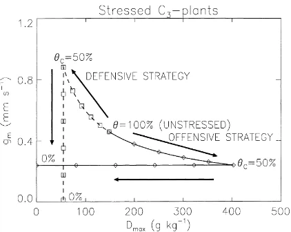
Fig. 4. The response to soil water stress of plants following an offensive strategy, using the A–gsmodel. The mesophyll conductance gm
is given as a function of the maximum leaf-to-air saturation deficit Dmax, in stressed and unstressed conditions. Values of gmand Dmax
were obtained by optimising the A–gs model for several classes of decreasing extractable soil water contentθ or soil water potentialψ,
according to (sunflower — Turner et al., 1984, 1985, hazel tree — Farquhar et al., 1980) leaf or (MUREX — Calvet et al., 1999) field estimates of stomatal conductance as a function of leaf-to-air, or canopy-to-air saturation deficit, respectively.
drought-driven trajectories in the gm–Dmax space is
indicated according to the extractable soil moisture or to the soil water potential. The stress responses are noticeably different among the studied plant species. However, two prevailing behaviours are observed: (1) sunflower, hazel tree, and the MUREX fallow (Fig. 4) undergo a decrease in gmand an increase in Dmax
dur-ing the first stage of soil water depletion; then Dmax
decreases rapidly at fairly constant values of gm
(ex-cept for sunflower, the gm of which ends up
decreas-ing when the soil becomes very dry); (2) conversely, the cowpea and soybean crops (Fig. 5) present an in-crease in gmand a decrease in Dmaxfor moderate soil
desiccation, and a decrease in gm over a small range
of Dmax for more pronounced soil dryness. It is
in-teresting to note that for both strategies, the gm–Dmax
response to the first stage of water stress is almost parallel to the C3-line of Fig. 3 (see Section 6.1).
5.2. The stressed parameters of the Ts-based Jarvis approach
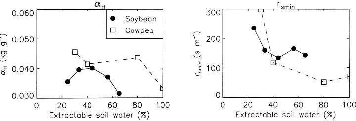
Figs. 6 and 7 present the results obtained using the Ts-based Jarvis approach. In this case, the model
Fig. 5. The response to soil water stress of plants following a defensive strategy, using the A–gs model. The mesophyll conductance gm
is given as a function of the maximum leaf-to-air saturation deficit Dmax, in stressed and unstressed conditions. Values of gmand Dmax
were obtained by optimising the A–gs model for several classes of decreasing extractable soil water contentθ according to (Cowpea —
Hall and Schulze, 1980) leaf or (Soybean — Olioso et al., 1996) field estimates of stomatal conductance as a function of leaf-to-air, or canopy-to-air saturation deficit, respectively.
a function ofθ because no simple relationship could be found between either rsmin and αH or rsmin−1 and
α−H1. However, the main conclusions obtained with the A–gsparameters concerning the stomatal sensitivity to
Ds (represented here by the parameterαH) are
con-firmed. Sunflower, hazel tree, and the MUREX fallow (Fig. 6) show lower values ofαHfor intermediate soil
moisture, while the opposite behaviour is observed for cowpea and soybean (Fig. 7).
Fig. 6. The response to soil water stress of plants following an offensive strategy, using the Ts-based Jarvis approach. The leaf sensitivity
to leaf-to-air saturation deficit (αH, left), and the minimum stomatal resistance (rsmin, right) are plotted vs. the extractable soil moisture
θ (Eq. (9)). In the case of hazel tree, soil water potential values (ψ) were converted to θ values by using the arbitrary function θ=(|ψ|−b− |ψ
min|−b)/(|ψmax|−b− |ψmin|−b), with b=3.5,ψmin=−20 bar, andψmax=−13 bar.
5.3. The stressed parameters of the Ta-based Jarvis approach
The results obtained using the Ta-based Jarvis
ap-proach (not shown) show that the general trend of the rsmin andαH response to soil moisture is the same as
in Figs. 6 and 7. However, the evolution of the stom-atal sensitivity to Ds is more complex than the
Fig. 7. The response to soil water stress of plants following a defensive strategy, using the Ts-based Jarvis approach. The leaf sensitivity
to leaf-to-air saturation deficit (αH, left), and the minimum stomatal resistance (rsmin, right) are plotted vs. the extractable soil moistureθ
(Eq. (9)).
Jarvis approach in Figs. 6 and 7. This result indicates that using Ta as a factor of the stomatal aperture is
not fundamentally different from using Ts, but that Ts
seems to be a better descriptor of the temperature de-pendence of the gs parameters.
6. A parameterisation of soil water stress based on theAAA–gggs approach
In Section 5.1, it was shown that the parameters of the A–gsmodel vary along with soil moisture and that
the way this adaptation occurs differs from moderate to strong water stress and from one plant type to another.
6.1. Similarity of stressed and unstressed relationships
The negative correlation found in Section 4 between ln(gm∗) and ln(D∗max) for C4and C3herbaceous plants
may denote a functional adaptation to the environment. Very high values ofDmax∗ , as obtained for a number of species, correspond to little stomatal sensitivity to air humidity. The lack of response of gs to air humidity
may restrict plant survival in dry conditions. In that situation, Fig. 3 attests that gm∗, and hence the gen-eral level of stomatal conductance and photosynthesis (whatever, air humidity) are generally lower. On the other hand, plants showing a high sensitivity to air humidity (that is, closing their stomata rapidly with increasing saturation deficits, consistent with low val-ues ofDmax∗ ), may compensate for the resulting deficit
of photosynthesis through higher values ofgm∗. In this respect, the C4and C3lines of Fig. 3 may correspond
to viable parameters of the photosynthesis in differing environmental conditions.
Rather than proposing a full mechanistic model, the goal of this study is to bring out possible mechanisms of the plant response to drought from available data. The C3-line of Fig. 3 is valid for unstressed conditions
(θ>90%), and is given by
ln(g∗m)=2.381−0.6103 ln(D∗max)
(n=31, r2=0.40) (10) The results obtained in this study for C3 herbaceous
plants suggest that: (1) as shown by Table 5, the correlated variability of thegm∗ andD∗maxparameters (represented by the regression equation (10)) is also observed for well watered plants of the same species grown under different soil substrate, or ‘pot-size’ con-ditions; (2) for extractable soil water content higher than 40%, the plant response to drought is similar to the ‘pot-size’ rooting effect. Indeed, an equation similar to the unstressed gm–Dmax relationship of
Eq. (10) is observed with moderately stressed plants (90%>θ>40%)
ln(gm)=1.130−0.4594 ln(Dmax)
ln(gm)=2.215−0.5944 ln(Dmax)
(n=40, r2=0.40) (12) while a different result is obtained if only stressed data are considered (i.e. 90%>θ>0%)
ln(gm)= −0.291−0.2238 ln(Dmax)
(n=22, r2=0.11) (13) The similarity of the gm–Dmax relationships
ob-tained under unstressed, moderately stressed, and divers ‘pot-size’ conditions may not be fortuitous and the plant response to the early stage of soil desicca-tion may be related to the soil resistance to rooting (which varies according to soil water content). As already mentioned (Section 5.1), increasing, moder-ate soil wmoder-ater stress induces two radically different effects: the plant may react either as it were grown into a ‘smaller pot’, or on the contrary into a ‘larger pot’. In other words, depending on the plant-type (and maybe on the soil type), moderate soil water stress may either trigger root compaction or, on the contrary, stimulate root growth. In the first situation, the stom-atal response to vapour pressure deficit is increased, while the sensitivity to air dryness decreases in the second case. Given the limited number of studies, it is difficult to draw definite conclusions about the effect of the mechanical limitation of rooting on the value of gm∗ and Dmax∗ . However, the effect presented in Table 5 is in agreement with other results showing that various well watered pot-grown plants respond to Ds,
while the same plants grown in well watered natural soils do not (Tardieu and Simonneau, 1998). Specific experiments on the effect of pot size on transpiration showed that there is a reduction of plant transpiration with decreasing pot size (Ray and Sinclair, 1998). Moreover, physiological experiments showed that the resistance that soil exerts to penetration by plant roots may have an influence on the photosynthesis rate (Masle et al., 1990). A consequence of these observations is that the location of the unstressedgm∗
andDmax∗ parameters of a given plant on the C4- or
C3-line of Fig. 1 may depend on soil depth, texture,
density, structure, and presence of stones. Since soil hardness also depends on soil water content, there might be an interaction between the soil water stress and the soil hardness effects on the plant functioning.
This observation may explain reported dissimilarities between past studies (Turner et al., 1984).
Finally, the two responses to stress illustrated by Figs. 4 and 5 may be interpreted as two distinct strate-gies:
1. The growth of the root-system of the plants fol-lowing the first strategy (sunflower, hazel tree, and the MUREX fallow) may be stimulated under mod-erate soil water stress, consistent with a displace-ment towards higher values of Dmaxon the C3-line.
This somewhat ‘offensive’ way to respond to water stress may be related to the ability of these plants to develop a deep root-system (Cabelguenne and De-baeke, 1998). Such a behaviour was described by Reid and Renquist (1997) in the case of field-grown tomatoes. Exploring deeper soil layers may be a way to compensate for the lack of stomatal regu-lation associated with high values of Dmax(Manes
et al., 1997). Also, short-cycled plants may follow such a strategy. In this case, the lack of stomatal control is compensated by a phenological ability to survive drought, either through a rapid reproductive cycle or through underground vegetative elements able to survive water shortage.
2. On the contrary, the ‘defensive’ strategy of cowpea and soybean may be explained by an increased stomatal regulation in response to higher soil hard-ness (appearing in relation to lower soil moisture). Following the C3-line for moderate soil water
stress, that is, improving the assimilation capacity by increasing gm, while saving water by
reduc-ing Dmax, enables the plant to survive drought in
spite of limited water supply and a relatively long growing cycle.
6.2. An empirical response function
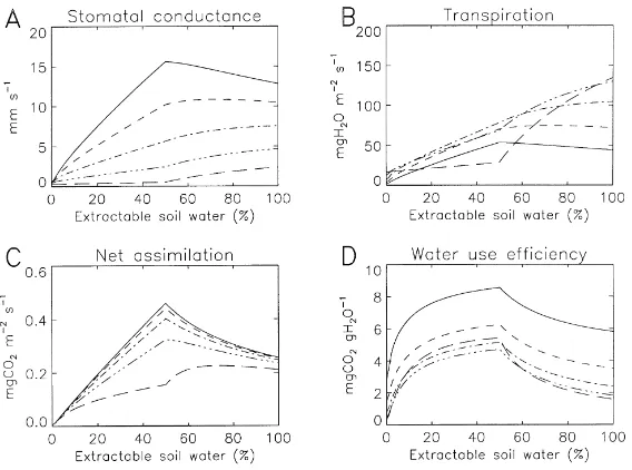
A representation of both offensive and defensive strategies based on the A–gsapproach is given by Figs.
8–10 for C3 plants having the same unstressed
pa-rameters. Schematically, the first phase of soil water stress is represented by a linear response of Dmax to
values of extractable soil waterθ comprised between 100% and a given critical valueθC(an arbitrary value
of 50% is taken in Fig. 8). During this phase, gm is
related to Dmax by the C3-line logarithmic equation.
For values ofθbelowθC, gmand Dmaxare alternately
Fig. 8. Schematic representation of two strategies of C3
plants to adapt the values of mesophyll conductance gm and
maximum leaf-to-air saturation deficit Dmax in response to
soil water stress. In the offensive strategy (solid line, dia-monds) Dmax deviates from its unstressed value Dmax∗ through
Dmax=DmaxX +(D∗max−DmaxX )(θ−θC)/(1−θC), whereDmaxX is
the maximum value of Dmax, for values ofθ lower than the
crit-ical extractable soil moistureθC (that is, for moderate soil water
stress). Meanwhile, gm decreases according to Dmax, following
the C3logarithmic regression equation of Fig. 3. In the defensive
strategy (dashed line, boxes), the same equations are used, where DX
max is replaced byDNmax, the minimum value of Dmax. Below
θC, (i.e. for more pronounced water stress) gm remains constant,
andDmax=DNmax+(DXmax−DNmax)θ/θCin the offensive strategy,
whilegm=gmXθ /θCand Dmaxremains constant in the defensive
strategy (gX
mis the value of gmcorresponding toDNmaxthrough the
C3regression line). As an example, the values ofDNmax,D∗max, and
DX
max, are 55, 148, and 403 g kg−1, respectively, andθC=50%.
offensive and the defensive responses, respectively. The leaf stomatal conductance, transpiration, net as-similation (An), and water use efficiency (WUE), as
calculated by the modified A–gs model as a function
ofθ and Ds, are given in Figs. 9 and 10 for the same
offensive and defensive responses described in Fig. 8, respectively. The water use efficiency WUErepresents
the plant ability to assimilate carbon for a given loss of transpired water.
WUE=
An
E (14)
It clearly appears that the leaf response to soil wa-ter stress sharply depends on the value of Ds. Namely,
there is an interaction between soil and atmospheric water stress. A remarkable difference between offen-sive and defenoffen-sive responses consists in a higher WUE
for intermediate soil water contents in the defensive case, for given Ds conditions, whereas WUE
dimin-ishes in the offensive one. Also, An varies
signifi-cantly according toθand Dsin the defensive response,
while An is much more stable in the offensive one.
This is consistent with different survival mechanisms: (1) water-saving regulation in the defensive strategy (implying a constant adaptation of photosynthesis); (2) weak physiological response to soil water stress, compensated by a more efficient root water-uptake or a more rapid growing cycle in the offensive strat-egy. These results may explain why so many different parameterisations of the soil water stress have been proposed for SVAT-modelling (Mahfouf et al., 1996). Since theθ–Ds interaction is not explicitly treated in
any of them, each parameterisation may result in cor-rect simulations under given Ds conditions, for given
soil and plant-response strategies, but fail elsewhere.
6.3. Application to interactive vegetation modelling
In order to test the suitability of these conclusions, the offensive response displayed in Fig. 8 was applied to the interactive-vegetation simulations performed by the ISBA–A–gs model on the three growing cycles of
Fig. 9. Simulated response of leaf-air exchange variables to soil water stress in the offensive strategy. The simulations are performed using the parameters of Fig. 8, at 30◦C, a solar radiation of 800 W m−2, and CO
2 air concentration of 350 ppm, for leaf-to-air saturation
deficits of 3, 6, 12, 24, and 48 g kg−1 (solid, dashed, dash-dotted, dash-three-dotted, and long-dashed lines, respectively). (A) Leaf stomatal
conductance; (B) leaf transpiration; (C) CO2assimilation and (D) water use efficiency.
Fig. 10. Simulated response of leaf-air exchange variables to soil water stress in the defensive strategy. The simulations are performed using the parameters of Fig. 8, at 30◦C, a solar radiation of 800 W m−2, and CO
2 air concentration of 350 ppm, for leaf-to-air saturation
deficits of 3, 6, 12, 24, and 48 g kg−1 (solid, dashed, dash-dotted, dash-three-dotted, and long-dashed lines, respectively). (A) Leaf stomatal
Fig. 11. Comparison between measurements (boxes and diamonds) performed over the MUREX fallow and simulations (line) of the ISBA–A–gs model (Calvet et al., 1998), accounting for the offensive strategy described in Fig. 8 (the same numerical values are used).
(A) Leaf area index and (B) extractable soil water content.
during this period. A possible explanation may be that the planimetric method employed to estimate LAI fails when many leaves become senescent, because of the difficulty to make the difference between ‘green’ leaf-parts and senescent ones.
7. Discussion
In this study, two types of data are employed: cham-ber or cuvette measurements at the leaf scale, and micrometeorological field measurements characteris-ing a vegetation canopy. One may wonder whether chamber data are of equal value to field data, in terms of accuracy and representativeness. Although the em-ployed datasets represent the current state of the art, both chamber and field data are subjected to measure-ments uncertainties. As shown in this study, both A–gs
and Jarvis parameters may depend on the interaction between roots and the soil substrate. This effect may also be at stake during soil depletion through interac-tions between soil moisture, soil resistance to rooting, and hormonal control of rooting. The field-adaptation which is often observed (e.g. Tardieu and Simonneau, 1998) may be due to this kind of interaction. However,
since obstacles to rooting may also occur in the field, there is no fundamental difference between chamber and field data.
Documenting diversity of local observations may seem contradictory with the objective of improving more general SVAT models. However, it must be un-derlined that the meteorological question considered in this study is not whether a Jarvis or A–gsmodel can
be parameterised for any given situation, but whether the parameters of these models can be estimated us-ing guidelines gained from observable features of the soil–plant–atmosphere system. Figs. 4–8 give a first response to this question by showing the effect of soil moisture on the parameters of commonly used param-eterisations. Of course, there may be an uncertainty in parameter selection. However, the employed A–gs
model (Jacobs et al., 1996) is a simplified parameter-isation using a small number of parameters. Among these parameters, few are expected to be strongly driven by soil water stress. As shown in Appendix A, the basic variables employed to describe net as-similation and stomatal conductance are maximum photosynthesis Am (Eq. (A.1)) and intercellular CO2
concentration Ci (Eq. (A.2)). These variables depend
Table 6
Comparison of the gm–Dmaxand gm–f0analyses in terms of average RMS error on the stomatal conductance (gs′) of the micrometeorological
measurements of MUREX (Calvet et al., 1999) and the Soybean field (Olioso et al., 1996) Variables RMS error on MUREXg′
s (mm s−1) RMS error on the soybean fieldg′s (mm s−1)
gm–Dmax 1.2 0.4
gm–f0 1.3 0.7
shown in Appendix A, the f0 parameter represents
a potential value of the Ci/Cs ratio. In this study, it
was assumed that gm and Dmax may vary according
to soil moisture, while f0 is prescribed (Table 1).
Also, tests were made assuming stress-dependent gm
and f0, with a constant value Dmax=45 g kg−1.
Sim-ilar to the gm–Dmax analysis presented in Sections 4
and 5, good correlations were obtained between the unstressed gm and f0, and two opposite behaviours
were observed in conditions of stress (not shown). However, the gm–Dmax analysis is more efficient to
describe the observations as shown by Table 6. In this study, two types of parameterisations are considered: Jarvis and A–gs. The Jarvis model is
clearly a phenomenological approach which does not pretend to describe the mechanism of the stomatal re-sponse. Multiplying maximum stomata conductance by an empirical soil water function is perfectly consis-tent with this approach (Noilhan and Planton, 1989). On the other hand, the A–gs model describes the
in-teraction between carbon uptake, transpiration and stomatal aperture in a more mechanistic way. Calvet et al. (1998) employed a phenomenological approach to describe soil water stress in an A–gsmodel: the
un-stressed mesophyll conductancegm∗ is multiplied by the normalised extractable soil water. Although there is a contradiction between incorporating soil water stress via a phenomenological approach in an A–gs
model, which is mechanistic by nature, this pragmatic solution was chosen because the employed A–gs
model (Jacobs et al., 1996) did not include a represen-tation of soil water stress, and because it was the most obvious way to do so. Nonetheless, this first order rep-resentation of water stress was very efficient to simu-late the water balance of the six sites studied by Calvet et al. (1998). Here, an attempt is made to investigate whether a more mechanistic description of the stressed parameters would be useful. The fact that the soil wa-ter stress effect presented in Figs. 4–7 is all the more apparent since the model is more mechanistic (the
A–gs approach seems to be superior to the Ts-based
Jarvis one, and the Ts-based Jarvis to the Ta-based one)
confirms that it is possible to go further into the com-prehension of the phenomena by using available data. Regarding more mechanistic descriptions of stress, physiologists have often proposed to use a plant hydraulic model to make a connection to soil water potential (e.g. Tardieu and Simonneau, 1998). Param-eterisations of chemical signalling from roots to leaves were coupled to this kind of models. Nevertheless, the use of soil water potential (ψ) is controversial. A number of past and recent findings indicate that the (apparently) more mechanistic approach of using a plant hydraulic model to make a connection toψmay not be adequate. SVAT models’ intercomparison made by meteorologists (e.g. Mahfouf et al., 1996; Chen et al., 1997) show that models using the notion of soil
ψdo not surpass those employing simple parameter-isations based on bulk soil moisture. In some cases, these simple models outdo ψ models (Calvet et al., 1999). During the past decade, physiologists have presented results confirming this view. Although ψ
models accounting for hormonal drought signal were developed, the role of water relations and hormonal signals in the plant response to drought are still un-clear (e.g. Socias et al., 1997). In particular, the xylem sap hormonal or pH response to soil water stress may occur before any change in soil or leafψ is detected, and in many cases soil water content is a much more sensitive indicator of soil dryness effects (Turner et al., 1985; Schulze, 1986; Garnier and Berger, 1987; Kopka et al., 1997; Wilkinson et al., 1998; Ali et al., 1999).
8. Conclusion
To some extent, this study raises as many questions as it answers. This is a first step to better understand the response of plant stomata to atmospheric humidity and soil water availability. Further works should focus on obtaining more general SVAT models based on these results. The main results are the following:
• The intraspecific variability of either Jarvis or A–gs
unstressed parameters is as large as the interspecific variability. Soil resistance to rooting seems to be a factor of the intraspecific differences.
• Jarvis and A–gs approaches present rather similar
responses to soil water stress.
• The stomatal sensitivity to air humidity seems to be conditioned by the soil water content.
• Several strategies (at least two) may explain changes in stomatal conductance induced by soil water de-pletion. More fundamental research is needed to understand the action of soil moisture on rooting and why both offensive and defensive strategies are observed. Possibly, a mechanistic model could then be proposed.
• Field studies are consistent with the results obtained at the leaf scale.
Acknowledgements
The author wishes to thank Drs. J. Noilhan and C. Hoff (CNRM), P. Mordelet (CESBIO), A. Olioso, J.-P. Wigneron, and B. Itier (INRA), as well as the anony-mous reviewers, for comments, advice and discussion.
Appendix A. TheAAA–gggsmodel
The A–gs approach employed to describe the
leaf-scale physiological processes in ISBA–A–gs (Calvet
et al., 1998) was the model proposed by Jacobs et al. (1996).
The photosynthesis rate in light-saturating condi-tions is expressed as
The gm∗ parameter (the unstressed mesophyll con-ductance) is corrected for leaf temperature using a Q10-type function, together with the maximum
photo-synthesis Am,maxand the compensation pointŴ.
Typ-ical values of Am,maxandŴat a temperature of 25◦C,
for C3 and C4plants, are given in Table 1. To avoid
lengthy iterations, the internal CO2 concentration Ci
is obtained by combining the air CO2 concentration
CsandŴthrough the following closure equation:
Ci=fCs+(1−f )Ŵ (A.2)
where the coupling factor f is sensitive to air humidity and depends on the cuticular conductance gc and on
bothgm∗ andD∗maxby
1). The net assimilation is limited by a light deficit according to a saturation equation applied to the photosynthetically active radiation Ia:
An=(Am+Rd)
2Ŵ), whereε0is the maximum quantum use efficiency
(Table 1). Finally,
where Aminrepresents the residual photosynthesis rate
(at full light intensity) associated with cuticular trans-fers when the stomata are closed because of a high saturation deficit.
Ali, M., Jensen, C.R., Mogensen, V.O., Bahrun, A., 1999. Drought adaptation of field grown wheat in relation to soil physical conditions. Plant and Soil 208, 149–159.
Attiwill, P.M., Squire, R.O., Neales, T.F., 1982. Photosynthesis and transpiration of Pinus radiata D. Don under plantation conditions in Southern Australia. II. First year seedlings and 5-year-old tree on aeolian sands at Rennick (south-western Victoria). Aust. J. Plant Physiol. 9, 761–771.
Bakker, J.C., 1991. Leaf conductance of four glasshouse vegetable crops as affected by air humidity. Agric. For. Meteorol. 55, 23–36.
Bunce, J.A., 1985. Effect of boundary layer conductance on the response of stomata to humidity. Plant, Cell Environ. 8, 55–57. Cabelguenne, M., Debaeke, P., 1998. Experimental determination and modelling of the soil water extraction capacities of crops of maize, sunflower, soya bean, sorghum and wheat. Plant and Soil 202, 175–192.
Calvet, J.-C., Noilhan, J., Roujean, J.-L., Bessemoulin, P., Cabelguenne, M., Olioso, A., Wigneron, J.-P., 1998. An interactive vegetation SVAT model tested against data from six contrasting sites. Agric. For. Meteorol. 92, 73–95.
Calvet, J.-C., Bessemoulin, P., Noilhan, J., et al., 1999. MUREX: a land-surface field experiment to study the annual cycle of the energy and water budgets. Ann. Geophysicae, 17, 838–854. Chen, T.H., Henderson-Sellers, A., Milly, P.C.D., Pitman,
A.J., Beljaars, A.C.M., et al., 1997. Cabauw experimental results from the project for intercomparison of landsurface parameterization schemes. J. Clim. 10 (7), 1194–1215. Choudhury, B.J., Monteith, J.L., 1986. Implications of stomatal
response to saturation deficit for the heat balance of vegetation. Agric. For. Meteorol. 36, 215–225.
Cohen, S., Cohen, Y., 1983. Field studies of leaf conductance response to environmental variables in Citrus. J. Appl. Ecol. 20, 561–570.
Collatz, G.J., Ball, J.T., Grivet, C., Berry, J.A., 1991. Physiological and environmental regulation of stomatal conductance, photosynthesis and transpiration: a model that includes a laminar boundary layer. Agric. For. Meteorol. 54, 107–136. Comstock, J., Ehleringer, J., 1993. Stomatal response to
humidity in common bean (Phaseolus vulgaris): implications for maximum transpiration rate, water-use efficiency and productivity. Aust. J. Plant Physiol. 20, 669–691.
Cowan, I.R., 1982. Regulation of water use in relation to carbon gain in higher plants. In: Lange, O.L., Nobel, P.S., Osmond, C.B., Ziegler, H. (Eds.), Encyclopedia of Plant Physiology, New Series, Vol. 12B, Physiological Plant Ecology II. Springer, Berlin, pp. 589–615.
Dai, Z., Edwards, G.E., Ku, M.S.B., 1992. Control of photosynthesis and stomatal conductance in Ricinus communis L. (Castor Bean) by leaf to air vapor pressure deficit. Plant Physiol. 99, 1426–1434.
De Rosnay, P., 1999. Représentation de l’interaction sol-végétation-atmosphère dans le modèle de circulation générale du CMD. Ph.D. Thesis, Université Paris 6, Paris 176 pp.
Dickinson, R.E., Shaikh, M., Bryant, R., Graumlich, L., 1998. Interactive canopies for a climate model. J. Clim. 11, 2823–2836.
Dufrene, E., Saugier, B., 1993. Gas exchange of oil palm in relation to light, vapour pressure deficit, temperature and leaf age. Funct. Ecol. 7, 97–104.
El-Sharkawy, M.A., Cock, J.H., Held, K.A.A., 1984. Water use efficiency of Cassava. II. Differing sensitivity of stomata to air humidity in Cassava and other warm-climate species. Crop Sci. 24, 503–507.
Farquhar, G.D., Schulze, E.-D., Küppers, M., 1980. Responses to humidity by stomata of Nicotinia glauca L. and Corylus avellana L. are consistent with the optimisation of carbon dioxide uptake with respect to water loss. Aust. J. Plant Physiol. 7, 315–327.
Farquhar, G.D., Wong, S.C., Evans, J.R., Hubick, K.T., 1989. Photosynthesis and gas exchange. In: Hamlyn, G.J., Flowers, T.L., Jones, M.B. (Eds.), Plants Under Stress. Biochemistry, Physiology and Ecology and Their Application to Plant Improvement. Cambridge University Press, Cambridge, pp. 47–69.
Garnier, E., Berger, A., 1987. The influence of drought on stomatal conductance and water potential of peach trees growing in the field. Scientia Horticulturae 32, 249–263.
Graham, M.E.D., Thurtell, G.W., 1989. The effect of increased transpiration on photosynthesis of corn. II. Comparisons between hydroponically and soil-grown plants. Agric. For. Meteorol. 44, 317–328.
Grantz, D.A., Meinzer, F.C., 1990. Stomatal response to humidity in a sugarcane field: simultaneous porometric and micrometeorological measurements. Plant, Cell Environ. 13, 27–37.
Gucci, R., Massai, R., Xiloyannis, C., Flore, J.A., 1996. The effect of drought and vapour pressure deficit on gas exchange of young Kiwifruit (Actinidia deliciosa var. deliciosa) vines. Ann. Bot. 77, 605–613.
Hall, A.E., Schulze, E.-D., Lange, O.L., 1976. Current perspectives of steady state stomatal responses to environment. In: Lange, O.L., Kappen, L., Schulze, E.-D. (Eds.), Water and Plant Life. Springer, New York, pp. 169–188.
Hall, A.E., Schulze, E.-D., 1980. Stomatal response to environment and a possible interrelation between stomatal effects on transpiration and CO2 assimilation. Plant, Cell Environ. 3,
467–474.
Jacobs, C.M.J., 1994. Direct impact of atmospheric CO2
enrichment on regional transpiration. Ph.D. Thesis, Agricultural University, Wageningen, 179 pp.
Jacobs, C.M.J., van den Hurk, B.J.J.M., de Bruin, H.A.R., 1996. Stomatal behaviour and photosynthetic rate of unstressed grapevines in semi-arid conditions. Agric. For. Meteorol. 80, 111–134.
Ji, J.J., 1995. A climate-vegetation interaction model: simulating physical and biological processes at the surface. J. Biogeogr. 22, 445–451.
Jolliet, O., Bailey, B.J., 1992. The effect of climate on tomato transpiration in greenhouses: measurements and models comparison. Agric. For. Meteorol. 58, 43–62.
Kawamitsu, Y., Yoda, S., Agata, W., 1993. Humidity pretreatment affects the responses of stomata and CO2assimilation to vapor
pressure difference in C3 and C4 plants. Plant Cell Physiol.
34 (1), 113–119.
Kopka, J., Provart, N.J., Muller-Rober, B., 1997. Potato guard cells respond to drying soil by a complex change in the expression of genes related to carbon metabolism and turgor regulation. Plant J. 11 (4), 871–882.
Mahfouf, J.-F., Ciret, C., Ducharne, A., Irannejad, P., Noilhan, J., et al., 1996. Analysis of transpiration from the RICE and PILPS workshop. Global Planet. Change 13, 73–88.
Manes, F., Seufert, G., Vitale, M., 1997. Ecophysiological studies of Mediterranean plant species at the Castelporziano estate. Atmos. Environ. 31 (S1), 51–60.
Maroco, J.P., Pereira, J.S., Chaves, M.M., 1997. Stomatal responses to leaf-to-air vapour pressure deficit in Sahelian species. Aust. J. Plant Physiol. 24, 381–387.
Masle, J., Farquhar, G.D., Gifford, R.M., 1990. Growth and carbon economy of wheat seedlings as affected by soil resistance to penetration and ambient partial pressure of CO2. Aust. J. Plant
Physiol. 17, 465–487.
Meinzer, F.C., 1982. The effect of vapour pressure on stomatal control of gas exchange in Douglas fir (Pseudotsuga menziesii) saplings. Oecologia (Berlin) 54, 236–272.
Monteith, J.L., 1995. A reinterpretation of stomatal responses to humidity. Plant, Cell Environ. 18, 357–364.
Morison, J.I.L., Gifford, R.M., 1983. Stomatal sensitivity to carbon dioxide and humidity. A comparison of two C3 and two C4
grass species. Plant Physiol. 71, 789–796.
Mott, K.A., Parkhurst, D.F., 1991. Stomatal response to humidity in air and helox. Plant, Cell Environ. 14, 509–515.
Noilhan, J., Planton, S., 1989. A simple parameterization of land surface processes for meteorological models. Mon. Wea. Rev. 117, 536–549.
Olioso, A., Carlson, T.N., Brisson, N., 1996. Simulation of diurnal transpiration and photosynthesis of a water stressed soybean crop. Agric. For. Meteorol. 81, 41–59.
Ray, J.D., Sinclair, T.R., 1998. The effect of pot size on growth and transpiration of maize and soybean during water deficit stress. J. Exp. Bot. 49 (325), 1381–1386.
Reid, J.B., Renquist, A.R., 1997. Enhanced root production as a feed-forward response to soil water deficit in field-grown tomatoes. Aust. J. Plant Physiol. 24, 685–692.
Schulze, E.-D., 1986. Carbon dioxide and water vapor exchange in response to drought in the atmosphere and in the soil. Ann. Rev. Plant Physiol. 37, 247–274.
Sellers, P.J., Mintz, Y., Sud, Y.C., Dalcher, A., 1986. A simple biosphere model (SiB) for use within general circulation models. J. Atmos. Sci. 43 (6), 505–531.
Shuttleworth, W.J., 1989. Micrometeorology of temperate and tropical forest. Philos. R. Trans. Soc., London B324, 299–334. Socias, X., Correia, M.J., Chaves, M., Medrano, H., 1997. The role of abscissic acid and water relations in drought responses of subterranean clover. J. Exp. Bot. 48 (311), 1281–1288. Tardieu, F., Simonneau, T., 1998. Variability among species
of stomatal control under fluctuating soil water status and evaporative demand: modelling isohydric and anisohydric behaviours. J. Exp. Bot. 49, 419–432.
Thorpe, M.R., Warrit, B., Landsberg, J.J., 1980. Response of apple leaf stomata: a model for single leaves and a whole tree. Plant, Cell Environ. 3, 23–27.
Turner, N.C., Schulze, E.-D., Gollan, T., 1984. The responses of stomata and leaf gas exchange to vapour pressure deficits and soil water content. I. Species comparisons at high soil water contents. Oecologia (Berlin) 63, 338–342.
Turner, N.C., Schulze, E.-D., Gollan, T., 1985. The responses of stomata and leaf gas exchange to vapour pressure deficits and soil water content. II. In the mesophytic herbaceous species Helianthus annuus. Oecologia (Berlin) 65, 348–355. Wilkinson, S., Corlett, J.E., Oger, L., Davies, W.J., 1998. Effects
of xylem pH on transpiration from wild-type and flacca tomato leaves. A vital role for abscissic acid in preventing excessive water loss even from well-watered plants. Plant Physiol. 117, 703–709.
Will, R.E., Teskey, R.O., 1997. Effect of irradiance and vapour pressure deficit on stomatal response to CO2 enrichment of