3D BUILDING ADJUSTMENT
USING PLANAR HALF-SPACE REGULARITIES
Andreas Wichmann, Martin Kada
Institute for Geoinformatics and Remote Sensing (IGF), University of Osnabrück Barbarastr. 22b, 49076 Osnabrück, Germany
Commission III, WG IV
KEY WORDS: Reconstruction, Three-dimensional, Building, Modelling, Adjustment, Feature, Rectification, Point Cloud
ABSTRACT:
The automatic reconstruction of 3D building models with complex roof shapes is still an active area of research. In this paper we present a novel approach for local and global regularization rules that integrate building knowledge to improve both the shape of the reconstructed building models and their accuracy. These rules are defined for the planar half-space representation of our models and emphasize the presence of symmetries, co-planarity, parallelism, and orthogonality. By not adjusting building features separately (e.g. ridges, eaves, etc.) we are able to handle more than one feature at a time without considering dependencies between different features. Additionally, we present a new method for reconstructing buildings with concave outlines using half-spaces that avoids the need to partition the models into smaller convex parts. We present both extensions in the context of a fully automatic feature-driven 3D building reconstruction approach where the whole process is suited for processing large urban areas with complex building roofs.
1. INTRODUCTION
The automatic reconstruction of 3D building models with detailed roof structures in urban areas that are suitable for analysis tasks and are not restricted to visualization purposes is still an active research area. Several reconstruction approaches based on LIDAR data have been developed in the past two decades (Brenner, 2010; Haala and Kada, 2010; Rottensteiner et al., 2012). According to Tarsha-Kurdi et al. (2007) these reconstruction approaches can generally be characterized as either model-driven (top-down) or data-driven (bottom-up).
In model-driven approaches building templates are chosen from a predefined catalog and then adapted by their parameters to best fit their roof shapes to the given data (Maas and Vosselman, 1999). An advantage of these reconstruction approaches is that they always generate topologically correct building models even if the data is of lower point density. The parameterization of the building templates insures that the reconstructed models are always well-shaped. The limitation of model-driven approaches is that only those building shapes can be reconstructed which are already included in the predefined catalog.
To avoid extensive catalogs for the reconstruction of complex building models data-driven methods have been developed. These bottom-up approaches start with a segmentation to obtain sets of points which usually determine planar regions representing roof faces. There exist several methods for segmentation like Hough Transform (Overby et al., 2004; Oda et al., 2004), RANSAC (Tarsha-Kurdi et al., 2008), and region growing (Alharthy and Bethel, 2004; Rottensteiner, 2003). The segments are then combined e.g. by plane intersection and step edge detection to determine their boundaries (Rottensteiner, 2005). Additionally, the building outline has to be determined.
There exist several methods which do not require additional building data (Neidhart and Sester, 2008; Sampath and Shan, 2007). By combining the roof planes with the building outline a 3D building model is constructed.
The main common difficulty of these data-driven approaches is that the local plane fitting and the determination of the building outline become unstable for noisy point clouds and segments with a small number of points. In contrast to model-driven approaches this often leads to unnatural structures in the resulting models and decreases their natural regularities and symmetries. There exist only few methods that modify misaligned planes and outlines for building reconstruction purposes which avoid these disadvantages. Some of them use line simplification methods that take parallel and orthogonal structures together with the main building orientation into account (Vosselman, 1999; Alharthy and Bethel, 2004). This way, the process is extended by incorporating additional building knowledge to improve the shape of the reconstructed building models while still keeping the flexibility of a data-driven approach.
Adjustment methods for building models are often performed locally. Complex roof shapes for example are partitioned into sets of simpler roof shapes and the regularization rules are then performed on each individually. Recent methods have shown that also global regularities can significantly improve the modeling quality in terms of fitting accuracy and human vision judgment (Zhou and Neumann, 2012). Like other global restrictions regularization rules are based on the adjustment of single low-level feature types (e.g. ridges, eaves, etc.) which therefore have to be performed on every low-level feature type separately.
In this paper we extend the fully automatic feature-driven building reconstruction approach introduced by Kada and Wichmann (2013) in order to improve the local and global features of the already well-shaped and oriented building models. We perform local and global adjustments on the half-spaces that are defined by high-level features (gable roof, hip roof, mansard roof, gambrel roof, etc.) and roof structures (chimney, dormer, decks, etc.). For an in-depth explanation of half-spaces and half-space modeling see e.g. (Mäntylä, 1988) or (Foley et al., 1990). In contrast to other adjustment methods we are thus able to rectify more than one low-level feature at the same time. Therefore, our regularization rules are also suited for the automatic reconstruction of large urban areas. The local and global regularization rules employed in this paper are based on methods presented in (Thrun and Wegbreit, 2005) and (Li et al., 2011) and modified for building reconstruction purposes.
Additionally, we extend the previously suggested feature recognition step by allowing certain parts of some low-level features to have in certain cases other parameter values than the rest of the feature. The advantage of this extension is that we are able to reconstruct high-level features like gable or hip roofs with concave building outlines by sets of half-spaces. This reduces the number of components of a concave building. Furthermore, we can perform our regularization rules either on certain parts of a low-level feature or on all its parts at the same time.
2. RECONSTRUCTION PROCESS
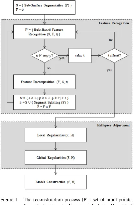
In this section we give a brief overview of the reconstruction process presented in (Kada and Wichmann, 2013) and describe the changes and enhancements introduced in this paper. The process is presented in Figure 1 and consists of the following four steps: sub-surface segmentation, feature recognition, half-space adjustment, and model construction.
In the first step we perform sub-surface segmentation as introduced in (Kada and Wichmann, 2012). In contrast to other region growing segmentation algorithms the segments are enlarged with virtual points that geometrically fit the criteria of the segments, but are located below real surface points as shown in Figure 2. The advantage of introducing sub-surface points is that small segment patches – that are otherwise disconnected because of superstructures – are merged to larger segments and thereby improving the recognition of adjacencies, intersections, and sub-shapes of building roofs.
In the next step the iterative feature recognition introduced in (Kada and Wichmann, 2013) is modified by omitting the feature adjustment and adding a feature decomposition. It starts with a rule-based feature recognition that tries to find as many features as possible matching the feature recognition rules. Some of the newly found features are then decomposed if necessary (see section 5). This allows us to model some buildings with concave outlines without partitioning them into smaller convex components. Afterwards, segments are split when not all surface points are represented by features. This sub-step is implemented by a cloning and reclassification process with regard to surface and sub-surface points. Finally the feature recognition starts again. If no further feature is found some of the thresholds are relaxed. This step ends if the thresholds reach their limit and no further features are found.
Figure 1. The reconstruction process (P = set of input points, S = set of segments, F = set of features, H = set of half-spaces, t = thresholds for feature recognition).
Figure 2. Segmentation of planar regions as a result of surface growing (left) and sub-surface growing (right).
The third step is the newly introduced half-space adjustment that improves the regularities between features. As described by Kada and Wichmann (2013), certain features define planar half-spaces whose intersections produce convex building components. As illustrated in Figure 3 a pitched roof building can be represented as the intersection of seven planar half-spaces. Their adjustment with regard to the geometries of features, their symmetries and regularities results in well-shaped reconstruction models. To ensure that the segments defining a building component have a higher impact on its half-spaces ISPRS Annals of the Photogrammetry, Remote Sensing and Spatial Information Sciences, Volume II-3, 2014
than the segments of other building components we distinguish between local adjustments (see section 3) and global adjustments (see section 4).
Figure 3. Pitched roof building with a ridge feature (green line), two gable features (blue dots), and corresponding half-spaces.
By performing the adjustment on half-spaces instead of on low-level features we are able to adjust more than one low-low-level feature of a building component at the same time. For example, the length of a pitched roof as shown in Figure 3 can be changed easily by translating the half-space H5 or H6. All features of the building like ridge and eaves are automatically adjusted correctly by this translation. In contrast to a feature based adjustment we do not have to consider the dependencies between different features.
In the last step of the reconstruction process 3D building models are constructed using planar half-spaces as described in (Kada and Wichmann, 2013).
3. LOCAL HALF-SPACE ADJUSTMENT
In this section we present the central concept for the local adjustment of half-spaces. We call a half-space adjustment local if the adjustment is performed only on the half-spaces defining a building component and not on other half-spaces. For the local half-space adjustment step we observe that man-made objects like buildings often possess components that are symmetric and regular (Rosen, 1975). To support the occurrence of symmetries and regularities our half-space adjustment of a building component consists roughly of the following three steps:
1. Slope adjustment: a group of half-spaces that feature similar slopes are adjusted to their average value. 2. Orientation adjustment: a group of half-spaces that
feature similar x-y directions are adjusted to their average angular value. Here, we regard orientation as the 2D rotation around the z axis.
3. Position adjustment: vertical half-spaces are shifted to improve symmetries and regularities.
Slope and orientation adjustment are accomplished by similar procedures and are therefore explained together in subsection 3.1. Thereafter, position adjustment is explained in subsection 3.2.
3.1 Slope and orientation adjustment
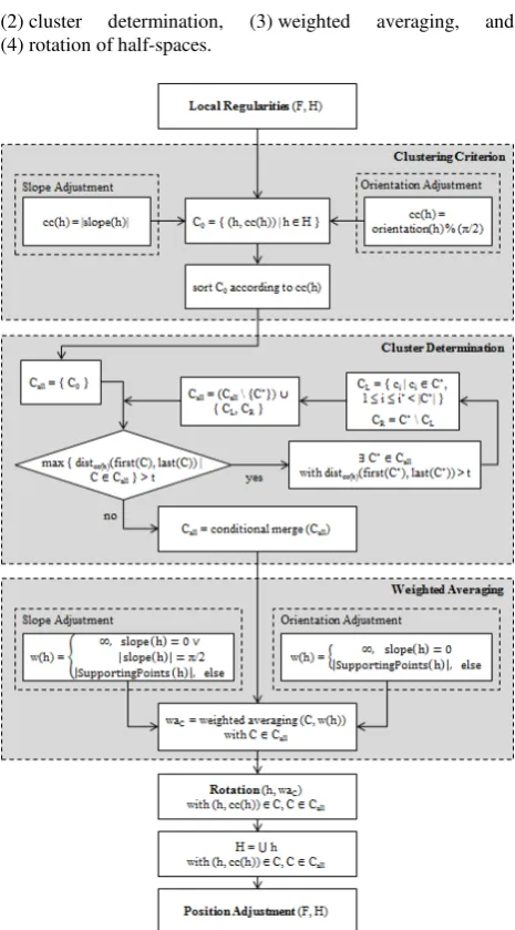
The substantial aspect of slope and orientation adjustment is a clustering of half-spaces. The scheme is presented in Figure 4 and consists of the following four sub-steps: (1) calculation of clustering criterion and sorting of half-spaces accordingly,
(2) cluster determination, (3) weighted averaging, and (4) rotation of half-spaces.
Figure 4. The local half-space adjustment process (F = set of features, H = set of spaces, C = cluster of half-spaces. t = threshold for cluster determination).
To support the occurrence of symmetry we use the absolute values of half-space slopes as clustering criterion of the slope adjustment. Thereby we take into account that for example the two roof top half-spaces of a gable roof often have the same absolute slope value but are pointed in opposite directions. And to support parallelism and orthogonality we use as clustering criterion of the orientation adjustment the orientation angle modulo π/2. The orientation angle is given by the counterclockwise angle between the x-axis and the normal vector of the half-space projected onto the x-y plane. For each local half-space adjustment step we sort all half-spaces according to the respective clustering criterion.
For the subsequent clustering of half-spaces there already exist several general clustering methods (Gan et al., 2007). For our purpose we implement a divisive method that starts with one sorted cluster including all half-spaces. If the distance between the first and the last element of a cluster is greater than a predefined threshold then the cluster is split into two parts between the two adjacent elements that have the greatest ISPRS Annals of the Photogrammetry, Remote Sensing and Spatial Information Sciences, Volume II-3, 2014
distance to each other. The algorithm is recursively applied to the two parts until no further split is necessary, i.e. when the distance between the first and the last element of each cluster is not greater than a predefined threshold. In order to reduce the number of clusters caused by noisy data a conditional merge is performed on the clusters so obtained. A cluster is considered to be isolated if it contains only one half-space estimated by points whose average distance to the plane defining the half-space is greater than a predefined threshold. Every isolated cluster is merged with the nearest adjacent non-isolated cluster and its number of supporting points is set to zero.
After clusters are determined in this way the calculation of the weighted average value for each cluster is performed by taking into account the number of points that support a half-space, i.e. are close to the half-space. In order to maintain the slopes of vertical and horizontal half-spaces in the slope adjustment step we assign to these half-spaces an infinite weight. This has the effect that sloped half-spaces are adjusted towards the vertical and horizontal half-spaces in the next sub-step and not the other way round. In contrast to this we assign in the orientation adjustment a zero weight to all vertical half-spaces. Since the half-spaces in the slope adjustment are sorted according to the absolute values of their slopes there are for every cluster two possible slopes differing only in their sign. Similarly, since the orientation of the half-spaces in the orientation adjustment are taken modulo π/2 there are for every cluster four possible orientation values. For the subsequent rotation of the half-spaces the most probable value of the slope, respectively orientation, is chosen.
For the rotation of a half-space in the slope and the orientation adjustment we define for each step a rotation axis. For the slope adjustment we chose a horizontal line whose direction is orthogonal to the normal vector of the half-space. For the orientation adjustment we chose a vertical line. We chose these two lines so that they have an intersection point which satisfies the following conditions:
• For any non-vertical half-space the intersection point of the two lines is the center point of the segment originally defining the half-space. Therefore, this point is always unaltered by the local half-space adjustment.
• For any vertical half-space the intersection point of the two lines is the center point of the feature. E.g. the intersection point of the two lines for a shed roof is the intersection point of the two lines of the roof top half-space, and for a gable roof it is the center point of its ridge.
The horizontal and the vertical line chosen in this way are taken respectively as the rotation axis in the last sub-step.
3.2 Position adjustment
In the position adjustment, vertical half-spaces are translated along their normal vector to improve symmetries and regularities. It is divided into two sub-steps. First, all vertical half-spaces are sorted by their clustering criterion which is the shortest distance to the feature (e.g. a ridge line) that originally defines the half-space. Then clusters are determined and for each cluster a weighted average distance calculated. Thereafter, all half-spaces are translated along their normal vector so that their shortest distance to the feature corresponds to the
calculated weighted average distance of the cluster to which they belong. If more than one position is possible the position nearest to the original is taken.
We consider in the second sub-step all those pairs of adjacent spaces which consist of a vertical and a non-vertical half-space that intersect in a horizontal line – among others, such a line could be an eave. Two half-spaces are called adjacent if a sufficient number of their points support the intersection, i.e. are close to the intersection line. These half-space pairs are clustered according to the height of their horizontal intersection lines. Now in order to reduce the number of different intersection heights we translate the vertical half-spaces in a cluster along their direction within a strict predefined threshold.
The advantage of carrying out these two sub-steps of the position adjustment is the following:
• The first sub-step ensures that e.g. eaves can be assigned the same height in the second sub-step even if the angle between the two half-spaces belonging to the eave is close to 0.
• The threshold in the second sub-step prevents a vertical half-space to be translated too far away from its original position if the angle between the two adjacent half-spaces of a pair is close to π/2.
Other approaches often directly adjust eave heights without considering the context of how they were generated. The effects are that heights of eaves which are actually of the same height are not adjusted in the model and that features might get shifted too far away.
The impact of the whole local half-space adjustment presented in this paper is illustrated exemplarily on a half-hip building in Figure 5. The roof faces are strictly oriented orthogonal or opposite to each other; opposite faces have the same slope. The ridge and eave lines are horizontal where the latter feature the same height on both sides. So there is symmetry with respect to a vertical plane which passes through the ridge.
Figure 5. Reconstructed building model before (left) and after the local half-space adjustment step (right).
4. GLOBAL HALF-SPACE ADJUSTMENT
As described in the previous section, local half-space adjustment is performed for every building component individually and independently from other components. This allows the use of rules with soft thresholds to support local regularities. In the global half-space adjustment we take care of the global regularities and symmetries which are usually also present in man-made objects (Kazhdan et al., 2004). E.g. two adjacent gable roofs can share the same ridge line as shown in Figure 6. Therefore, the aim of the global half-space adjustment is to adjust the half-spaces of building components in order to ISPRS Annals of the Photogrammetry, Remote Sensing and Spatial Information Sciences, Volume II-3, 2014
support the occurrence of global regularities and symmetries between them while maintaining the local regularities and symmetries within each component as far as possible. This step automatically eliminates global asymmetries caused by the previous local half-space adjustment step. The following four steps roughly illustrate our implementation of the global half-space adjustment procedure:
1. Global slope adjustment performed on the half-spaces of all building components analogous to the local slope adjustment described in section 3, but with a stricter threshold.
2. Global orientation adjustment performed on the half-spaces of all building components analogous to the local orientation adjustment described in section 3, but with a stricter threshold.
3. Feature growing translates half-spaces of building components within a strict predefined threshold so that features are merged.
4. Consider for each orientation the set of all vertical half-spaces having this direction, sort each set by their distance to a fixed point, e.g. the origin, and find clusters. Calculate for each cluster a weighted average and translate each half-space in the cluster along its normal vector according to the calculated average.
In Figure 6 an example of a reconstructed 3D model is shown where the local half-space adjustment of each component has produced several global asymmetries. For example the half-spaces belonging to the left top of the gable roof have different normal vectors and distances to the origin which were originally the same. In this case the first and the second step of the global half-space adjustment restore the original number of different normal vectors.
Figure 6. The segments of two adjacent gable roofs overlaid with surface points (left), the reconstructed building after local (middle) and after global half-space adjustment (right).
In addition to that the second global adjustment step improves the occurrence of parallel and orthogonal alignment between building components. As shown in Figure 7 the half-spaces of connecting building components like L-, T- or cross gables are automatically fitted correctly to the half-spaces of the building components they connect.
Figure 7. With global half-space adjustment reconstructed L-gable roof (left) and a more complex building (right).
In the third step the half-spaces of some building components are translated in all three directions within a strict predefined threshold. Therefore, in our example shown in Figure 6 the two adjacent gable roofs are translated so that they afterwards share the same ridge. We allow the feature growing to grow through other building components. Therefore, features of building components that are not adjacent but connected to each other by a chain of pairwise adjacent building components can be merged. E.g. all components of a cross gable roof can be pairwise adjusted even if the two main ridges have different heights. By restricting features to grow only through other building components misalignments can be reduced.
In addition to the 3D feature growing we perform a 2D feature growing in the x-y plane. This allows us to align buildings as shown in Figure 8. There the ridges of the two building components are adjusted so that their projections on the x-y plane lie on the same line. Because the 2D feature growing is being performed only in the x-y plane all translations have to be parallel to the x-y plane.
Figure 8. The result of local half-space adjustment (left) and global half-space adjustment with performing 2D feature growing (right).
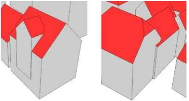
The fourth step of the global half-space adjustment produces among others the following effects. It eliminates misalignments between adjacent building components so that the two adjacent gable roofs in Figure 6 share afterwards the same façade on each side. In addition to that it eliminates undesired extrusions and intrusions in a building façade. These are especially produced by roof structure components like dormers as shown in Figure 9.
Figure 9. These extrusions in the building façades can be automatically eliminated by the global half-space adjustment.
5. FEATURE DECOMPOSITION
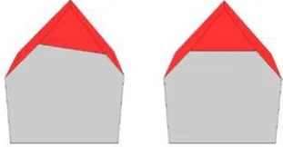
As described in (Kada and Wichmann, 2013) the modeling of buildings using Boolean intersections of planar half-spaces can only produce convex buildings. Therefore, the modeling of a concave building is usually accomplished by partitioning the building into convex components, modeling each component separately, and finally uniting them by a Boolean union operation. According to this procedure a gable roof building with an intrusion has to be partitioned as shown on the left side of Figure 10. In particular the ridge feature and each of its two segments have to be split into three parts. The initial half-spaces of these parts often become unstable due to their small number of supporting points. Thus roof parts of the same segment are sometimes modeled for example with different slopes even after the half-space adjustment steps have been performed.
Figure 10. Two approaches to model a gable roof with an intrusion.
In order to avoid such kind of anomalies we model gable roof buildings first without all intrusions and remove them afterwards by a Boolean difference as shown on the right side of Figure 10. E.g. we allow a feature like the eave to decompose itself so that an intrusion part can have a vertical half-space parallel to the original vertical half-space of the eave. The intrusion parts are determined in the new feature decomposition part of the feature recognition step as follows:
1. Calculate for all alpha-shape points of a ridge segment their perpendicular distance to the ridge and sort them accordingly.
2. Find all clusters containing a number of points greater than a predefined threshold.
3. Each of these clusters – except the minimum and maximum cluster – is partitioned into a minimal number of subsets such that the consecutive distance of any two neighboring points in a subset does not exceed a predefined threshold.
Each subset of points determined in this way defines the length and the position of an intrusion. It is interesting to note that the building outline without all intrusions is given by the maximum cluster of step two.
The feature decomposition part in the feature recognition step is carried out before the half-space adjustment step. Therefore, some half-space adjustments can be performed for each feature part separately and other adjustments like the slope and orientation adjustment in one step for the whole feature.
6. RESULTS
Using the local and global half-space adjustment rules introduced in this paper we have tested the fully automatic feature-driven building reconstruction approach on a part of the Vaihingen test data set provided by the German Society for Photogrammetry, Remote Sensing and Geoinformation (DGPF) (Cramer, 2010). As shown in Figure 11 the building models constructed have very accurate details and are also pleasing to the human eye.
Figure 11. Building models reconstructed in accordance with the rules described in this paper.
Buildings consisting of several components are reconstructed with no unwanted in- or extrusions as shown in Figure 12. Therefore, in our models adjacent building components share the same façade whenever only one façade is expected to be actually present. Also, different components are modeled in such a way that they have common low-level features like ridge, eave and gable end wherever possible. It is interesting to note that the first and the last roof of the right building in Figure 12 has on one side the same slope and the same eave height.
Figure 12. Reconstructed buildings consisting of adjacent gable roofs and wall dormers.
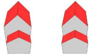
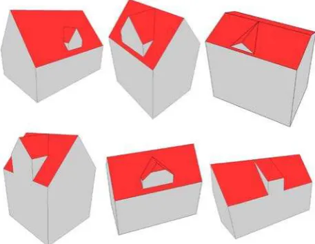
A difficult challenge for a fully automatic reconstruction of building models is usually the reconstruction of dormers and other small building components which belong to other components. Many reconstruction approaches do not consider the interrelationships between such small components and other components. They reconstruct components separately and individually whereas our presented half-space adjustment takes these interrelationships into account. Figure 13 shows some different roof dormer types obtained as a result of our method. The global adjustment leads wherever appropriate to parallelism or co-planarity of a façade of a component and the dormer gable end on its roof, orthogonal ridges, and ridges of equal height. One result of the combination of our local and global half-space adjustment is that dormer hip ends and the roof plane on which they are lying have likely the same x-y orientation.
Figure 13. Reconstructed buildings with different roof dormer types (gabled, eyebrow, partial hipped, and shed).
7. CONCLUSION
In this paper, we improve the accuracy and the shape of building models by using several new regularization rules. These rules take into account advanced building knowledge about local and global building regularities, symmetries, co-planarity, parallelisms and orthogonality. By defining them directly on half-spaces we are able to adjust more than one building feature at the same time without considering the interdependencies of building features. Therefore, our presented local and global half-space adjustments are also suitable for the building reconstruction of large urban areas. In addition to that we have shown how buildings with a concave outline caused by intrusions can be reconstructed by half-space modeling without partitioning them into smaller convex building parts.
ACKNOWLEDGEMENTS
The Vaihingen data set was provided by the German Society for Photogrammetry, Remote Sensing and Geoinformation (DGPF) (Cramer, 2010).
REFERENCES
Alharthy, A., Bethel, J., 2004. Detailed building reconstruction from airborne laser data using a moving surface method. In: The International Archives of Photogrammetry, Remote Sensing and Spatial Information Sciences, 35(B3), pp. 213-218.
Brenner, C., 2010. Building extraction. In: George Vosselman, Hans-Gerd Maas (eds.) Airborne and Terrestrial Laser Scan-ning, Whittles Publishing, pp. 169-212.
Cramer, M., 2010. The DGPF-test on digital aerial camera evaluation – overview and test design. In: Photogrammetrie – Fernerkundung – Geoinformation, 2010(2), pp. 73-82.
Foley, J., van Dam, A., Feiner, S., Hughes, J., 1990. Computer Graphics: Principles and Practice (2nd ed.), Addison-Wesley, Reading, Massachusetts.
Gan, G., Ma, C., Wu, J., 2007. Data Clustering: Theory, Algorithms, and Applications, Society for Industrial and Applied Mathematics, Philadelphia, Pennsylvania.
Haala, N., Kada, M., 2010. An update on automatic 3D building reconstruction. In: ISPRS Journal of Photogrammetry and Remote Sensing, 65(6), pp. 570-580.
Kada, M., Wichmann, A., 2012. Sub-surface growing and boundary generalization for 3D building reconstruction. In: The International Annals of Photogrammetry, Remote Sensing and Spatial Information Sciences, 1(3), pp. 233-238.
Kada, M., Wichmann, A., 2013. Feature-driven 3D building modeling using planar halfspaces. In: The International Annals of Photogrammetry, Remote Sensing and Spatial Information Sciences, 2(3/W3), pp. 37-42.
Kazhdan, M., Funkhouser, T., Rusinkiewicz, S., 2004. Symmetry descriptors and 3D shape matching. In: Proceedings of the Eurographics/ACM SIGGRAPH Symposium on Geometry Processing, 2004, pp. 115-123.
Li, Y., Wu, X., Chrysanthou, Y., Sharf, A., Cohen-Or, D., Mitra, N. J., 2011. GlobFit: Consistently fitting primitives by discovering global relations. In: ACM Transactions on Graphics, 30(4), pp. 52:1-52:12.
Maas, H.-G., Vosselman, G., 1999. Two algorithms for extracting building models from raw laser altimetry data. In: ISPRS Journal of Photogrammetry and Remote Sensing, 54(2-3), pp. 153-163.
Mäntylä, M., 1988. An Introduction to Solid Modeling. Computer Science Press, Rockville, Maryland.
Neidhart, H., Sester, M., 2008. Extraction of building ground plans from LIDAR data. In: The International Archives of Photogrammetry, Remote Sensing and Spatial Information Sciences, 37(B2), pp. 405-410.
Oda, K., Takano, T., Doihara, T., Shibasaki, R., 2004. Automatic building extraction and 3-D city modeling from LIDAR data based on Hough transformation. In: The International Archives of Photogrammetry, Remote Sensing and Spatial Information Sciences, 35(B3), pp. 277-280.
Overby, J., Bodum, L., Kjems, E., Ilsøe, P. M. (2004). Automatic 3D building reconstruction from airborne laser scanning and cadastral data using Hough transform. In: The International Archives of Photogrammetry, Remote Sensing and Spatial Information Sciences, 35(B3), pp. 296-301.
Rosen, J., 1975. Symmetry Discovered: Concepts and Applications in Nature and Science. Cambridge University Press, Cambridge, United Kingdom.
Rottensteiner, F., 2003. Automatic generation of high-quality building models from LIDAR data. In: Computer Graphics and Applications, 23(6), pp. 42-50.
Rottensteiner, F., Trinder, J., Clode, S., Kubik, K., 2005. Automated delineation of roof planes from LIDAR data. In: The International Archives of Photogrammetry, Remote Sensing and Spatial Information Sciences, 36(3/W19), pp. 221–226.
Rottensteiner, F., Sohn, G., Jung, J., Gerke, M., Baillard, C., Benitez, S., Breitkopf, U., 2012. The ISPRS benchmark on urban object classification and 3D building reconstruction. In: The International Annals of Photogrammetry, Remote Sensing and Spatial Information Sciences, 1(3), pp. 293-298.
Sampath A., Shan, J., 2007. Building boundary tracing and regularization from airborne LIDAR point clouds. In: Photogrammetric Engineering and Remote Sensing, 73(7), pp. 805-812.
Tarsha-Kurdi, F., Landes, T., Grussenmeyer, P., Koehl, M., 2007. Model-driven and data-driven approaches using LIDAR data: Analysis and comparison. In: The International Archives of Photogrammetry, Remote Sensing and Spatial Information Sciences, 36(3/W49A), pp. 87–92.
Tarsha-Kurdi, F., Landes, T., Grussenmeyer, P., 2008. Extended RANSAC algorithm for automatic detection of building roof planes from LIDAR data. In: The Photogrammetric Journal of Finland, 21(1), pp. 97-109.
Thrun, S.,Wegbreit, B., 2005. Shape from symmetry. In: Proceedings of the International Conference on Computer Vision, 2005, pp. 1824-1831.
Zhou, Q.-Y., Neumann, U., 2012. 2.5D building modeling by discovering global regularities. In: Conference on Computer Vision and Pattern Recognition, 2012, pp. 326-333.