SENSOR SIMULATION BASED HYPERSPECTRAL IMAGE ENHANCEMENT WITH
MINIMAL SPECTRAL DISTORTION
A. Khandelwala,∗, K. S. Rajanb
a
Dept. of Computer Science and Engineering, University of Minnesota, 200 Union Street SE, Minneapolis, USA - [email protected] bLab for Spatial Informatics, International Institute of Information Technology, Gachibowli, Hyderabad 500032, India - [email protected]
KEY WORDS:Hyperspectral Image Fusion, Spectral Response Functions, Spectral Distortion, Sensor Simulation, Vector Decompo-sition
ABSTRACT:
In the recent past, remotely sensed data with high spectral resolution has been made available and has been explored for various agri-cultural and geological applications. While these spectral signatures of the objects of interest provide important clues, the relatively poor spatial resolution of these hyperspectral images limits their utility and performance. In this context, hyperspectral image enhance-ment using multispectral data has been actively pursued to improve spatial resolution of such imageries and thus enhancing its use for classification and composition analysis in various applications. But, this also poses a challenge in terms of managing the trade-off between improved spatial detail and the distortion of spectral signatures in these fused outcomes. This paper proposes a strategy of using vector decomposition, as a model to transfer the spatial detail from relatively higher resolution data, in association with sensor simulation to generate a fused hyperspectral image while preserving the inter band spectral variability. The results of this approach demonstrates that the spectral separation between classes has been better captured and thus helped improve classification accuracies over mixed pixels of the original low resolution hyperspectral data. In addition, the quantitative analysis using a rank-correlation metric shows the appropriateness of the proposed method over the other known approaches with regard to preserving the spectral signatures.
1. INTRODUCTION
Hyperspectral imaging or imaging spectroscopy has gain consid-erable attention in remote sensing community due to its utility in various scientific domains. It has been successfully used in is-sues related to atmosphere such as water vapour (Schlpfer et al., 1998), cloud properties and aerosols (Gao et al., 2002); issues related to eclogoy such as chlorophyll content (Zarco-Tejada et al., 2001), leaf water content and pigments identification (Cheng et al., 2006); issues related to geology such as mineral detec-tion (Hunt, 1977); issues related to commerce such as agriculture (Haboudane et al., 2004) and forest production.
The detailed pixel spectrum available through hyperspectral im-ages provide much more information about a surface than is avail-able in a traditional multispectral pixel spectrum. By exploiting these fine spectral differences between various natural and man-made materials of interest, hyperspectral data can support im-proved detection and classification capabilities relative to panchro-matic and multispectral remote sensors (Lee, 2004) (Schlerf et al., 2005) (Adam et al., 2010) (Govender et al., 2007) (Xu and Gong, 2007).
Though hyperspectral images contain high spectral information, they usually have low spatial resolution due to fundamental trade-off between spatial resolution, spectral resolution, and radiomet-ric sensitivity in the design of electro-optical sensor systems. Thus, generally multispectral data sets have low spectral resolution but high spatial resolution. On the other hand, hyperspectral datasets have low spatial resolution but high spectral resolution. This coarse resolution results in pixels consisting of signals from more than one material. Such pixels are called mixed pixels. This phe-nomenon reduces accuracy of classification and other tasks (Villa et al., 2011b) (Villa et al., 2011a).
With the advent of numerous new sensors of varying specifica-tions, multi-source data analysis has gained considerable
atten-∗Corresponding author.
tion. In the context of hyperspectral data, Hyperspectral Image Enhancement using multispectral data has gained considerable attention in the very recent past. Multi-sensor image enhance-ment of hyperspectral data has been viewed with many perspec-tives and thus a variety of approaches have been proposed. Algo-rithms for pansharpening of multispectral data such as CN sharp-ening (Vrabel, 1996), PCA based sharpsharp-ening (Chavez, 1991), Wavelets based fusion (Amolins et al., 2007) have been extended for hyperspectral image enhancement. Component substitution based extensions such as PCA based sharpening suffer from the fact that information in the lower components which might be critical in classification and detection may be discarded and re-placed with the inherent bias that exist due to band redundancy. Frequency based methods such as Wavelets have the limitation that they are computationally more expensive, requires appro-priate values of the parameters and in general does not preserve spectral characteristics of small but significant objects in the im-age. Various methods (Gross and Schott, 1998) using linear mix-ing models have been proposed to obtain sub pixel compositions which are then distributed spatially under spatial autocorrelation constraints. The issue with these algorithms is that they do not have robust ways of determining spatial distribution of pixel com-positions. Recently, methods incorporating Bayesian framework (Eismann and Hardie, 2005) (Zhang et al., 2008) have been pro-posed that model the enhancement process in a generative model and achieve enhanced image as maximum likelihood estimate of the model. The challenge with these methods is that they make various assumptions on distribution of data and require certain correlations to exist in data for good performance.
inap-Band Number Spectral Range of List of band numbers of ALI ALI bands (inµm) from HYPERION
Band 3 0.45 - 0.515 11-16
Band 4 0.52 - 0.60 18-25
Band 5 0.63 - 0.69 28-33
Band 6 0.77 - 0.80 42-45
Band 9 1.55 - 1.75 141-160
Band 10 2.08 - 2.35 193-219
Table 1: Set of hyperspectral bands corresponding to each multi-spectral band
propriate for image processing tasks such as classification, object detection etc.
Here, we propose a new approach,Hyperspectral Image Enhance-ment UsingSensorSimulation andVectorDecomposition (HySSVD) for improving spatial resolution of hyperspectral data using high spatial resolution multi-spectral data. This paper aims at explor-ing how well enhanced images from different algorithms mimic the true or desired spectral variability in the fused hyperspectral image. Through various experiments we show that there exits a trade-off between improvement in spatial detail and distortion of spectral signatures.
2. DATA
Hyperspectral data from HYPERION sensor on board EO-1 space-craft has been used for this study. HYPERION provides a high resolution hyperspectral imager capable of resolving 220 spec-tral bands (from 0.4 to 2.5 micrometers) with a 30-meter spatial resolution and provides detailed spectral mapping across all 220 channels with high radiometric accuracy.
For multispectral data, ALI (Advanced Land Imager) sensor on board EO-1 spacecraft has been used. ALI provides Landsat type panchromatic and multispectral bands. These bands have been designed to mimic six Landsat bands with three additional bands covering 0.433-0.453, 0.845-0.890, and 1.20-1.30 micrometers. Multispectral bands are available at 30-meter spatial resolution.
Since hyperspectral bands have very narrow spectral range (10 nm), they are also referred by their center wavelength. Table 1 shows spectral range of multispectral bands that mimic six Land-sat bands together with list of hyperspectral bands whose center wavelength lie in the range of different multispectral bands.
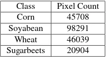
Since, both hyperspectral data and multispectral data are at 30m spatial resolution, hyperspectral data has been down sampled to 120m in this work. Hence the ratio of 4:1 between multispectral data and hyperspectral data has been established. Moreover, in this setting hyperspectral data at 30m can be used as validation data against which output of different algorithms can be com-pared. Here, the hyperspectral data at 30m will be referred to as THS (True Hyperspectral) and hyperspectral data at 120m will be referred as OHS (Original Hyperspectral) which will be enhanced by the algorithms. Multispectral data at 30m will be referred to as OMS. Figure 1 shows RGB composites of datasets used in this study. The algorithms use OHS with OMS to generate the fused hyperspectral image (FHS) at 30m. This fused result would be compared with THS for performance analysis. Figure 1(d) is the class label information for the given area. As we can see, the re-gion contains four major classes namely Corn (green), Soyabean (yellow), Wheat (red) and Sugarbeets (brown) with pixel distri-bution shown in table 2. This image corresponds to an area in Minnesota, USA. The image has been taken on21stJuly, 2012.
Class Pixel Count
Corn 45708
Soyabean 98291
Wheat 46039
Sugarbeets 20904
Table 2: Pixel Count of major classes
(a) (b) (c) (d)
Figure 1: Study Area. (a) True Hyperspectral (THS) image at 30m, (b) Original Multispectral (OMS) image at 30m, (c) Origi-nal Hyperspectral (OHS) image at 120m, (d) Ground Truth map at 30m
The ground truth is available through NASA’s Cropscape website (Han et al., 2012).
In order to properly show the visual quality of various images, magnified view of the part of image enclosed in dotted lines in figure 1(a) will be used. For statistical analysis, the complete image will be used.
3. PROPOSED APPROACH
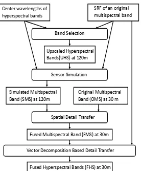
The algorithm presented here, HySSVD has three main stages. Figure 2 shows the flowchart of the algorithm. As a preprocessing step, original low resolution hyperspectral data (OHS) is upscaled to the spatial resolution of original multispectral data (OMS). The upscaled data will be referred as UHS. In the first stage, simu-lated multispectral (SMS) bands are generated using UHS bands and Spectral Response Functions (SRF) of OMS bands. In the second stage, each SMS band is enhanced using its correspond-ing OMS band to generate fused multispectral (FMS) bands. In third stage, Fused Hyperspectral (FHS) bands are computed by inverse transformation using vector decomposition. Following subsections explain each stage in detail.
3.1 Generating Simulated Multispectral (SMS) bands
Center wavelengths of hyperspectral bands
SRF of an original multispectral band
Band Selection
Upscaled Hyperspectral Bands(UHS) at 120m
Sensor Simulation
Simulated Multispectral Band (SMS) at 120m
Original Multispectral Band (OMS) at 30 m
Spatial Detail Transfer
Fused Multispectral Band (FMS) at 30m
Vector Decomposition Based Detail Transfer
Fused Hyperspectral Bands (FHS) at 30m
Figure 2: Flowchart of the Algorithm
1500 1550 1600 1650 1700 1750 1800 0
0.2 0.4 0.6 0.8 1
Wavelength
SRF Value
Figure 3: Spectral response function of band 9 of ALI
to detect. In other words, all the wavelengths that a sensor is able to detect contributes to its value. The weight of the contribution of a particular wavelength is determined by the SRF value at that wavelength. Ideally, to simulate a multispectral band, we need light from all wavelengths within the SRF of that band. But this level of spectral detail is not available in real sensors. Hyperspec-tral sensors are the closest approximation for the data that can be used for simulating a sensor with wide SRF. As mentioned be-fore, SRFs of hyperspectral bands are generally referred by their center wavelengths as they are very narrow. Figure 3 shows these center wavelengths as vertical red lines. The hyperspectral bands that contribute in simulation of a multispectral band are the ones which have their center wavelength within the spectral range of the multispectral band. Table 1 shows the set of hyperspectral bands selected for each multispectral band.
Many methods exist for simulating multispectral data with de-sired wide-band SRFs. Most methods synthesize a multispectral band by a weighted sum of hyperspectral bands, and they are dif-ferent in their ways in determining the weighting factors. Some methods directly convolve the multispectral filter functions to the hyperspectral data (Green and Shimada, 1997), which is equiva-lent to using the values of the multispectral SRF as the weighting factors. Some have used the integral of the product of the hyper-spectral and multihyper-spectral SRFs as the weight (Barry et al., 2002). Few have calculated the weights by finding the least square ap-proximation of a multispectral SRF by a linear combination of the hyperspectral SRFs ( Slawomir Blonksi, Gerald Blonksi, Jeffrey Blonksi, Robert Ryan, Greg Terrie, Vicki Zanoni, 2001). Bowels (Bowles et al., 1996) used a spectral binning technique to get syn-thetic image cubes with exponentially decreasing spectral resolu-tion, where the equivalent weighting factors are binary numbers.
The algorithm presented here has adopted the method described
in (Green and Shimada, 1997). Firstly, all OHS bands are up-scaled to the spatial resolution of the given OMS data to get UHS. Ifmis the number of bands falling in the range of the multispec-tral bandk(OM Sk), then letW~kbe themdimensional weight
vector calculated using spectral response function of the multi-spectral bandk. For a pixel at locationi,j, letU HS~ i,j,kbe the
m dimensional vector containing the intensity values of thosem hyperspectral bands corresponding to (OM Sk). The simulated
value SMSi,j,kfor the pixeli,jcan be obtained using the
follow-ing equation.
SM Si,j,k=W~kTU HS~ i,j,k (1)
which is the inner product of the two vectors. The vectorW~kTis
computed as
Wki=SRFk(Ci) (2)
where,SRFkis the spectral response function of the
multispec-tral bandkandCiis center wavelength of the hyperspectral band
i.
The reason for creating simulated multispectral bands is two-fold. First, since high spatial detail is available at multispectral reso-lution, transferring spatial detail at multispectral level would be more effective than transferring spatial detail from a multispectral band to a hyperspectral band directly. Second, this will ensure that the algorithm is not enhancing a hyperspectral band whose spectral information is not part of a multispectral band in ques-tion. The drawback of this approach is that some hyperspectral bands will not be enhanced. But other approaches will also cause spectral distortion in these bands as multispectral data does not contain information about these bands.
3.2 Generating Fused Multispectral Bands
After stage 1, SMS bands are obtained. These bands have spa-tial resolution same as that of OMS bands but have poor detail as compared to OMS bands because SMS bands are simulated using upscaled hyperspectral bands. In this step, spatial detail from an OMS band is transferred to its corresponding SMS band. This step can be seen as sharpening of a grayscale image using an-other grayscale image. One relevant concern here can be that why there is a need to transfer detail and create a fused multispectral band. Since, theoretically an SMS band is just low spatial reso-lution version of its corresponding OMS band, then OMS band itself can be treated as the fused high spatial resolution version of SMS bands. But in many real situations multispectral data and hyperspectral data can be from different dates. Because of differ-ent atmospheric conditions and other factors, an OMS can not be taken as a direct enhanced version of its SMS band. Hence, we need methods that can transfer only spatial detail while not dis-torting the spectral properties of the SMS band. Many methods exist to do this operation. In this paper Smoothing Filter Based Intensity Modulation (SFIM) algorithm has been adopted (Liu, 2000). SFIM can be represented as
F M Si,j,k= SM Si,j,k
∗OM Si,j,k
OM Si,j,k
(3)
where, OM Si,j,k, SM Si,j,k and F M Si,j,k are original
mul-tispectral value, simulated mulmul-tispectral value and fused multi-spectral value respectively at a pixel i,j for the band k.OM Si,j,k
is the mean value calculated by using an averaging filter for a neighborhood equivalent in size to the spatial resolution of the low-resolution data. Similarly this operation can be applied to enhance each SMS band leading to the calculation of the corre-sponding FMS band.
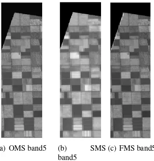
(a) OMS band5 (b) SMS band5
(c) FMS band5
Figure 4: Performance of the Stage 2 spatial detail transfer
dotted lines in figure 1(a) due to space constraints. Figure 4(a) shows band 5 from original multispectral data (OM S5), while
Figure 4(b) shows simulated multispectral band 5 (SM S5)
cor-responding to band 5 of ALI data. Figure 4(c) shows the fused result for band 5 (F M S5). It is clearly evident that features have
become sharper in the fused result. Now this detail has to be transferred to each hyperspectral band that contributed in simula-tion of this band.
3.3 Generating Fused Hyperspectral (FHS) Bands Using Vec-tor Decomposition Method
The previous stage generates FMS bands. The spatial detail from FMS bands has to be transferred into hyperspectral bands. Here, we explain the process of detail transfer at this stage. Expanding equation 1, we have
w1uhs1+w2uhs2+...wm−1uhsm−1+wmuhsm=SM Si,j,k
(4) wherewi anduhsi are elements of vectorsW~k andU HS~ i,j,k
respectively. This is an equation of am dimensional hyperplane on which we know a point,U HS~ i,j,k. This plane will be referred
asPSM S. Also, say normal of this plane isnˆ. SayF HS~ i,j,k
be the m dimensional vector representing fused hyperspectral value for themselected bands of multispectral bandk. Fused multispectral (FMS) data can alternatively be estimated using the sensor simulation strategy from section (3.1).
w1f1+w2f2+...wm−1fm−1+wmfm=F M Si,j,k (5)
wherewiandfiare elements of vectorsW~kandF HS~ i,j,k
re-spectively. Again this is an equation of anm dimensional hy-perplane on which we wish to estimate the pointF HS~ i,j,k. This
plane will be referred asPF M S. Equations 4 and 5 represent two
parallel hyperplanes which are separated by a distancedequal to the difference between the simulated and fused multispectral values at that pixel (F M S~ i,j,k-SM S~ i,j,k).
Since, we aim to achieve enhanced spectra with least spectral distortion, we estimate pointF HS~ i,j,kas a point on the plane
PF M Swhich is closest to the pointU HS~ i,j,kon the planePSM S.
Hence, this point is the intersection of the planePF M Sand the
line perpendicular to planePSM Sand passing through point
~
U HSi,j,k. Figure 5 illustrates the method of estimation using
two dimensions.
The two axes represent two bands of hyperspectral data corre-sponding to a multispectral band. Say,xandyare the values in these bands for a pixel,dis the difference between the simulated
Figure 5: Geometric interpretation of Vector decomposition based detail transfer
multispectral value and the fused multispectral value at that pixel. P1is the plane that represents equation 4 andP2is the plane that represents the equation 5. Here (x,y) can be understood as the components of vectorU HS~ i,j,kand (x+dcosα,y+dsinα)
can be understood as the components ofF HS~ i,j,k.
4. RESULTS AND DISCUSSION
In order to compare the performance of HySSVD with exist-ing work, Principal Component Analysis based technique (PCA) (Tsai et al., 2007) has been implemented for comparison.
PCA first takes the principal component transform of the input low spatial resolution hyperspectral bands corresponding to a given multispectral band. Then first principal component is replaced by the high spatial resolution multispectral band. Then an inverse transform on this matrix returns a high spatial and spectral reso-lution hyperspectral bands.
These methods have been compared qualitatively and quantita-tively. Qualitative analysis has been done by visual inspection of different fused images. For quantitative analysis, classification accuracy on two major classes has been observed. Another met-ric, Kendall Tau rank correlation has been used to measure the spectral signature preservation of different algorithms.
4.1 Qualitative Analysis
In order to see the impact of various algorithms on visual quality of the images, here we show a part of the image.
From visual inspection, we can see that HySSVD has slightly improved the spatial details in the image. HySSVD has slightly sharpened the patch boundaries. But fused image from PCA has much better spatial detail than fused image from HySSVD. So, for visual analysis of RGB composites, PCA based fused image is more suitable among the two algorithms.
4.2 Quantitative Analysis
(a) FHS image from HySSVD
(b) FHS image from PCA
(c) THS image (d) OHS im-age
Figure 6: Magnified view of the selected part of the Study Area
Image Type Soyabean Wheat Overall
OHS 76.45 75.27 76.10
THS 92.61 92.56 92.60
FHS-HySSVD 88.85 89.40 89.02
FHS-PCA 92.06 91.82 91.99
Table 3: Classification Performance on mixed pixels for different image types
Here, we aim to demonstrate that classification results after fu-sion are better than without fufu-sion and compare different algo-rithm based on their classification accuracy. In order to make the evaluation setup less complex, we will consider only the bi-nary classification case. We use bibi-nary Decision Tree to classify the given image into two classes namely Wheat and Soybean. 500 pixels for each class were randomly selected for learning the model. Table 3 shows the overall accuracy and class based ac-curacy for different types of images only on mixed pixels as we want to evaluate algorithms for their ability to improve spatial de-tail of mixed pixels. As explained before, mixed pixels contain spectral combination from multiple land cover types. Since OHS is at 120 meters, each OHS pixel contains 16 THS pixels. So, if it is assumed that pixels at 30 meters are pure, then we can de-fine mixed pixels for OHS. Specifically, any OHS pixel contains THS pixels belonging to more than one land cover type then that pixel is considered as mixed pixel. Since, we are evaluating the results at THS resolution, we considered only those pixels which are part of mixed pixels at OHS resolution.There are 10223 pixel of Soyabean class which are part of any mixed pixel. Similarly, we have 4559 Wheat pixel that are part of any mixed pixel. Accu-racy values are average accuAccu-racy values from 1000 random runs.
Firstly, we can see that from Table 3 that THS has highest class based and overall accuracy. This matches our expectation be-cause THS is itself the high spatial and spectral resolution data that different methods are trying to estimate. HySSVD shows improvement in classification accuracy over OHS. This demon-strates that HySSVD has been able to improve the quality of the input image for image processing tasks such as classification. When compared with the baseline algorithm, PCA appear to do better than HySSVD.
We have observed that fusion methods have lead to improvement in discriminative ability of the data. It is important to note that classification performance depends on the classification task at hand. If the land cover classes are very easy to separate then small distortions in spectral signatures will not impact classifi-cation performance. But for various appliclassifi-cations that use hyper-spectral data, preserving subtle features of the hyper-spectral signature
0 20 40 60 80
0 1000 2000 3000 4000
Pixel Value
Bands Wheat Soyabean
Figure 7: Spectral Signatures of class Soyabean and Wheat
Method Soyabean Wheat Overall
FHS-PCA 0.90 0.68 0.83
FHS-HySSVD 0.90 0.78 0.86
OHS 0.90 0.76 0.86
Table 4: Class wise Rank Correlation values for different meth-ods on mixed pixels
of a land cover class is essential. Hence, improvement in clas-sification should not be the only measure for evaluating spectral fidelity. Figure 7 shows the spectral signature of Wheat and Soy-abean. Vertical lines divides the signature into six sections, each corresponding to a multispectral band. As we can see from the figure, both spectral signatures have subtle features(local mini-mas and maximini-mas) that might be of interest in some applications. Hence, it is important to preserve these features in the fused prod-uct. Hence it is important that different algorithms maintain the relative ordering of values in spectral signatures and hence pre-serving these subtle features of the spectral signatures. Rank correlation measures the consistency between two given order-ings. In our case, we want to measure whether spectral signatures from HySSVD are more consistent with true spectral signatures or spectral signatures from PCA are more consistent. Here we have used Kendall Tau rank correlation measure. Kendall Tau correlation is defined as
-KT=
Pn−1
i=1 Pn
j=i+1sign((Bi−Bj)(Ii−Ij))
Pn−1
i=1 Pn
j=i+11
(6)
where, Bis the reference series of lengthnandI is the input series of lengthn. In words, KT measure the difference between the number of concordant pairs and discordant pairs normalized by total number of pairs. A pair of indices in the series are con-sidered concordant if both reference and input series increase or decrease together from one index to other. Otherwise, the pair is considered discordant.
Table 4 shows class wise and overall rank correlation values on mixed pixels for different algorithms. From above table, we can see that HySSVD has done a good job of preserving relative or-dering of values in the spectrum. For class Soyabean, HySSVD has not shown any improvement but it has notably improved con-sistency for pixels of class Wheat. When compared with the base-line algorithm, PCA perform poorly than HySSVD. In order to understand these results in more detail, we plot the scatter plot of Kendall Tau value for different pairs of data images as shown in figure 8 and 9. In order to reduce number of plots, we have compared HySSVD with only PCA.
0 0.2 0.4 0.6 0.8 1
Figure 8: Scatter plot of Kendall Tau values for class Soyabean
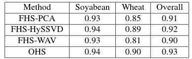
Method Soyabean Wheat Overall
FHS-PCA 0.93 0.85 0.91
FHS-HySSVD 0.94 0.89 0.92
FHS-WAV 0.93 0.81 0.90
OHS 0.94 0.90 0.93
Table 5: Class wise Rank Correlation values for different meth-ods on pure pixels
PCA has more variance than HySSVD. This shows that PCA de-viates more from the original signature and has more propensity for spectral distortion than HySSVD. For class wheat as shown in figure 9, HySSVD is performing better than PCA. At the same time, HySSVD also shows slight improvement over LR. On the other hand, PCA is worse than the original data itself. This tells us that PCA is more aggressive while doing enhancement and deteriorates the relative spectral properties. For HySSVD we can see that it performs very similar to LR which means that it is more conservative and does not alter the LR spectrum very drastically and hence tends to avoid spectral distortion.
A similar analysis is required on pure pixels to ensure that the algorithms are not introducing unwanted characteristics into the signatures that do not need enhancement. Table 5 shows the per-formance on pure pixels.
Again, we can see that HySSVD has maintained the spectral char-acteristics of pure pixels more effectively than PCA. Figure 10 shows anecdotal example of spectral distortion in pure and mixed pixels. Figure 10(a) shows spectral signature of the first 25 bands of a pure pixel. We can see that the amount of distortion by HySSVD is minimal whereas PCA has introduced slight distor-tion in signature. Figure 10(b) shows spectral signature of the first 25 bands of a mixed pixel. We can see that relatively large distor-tion of signature has happened in PCA based image. Even tough signature from HySSVD is also different from required THS sig-nature but it has less distortion.
5. CONCLUSION
The paper presents a novel way of fusing hyperspectral data and multispectral data to obtain an image with good characteristics
0 0.2 0.4 0.6 0.8 1
Figure 9: Scatter plot of Kendall Tau values for class Wheat
5 10 15 20 25
Figure 10: Example Spectral signatures showing spectral distor-tion
of both. Each stage of the algorithm has many choices of sub techniques. For each stage a very fundamental technique has been chosen as a proof of concept, in order to make the idea less complex and easy to understand. Like most other algorithms, the performance of the algorithm might decrease at larger resolution differences due to upscaling of the data in the initial stage. Since the algorithm enhances only those hyperspectral bands which lie in wide-band SRF ranges of the multispectral bands, this leaves some of the bands unsharpened. This is the tradeoff that has been made to maintain spectral integrity of the fused output. At the application level, this drawback will not be consequential as the algorithm will give subsets of enhanced data in each region of the electromagnetic spectrum according to the SRFs of the mul-tispectral bands. This will allow correct classification and mate-rial identification capabilities. Comparison with a baseline algo-rithm shows that HySSVD has some potential of improving spa-tial quality while preserving spectral properties. Through eximents we showed that HySSVD has capability to improve per-formance in classification task. By careful analysis of the char-acteristics of the spectral signatures we demonstrated that base-line algorithm does distort spectral properties. The performance of HySSVD is limited due to very conservative choice of vector decomposition which does not alter original low resolution sig-nal drastically but this also prevents HySSVD from introducing spectral distortion.
ACKNOWLEDGEMENTS
We would like to thank NASA for the collection and free distri-bution of data from HYPERION and ALI sensor onboard EO-1 satellite. We also thank NASA Agricultural Statistics Services for providing high quality information land cover information on different crops in USA.
REFERENCES
Slawomir Blonksi, Gerald Blonksi, Jeffrey Blonksi, Robert Ryan, Greg Terrie, Vicki Zanoni, 2001. Synthesis of multispectral bands from hyperspectral data: Validation based on images acquired by aviris, hyperion, ali, and etm+. Technical Report SE-2001-11-00065-SSC, NASA Stennis Space Center.
Adam, E., Mutanga, O. and Rugege, D., 2010. Multispectral and hyperspectral remote sensing for identification and mapping of wetland vegetation: a review. Wetlands Ecology and Manage-ment 18(3), pp. 281–296.
Amolins, K., Zhang, Y. and Dare, P., 2007. Wavelet based im-age fusion techniques an introduction, review and comparison.
Barry, P., Mendenhall, J., Jarecke, P., Folkman, M., Pearlman, J. and Markham, B., 2002. EO-1 HYPERION hyperspectral ag-gregation and comparison with EO-1 advanced land imager and landsat 7 ETM+. 3, pp. 1648–1651 vol.3.
Bowles, J. H., Palmadesso, P. J., Antoniades, J. A., Baumback, M. M., Grossmann, J. M. and Haas, D., 1996. Effect of spec-tral resolution and number of wavelength bands in analysis of a hyperspectral data set using NRL’s orasis algorithm.
Chavez, P., 1991. Comparison of three different methods to merge multiresolution and multispectral data: Landsat TM and SPOT panchromatic. Photogrammetric Engineering and Remote Sensing 57(3), pp. 295–303.
Cheng, Y.-B., Zarco-Tejada, P. J., Riao, D., Rueda, C. A. and Ustin, S. L., 2006. Estimating vegetation water content with hy-perspectral data for different canopy scenarios: Relationships be-tween AVIRIS and MODIS indexes. Remote Sensing of Environ-ment 105(4), pp. 354 – 366.
Eismann, M. and Hardie, R., 2005. Hyperspectral resolution en-hancement using high-resolution multispectral imagery with arbi-trary response functions. Geoscience and Remote Sensing, IEEE Transactions on 43(3), pp. 455–465.
Gao, B.-C., Yang, P., Han, W., Li, R.-R. and Wiscombe, W., 2002. An algorithm using visible and 1.38-µm channels to re-trieve cirrus cloud reflectances from aircraft and satellite data. Geoscience and Remote Sensing, IEEE Transactions on 40(8), pp. 1659–1668.
Govender, M., Chetty, K. and Bulcock, H., 2007. A review of hyperspectral remote sensing and its application in vegetation and water resource studies. Water Sa.
Green, R. O. and Shimada, M., 1997. On-orbit calibration of a multi-spectral satellite sensor using a high altitude airborne imag-ing spectrometer. Advances in Space Research 19(9), pp. 1387 – 1398.
Gross, H. N. and Schott, J. R., 1998. Application of spectral mix-ture analysis and image fusion techniques for image sharpening. Remote Sensing of Environment 63(2), pp. 85 – 94.
Haboudane, D., Miller, J. R., Pattey, E., Zarco-Tejada, P. J. and Strachan, I. B., 2004. Hyperspectral vegetation indices and novel algorithms for predicting green LAI of crop canopies: Modeling and validation in the context of precision agriculture. Remote Sensing of Environment 90(3), pp. 337 – 352.
Han, W., Yang, Z., Di, L. and Mueller, R., 2012. Cropscape: A web service based application for exploring and disseminating us conterminous geospatial cropland data products for decision support. Computers and Electronics in Agriculture 84, pp. 111– 123.
Hunt, G., 1977. Spectral signatures of particulate minerals in the visible and near infrared. GEOPHYSICS 42(3), pp. 501–513.
Lee, K., 2004. Hyperspectral versus multispectral data for esti-mating leaf area index in four different biomes. Remote Sensing of Environment 91(3-4), pp. 508–520.
Liu, J. G., 2000. Smoothing filter-based intensity modulation: A spectral preserve image fusion technique for improving spa-tial details. International Journal of Remote Sensing 21(18), pp. 3461–3472.
Schlerf, M., Atzberger, C. and Hill, J., 2005. Remote sensing of forest biophysical variables using HyMap imaging spectrometer data. Remote Sensing of Environment 95(2), pp. 177 – 194.
Schlpfer, D., Borel, C. C., Keller, J. and Itten, K. I., 1998. Atmo-spheric precorrected differential absorption technique to retrieve columnar water vapor. Remote Sensing of Environment 65(3), pp. 353 – 366.
Teillet, P., Fedosejevs, G., Gauthier, R., O’Neill, N., Thome, K., Biggar, S., Ripley, H. and Meygret, A., 2001. A generalized ap-proach to the vicarious calibration of multiple earth observation sensors using hyperspectral data. Remote Sensing of Environ-ment 77(3), pp. 304 – 327.
Tsai, F., Lin, E. and Yoshino, K., 2007. Spectrally segmented principal component analysis of hyperspectral imagery for map-ping invasive plant species. International Journal of Remote Sensing 28(5), pp. 1023–1039.
Villa, A., Chanussot, J., Benediktsson, J. A. and Jutten, C., 2011a. Unsupervised classification and spectral unmixing for sub-pixel labelling. In: Geoscience and Remote Sensing Sym-posium (IGARSS), 2011 IEEE International, IEEE, pp. 71–74.
Villa, A., Chanussot, J., Benediktsson, J. and Jutten, C., 2011b. Spectral unmixing for the classification of hyperspectral images at a finer spatial resolution. Selected Topics in Signal Processing, IEEE Journal of 5(3), pp. 521–533.
Vrabel, J., 1996. Multispectral imagery band sharpening study. Photogrammetric Engineering and Remote Sensing 62(9), pp. 1075–1083.
Xu, B. and Gong, P., 2007. Land-use/land-cover classification with multispectral and hyperspectral EO-1 data. Photogrammet-ric Engineering & Remote Sensing 73(8), pp. 955–965.
Zarco-Tejada, P., Miller, J., Noland, T., Mohammed, G. and Sampson, P., 2001. Scaling-up and model inversion methods with narrowband optical indices for chlorophyll content estimation in closed forest canopies with hyperspectral data. Geoscience and Remote Sensing, IEEE Transactions on 39(7), pp. 1491–1507.