T H E J O U R N A L O F H U M A N R E S O U R C E S • 47 • 1
Water Supply and Sanitation in the
Philippines
Daniel Bennett
A B S T R A C T
Water supply investments in developing countries may inadvertently worsen sanitation if clean water and sanitation are substitutes. This paper exam-ines the negative correlation between the provision of piped water and household sanitary behavior in Cebu, the Philippines. In a model of household sanitation, a local externality leads to a sanitation complemen-tarity that magnifies the compensatory response. Empirical results are con-sistent with the hypotheses that clean water and sanitation are substitutes and that neighbors’ sanitation levels are complements. In this situation, clean water may have large unintended consequences.
I. Introduction
Diarrhea is a critical threat to public health in the developing world, killing more people each year than either tuberculosis or malaria (WHO 2002). Diarrhea is the symptom of several life-threatening enteric infections that are trans-mitted through contact with excrement or consumption of dirty water. Children, who play in dirty areas and lack acquired immunity, face the greatest risk of diarrheal disease. Policymakers have often relied on water supply improvements to combat this problem. Examples include the expansion of municipal water systems and the construction of local deep wells. However, public health evaluations of these projects
Daniel Bennett is an assistant professor in the Harris School of Public Policy Studies at the University of Chicago. He thanks Nathaniel Baum-Snow, Jillian Berk, Pedro Dal Bo´, Kenneth Chay, Andrew Foster, Alaka Holla, Robert Jacob, Ashley Lester, Christine Moe, Kaivan Munshi, Evelyn Nacario-Castro, Mark Pitt, Olaf Scholze, and Svetla Vitanova for helpful feedback. Anton Dignadice, Connie Gultiano, Rebecca Husayan, Jun Ledres, Ronnell Magalso, Edilberto Paradela, Robert Riethmueller, Ed Walag, and Slava Zayats provided data and contextual information. The data used in this article can be obtained begin-ning June 2012 through May 2015 from Daniel Bennett, 1155 E. 60th Street, Chicago, IL 60637, dmbennett@uchicago.edu.
[Submitted May 2010; accepted February 2011]
are mixed: Clean water seems beneficial in some contexts but ineffective or even harmful in others (Fewtrell et al. 2005).1
The mixed effectiveness of clean water is paradoxical. A simple model of health production predicts that clean water must improve health unless it causes the recip-ient to consume less of another health input. This paper suggests that the substitut-ability of clean water and sanitation may cause water supply improvements to worsen sanitary conditions. Households find it costly to build and maintain latrines, handle waste properly, and remove the waste left by children and livestock. Clean water may induce recipients to shirk in terms of sanitary behavior by reducing the health impact of sanitation. This type of behavioral response is familiar from other contexts, such as the debate over whether automotive safety improvements encourage reckless driving (for example, Peltzman 1975; Keeler 1994).2
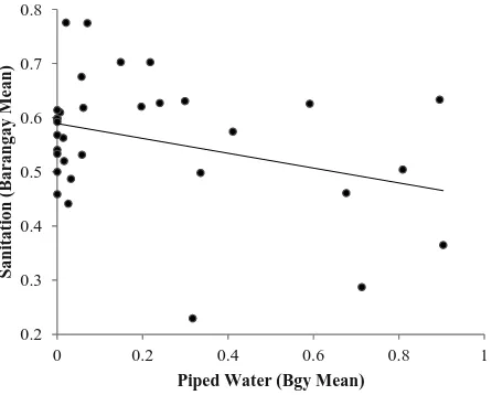
Any compensatory response hinges upon whether clean water and sanitation are complements or substitutes. The relationship between these health inputs is both theoretically ambiguous and empirically unclear. Clean water and sanitation may be substitutes if clean water enables the recipient to endure a dirtier environment with-out sacrificing health. Households also may face a budgetary tradeoff between san-itation and water. On the other hand, these inputs may be health complements if a person must consume both goods to avoid diarrhea. Although the degree of substi-tutability between these inputs may vary by setting, clean water and sanitation are negatively correlated in the present context of Cebu, the Philippines. With greater municipal provision of piped water in Cebu, public defecation has become a severe problem. Neighborhoods with the most piped water tend to exhibit the worst sani-tation.
The complementarity between the sanitation choices of neighbors also mediates any compensatory response to clean water. A sanitation complementarity may arise through either the health production function (if cleanliness by all parties is needed to avoid diarrhea) or through strategic interaction. Sanitation exhibits an obvious externality: Cleanliness by one person protects the entire community. In an effort to internalize the externality, the community may invoke social norms or other strategic mechanisms that lead to a sanitation complementarity (Ostrom 2000; Bandiera, Bar-ankay, and Rasul 2005; Banerjee, Iyer, and Somanathan 2006). According to Akerlof (1980), a social norm leads to a strategic complementarity because compliance strengthens the norm, which begets greater compliance. Other technological and strategic mechanisms also may induce this relationship.
A model in Section II explores this possibility further. A sanitation complemen-tarity can magnify the effect of clean water on sanitation by causing the household to respond to clean water adoption by others in the community. The household’s sanitation response to its own water supply indicates the complementarity or
sub-1. Several economic studies examine sanitation and diarrhea in developing countries. In an evaluation of a deworming program, Kremer and Miguel (2007) and Miguel and Kremer (2004) find positive externalities for school attendance and social learning about the benefits of the program. Kremer et al. (2007) find a marginally significant health impact of spring protection in rural Kenya. Lipscomb and Mobarak (2008) examine the impact of political decentralization on pollution spillovers in Brazil.
stitutability of clean water and sanitation. The sanitation response to the water supply of others reflects both this interaction and the degree of sanitation complementarity across neighbors. An extension of the model considers the sanitation and health impacts of soil thickness, which similarly protects the household from unsanitary conditions.
This framework motivates a regression of sanitation or health on the clean-water usage of both the household and the community. I find across various specifications that sanitation is uncorrelated with piped-water usage of the household but is strongly negatively correlated with usage by the community. Health regressions show a neg-ative correlation between diarrhea and piped water for the household but a positive correlation between diarrhea and piped-water prevalence. These results suggest that clean water and sanitation are weak substitutes but that the sanitation choices of neighbors are strong complements. Soil thickness results also support this theory: Thick soil is negatively correlated with both sanitation and health, but the health impact is especially strong for piped households (for whom thick soil does not confer protection).
Section IV considers the possible influence of confounding factors, including unobservable cross-sectional heterogeneity and the endogenous placement of clean water. My empirical strategy is to show robustness using community or household fixed effects or geographic instrumental variables. These approaches, which utilize different sources of variation, lead to similar estimates. As a falsification test, I also show no effect of clean water on school attendance, which is another human capital investment that is an unlikely substitute for clean water.
II. Theoretical Framework
In this section, I construct a general model of clean water and san-itation in order to motivate the empirical results below. The model illustrates how a sanitation externality may create a sanitation complementarity within the community that magnifies the effect of clean water adoption by others. An extension derives predictions for soil thickness, which like clean water, protects the household from pollution.
A. Setup
A community consists of two households, which are indexed by . Household utilityi
is an additively separable function of health,Hi, and other consumption,ci.Health is increasing and concave in clean water,w iⱖ0, and the sanitation of both house-holds, siⱖ0 and sⳮiⱖ0. By inserting sⳮiinto the health production function of household , I explicitly incorporate a sanitation externality.i 3Households, which are
endowed with incomeYi, face positive prices,P⳱
{
ps,pw,pc}
, of sanitation, clean water, and other consumption. Household solves the following utility maximizationiproblem: , follows from this optimization problem. Each best response *
ci(si,sⳮi,wi; P,Yi)
function must comply with the three first order conditions. Through the implicit function theorem, the first order condition for sanitation yields the partial effect of clean water on sanitation:s*/w⳱ⳮH /H . Because the denominator is
neg-i i s wi i s si i
ative (H is concave), the degree of complementarity between wi andsi signs this expression.
As I show below, the complementarity betweensi andsⳮi also affects the sign and magnitude of the response to clean water.si/sⳮiis unconstrained in general, but either of two factors may create a sanitation complementarity. First, the health production function may exhibit a health complementarity betweensiandsⳮiif, for instance,H⳱f(min
[
s,s]
,w,P,Y). In this situation, even a small amount ofcon-i i ⳮi i i
tamination causes a disease outbreak.
The sanitation game among households also may create a strategic complemen-tarity between si andsⳮi. For example, participants in an infinitely repeated pris-oner’s dilemma may achieve cooperation by threatening to defect if others defect, which causes si/sⳮi⬎0 (Shubik 1970, Arce M 1994). Akerlof (1980) describes how a social norm may induce a large strategic complementarity. Compliance with a social norm strengthens the norm, which encourages greater compliance.4 One explanation for the findings below is that clean water has interfered with a social norm of sanitation.
B. Predictions for Water Supply
I proceed to derive comparative statics that form the basis for subsequent empirical tests. These predictions adopt the perspective of Household 1 and treat Household 2 as the “rest of the community.” I assume thatwiandwⳮiare exogenous for the moment but discuss the endogeneity of these variables in Section IIB. I sign the comparative statics under two assumptions: (1) clean water and sanitation are sub-stitutes (si/wi⬍0), and (2) the sanitation levels of neighbors are complements . These assumptions align the model with the empirical results below. (si/sⳮi⬎0)
However, the reader can easily sign these effects differently to explore alternative assumptions. I also make two simplifying assumptions, which render the model’s
predictions approximate. Some comparative statics exhibit infinite feedback between and . However, the expressions below only incorporate a maximum of three
si sⳮi
feedback terms. I also assume that the rest of the community is much larger than the index household, so thats2/s1⬇0.
The total derivative ofs*with respect tow shows the sanitation response to clean
1 1
water usage by the household. The derivative with respect tow2shows the response to clean water usage by the rest of the community.
*
In Equation 3, the response to clean water usage by the household reflects the substitutability of clean water and sanitation. In Equation 4, the sanitation comple-mentarity multiplies the response to usage by others, causing it to exceed the effect of usage by the household ifs1/s2⬎1. The combination of a small compensatory response with a large complementarity leads to the prediction thatds1/dw1⬇0but
.
ds1/dw2⬍⬍0
The total derivative of H*with respect to w shows the health impact of clean
1 1
water usage by the household. The derivative with respect tow2shows the impact of usage by others.
In Equation 5, clean water directly improves health but also induces a decline in sanitation, which worsens health. The net health impact is positive as long as the direct benefit is large or the compensatory response is small. In contrast, clean water usage by others (which does not directly benefit Household 1) unambiguously wors-ens health by reducing sanitation for both households in Equation 6.
C. Predictions for Soil Thickness
piped water to reduce disease risk, the predictions above do not directly cross-apply because soil thickness is constant within the community.
Soil thickness, T, enters the model as another health input: H⳱H(s,s ,w,T). i i ⳮi i Utility maximization leads to best response functions that now depend on T. The total derivatives ofs*andH*with respect toTshow the sanitation and health effects
1 1
of soil thickness. I sign effects under the assumption that soil thickness and sanitation are substitutes(s/T⬍0).5
Equation 7 shows that soil thickness reduces the sanitation of both households. The sanitation complementarity increases the overall effect by incorporating the feedback from Household 2 to Household 1. In Equation 8, the health impact of the sanitation response offsets the direct benefit of thick soil, leading to an ambiguous net effect. To explore the interaction between soil thickness and clean water, suppose for simplicity that households are either piped(w ⳱1) or nonpiped(w ⳱0).6Neither
1 1
the sanitation nor health of piped households responds directly to soil thickness and if . Applying these assumptions to Equation 7
* *
(si/T⳱0 Hi/T⳱0 wi⳱1)
shows that piped water diminishes the sanitation response to soil thickness. For piped households, the sanitation complementarity drives the entire response to soil thick-ness. Therefore, a large sanitation response for piped households is additional evi-dence of a sanitation complementarity. The difference in Equation 7 between non-piped and non-piped households identifies the partial effect of soil thickness,s1/T. A finding thats1/Tis the same for piped and nonpiped households indicates thats1 and T are weak substitutes becauses1/T⬇0. Finally, the assumption that piped households do not directly respond to soil thickness implies that the health impact of soil thickness is unambiguously negative for this group. Piped households do not benefit from thick soil but suffer under the ensuing sanitation decline.
D. The Endogeneity of Piped Water
This subsection illustrates formally the endogeneity of clean water and highlights the threats to identification in the empirical analysis. Comparative statics for clean water adoption with respect to sanitation and health show how these variables may be correlated through mechanisms other than the causal effects above. The discussion
5. Soil thickness is a parameter rather than a choice variable. As a substitute for sanitation, soil thickness reducesHi/si. The model requires that households perceiveHi/si but not that they knowT or its health implications.
focuses on the endogeneity ofw2, which is most central to the potential for a spurious effect of piped water prevalence. Comparative statics in terms of w1 are signed equivalently.
Two modifications of the basic setup allow the model to encompass the primary confounds. The inclusion of a health endowment,i, allows the best response func-tion w* to depend upon an unobservable health shock. Although the interaction
i
betweeniand other health inputs is unrestricted, I assume that it is a substitute for clean water and sanitation in the comparative statics below. Secondly, I define the price of clean water to be an increasing function of sanitation and health: p ⳱
w . This function captures the possibility that policymakers may target
pw(si,sⳮi,i,ⳮi)
clean water to households with poor sanitation or health. With these modifications, the total derivatives ofw* with respect tos and delineate the channels through
2 1 i
which the endogeneity of clean water may cause a spurious correlation with sani-tation and health.
Equation 9 shows that w2and s1 may be negatively correlated because poor sani-tation encourages clean water adoption directly or spurs policymakers to subsidize clean water. Equation 10 shows that the health implication of clean water endoge-neity is ambiguous. A health improvement directly discourages clean water targeting in the first term of the expression. However a health improvement also leads to diminished sanitation, which encourages clean water adoption in the second term of the expression. The first term must dominate to generate a spurious negative cor-relation between piped water prevalence and health.
The endogeneity of clean water introduces several new terms into the soil thick-ness comparative statics in Equations 7 and 8. The direction of spurious correlation between soil thickness and sanitation and health is ambiguous because thick soil both discourages clean water adoption directly, but also worsens sanitation (which encourages clean water adoption). In Section IV, I discuss the empirical approach and argue that the bias arising because of clean water endogeneity is small.
III. Context and Data
democrati-0.0 0.2 0.4 0.6 0.8 1.0
1983 1991 1994 1998 2002 2005
Pi
ped Wat
er
(B
arangay
Mean)
Year
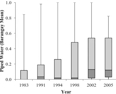
Figure 1
The Distribution of Piped Water Prevalence by Year
cally elected captain leads each barangay and receives municipal funds to maintain public spaces and provide basic health care.
The Metro Cebu Water District (MCWD) delivers chlorinated piped water to around 40 percent of area households. The MCWD obtains water from 110 high-volume deep wells, which are located inland from the city, and stores water in several area reservoirs. Subscribers pay $86 for installation, $2.70 per month for a half-inch connection, and $0.30 per cubic meter of water. This fee schedule subsidizes poor households, and a “community well” program places communal taps in disadvan-taged areas. A household is defined as having piped water if the MCWD is its “usual main source of drinking water.” This definition does not distinguish between actual subscribers and households that obtain piped water from neighbors or community wells. Since its establishment in 1976, the MCWD has gradually expanded its cov-erage of the city. Figure 1, a box-whisker plot of piped water prevalence, shows that the MCWD has expanded service on both the extensive and intensive margins.
As an alternative to the MCWD, households may obtain water from boreholes, dug wells, or artesian springs. These sources are easily accessible because Cebu’s water table lies just a few meters below ground. According to Moe et al. (1991), who analyzed the water quality from various sources in Cebu, these alternatives are generally dirtier than the MCWD supply. In communities near the ocean, seawater intrusion threatens the quality of the groundwater and forces residents to seek alter-native drinking water sources.
This paper relies on data from the Cebu Longitudinal Health and Nutrition Survey (CLHNS), a panel survey of around 3,000 households over 22 years. The sample includes all households that experienced a birth from June 1983-May 1984 in 33 randomly selected barangays. Of the sample population, 74 percent is concentrated in the 17 barangays that are designated as “urban.” Surveyors conducted 12 bi-monthly interviews with each household from 1983 to 1985, and followed up five additional times from 1991 to 2005. By employing a fertility-selected sampling methodology, the CLHNS potentially overrepresents poor households, which are relatively fertile. Adair et al. (1997) explore this issue by comparing the sample of CLHNS mothers to women in the 1980 census. While they find that the sample is not nationally representative, it does represent ever-married women with at least one child in 1980. As a panel survey, the CLHNS captures a sample that is relatively young in early rounds and old in late rounds.
I measure sanitation through a surveyor observation of the amount of excrement near the respondent’s home. In each of six rounds from 1983–2005, the surveyor indicates whether there is: (1) heavy defecation in the area, (2) some defecation in the area, (3) very little excreta visible, or (4) no excreta visible. I collapse this variable into a binary outcome by combining Categories 1 and 2 and Categories 3 and 4. Despite the loss of information, this step facilitates the comparison of esti-mates across OLS, fixed effects, and IV regressions.7Appendix Table A1 demon-strates that key results are robust to variations on this construction. The table also shows results for the absence of garbage, an alternative sanitation measure.
Data on diarrhea are available from the 12 bimonthly surveys, 1983–85. In each interview, the respondent indicates whether the index child, the index mother, or others in the household experienced diarrhea during the previous week. The union of these responses indicates whetheranyonein the household experienced symptoms. I use this measure as the primary diarrhea outcome below, although estimates that isolate the index child give similar results. Since piped water varies only slightly over two years, I collapse the diarrhea reports into a count over 12 intervals. There-fore, diarrhea data are only available as a cross-section from the first round of the survey.
I rely on several observable characteristics to control for heterogeneity across households.Educationis the number of years of schooling attained by the household head. For households with school-aged children,enrollment, andgrade for age in-dicate current human capital investment. I measure the age composition of the house-hold by calculating the percent of the househouse-hold’s members who fall into four age bins: four and younger, 5–10, 11–15, and older than 15. I also calculate the percent of the household’s members who are male.Keeps animalsis an indicator that house-hold keeps animals such as dogs, pigs, and roosters, which are large waste producers.
Toilet/latrineis an indicator that the household has access to a toilet or latrine.
While the CLHNS lacks reliable measures of income or monetary wealth, the durability of the respondent’s house is a close proxy. The survey categorizes houses
0.2 0.3 0.4 0.5 0.6 0.7 0.8
0 0.2 0.4 0.6 0.8 1
Sani
tati
on (B
arangay
Mean)
Piped Water (Bgy Mean)
Figure 2
Piped Water Prevalence and Sanitation
as either: “light,” using nipa or similar materials, “medium,” with a wood or cement foundation but nipa walls or roof, or “strong,” with a wood or cement foundation and a galvanized iron roof. The mean and standard deviation of educationacross other community members measure the barangay’s distribution of socioeconomic status.
The regressions below control directly for population density because this variable obviously confounds the relationship between clean water and sanitation. The first round of the survey measures density in categories ranging from “very low” to “very high,” which I convert into dummies. Subsequent rounds quantify density as the number of houses within 50 meters of the respondent’s home. I divide this variable into five groups to increase its flexibility as a control, although the original definition leads to similar results. To avoid discarding the first survey round, I interact the first-round density variables with a first-round indicator and interact later-round den-sity variables with a later-round indicator. This approach makes it possible to utilize both sets of density variables in parallel.
0 0.5 1 1.5 2 2.5 3
0 0.2 0.4 0.6 0.8 1
Diarrhea Morbi
d
ity (Cases on
12 Intervals)
Piped Water (Bgy Mean)
Figure 3
Piped Water Prevalence and Diarrhea
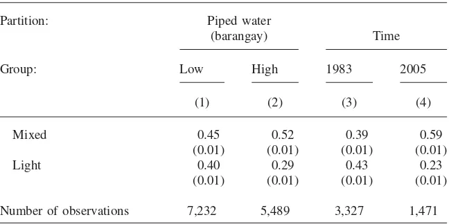
To help interpret these correlations, Table 1 reports the mean and standard error of piped water, sanitation, and several household characteristics. Columns 1 and 2, which split the sample according to mean piped water prevalence (0.306), demon-strate that obvious confounders cannot drive the relationship between clean water and sanitation. Households in high prevalence areas have two additional years of schooling and 26 percent fewer domesticated animals. They also have fewer young children, live in more robust housing, and have greater access to toilets or latrines. These observable characteristics suggest that communities with clean water should exhibit better sanitation and health. Columns 3 and 4 illustrate a similar point by comparing the first and last survey rounds. Piped water prevalence grew by 18 percent from 1983 to 2005. Although trends in household characteristics ostensibly encouraged sanitation, this outcome fell by 8 percent over the period.8
IV. Estimation
This section empirically tests the model’s predictions. If clean water and sanitation are substitutes, then these variables should be negatively correlated. A sanitation complementarity magnifies the sanitation response to clean water usage by others. If clean water and sanitation are weak substitutes but the sanitation levels of neighbors are strong complements, then a regression may only detect the effect
Table 1
Comparisons of Means by Piped Water Prevalence and Time Period
Partition: Piped water
(barangay) Time
Group: Low High 1983 2005
(1) (2) (3) (4)
Piped water 0.05 0.66 0.23 0.40
(0.00) (0.01) (0.01) (0.01)
Sanitation 0.56 0.46 0.66 0.59
(0.01) (0.01) (0.01) (0.01)
Diarrhea 1.88 2.11 1.96 —
(0.04) (0.06) (0.03)
Toilet/latrine 0.59 0.93 0.72 0.83
(0.01) (0.00) (0.01) (0.01)
Keeps animals 0.67 0.41 0.55 0.51
(0.01) (0.01) (0.01) (0.01)
Density 14.9 19.41 — 17.1
(0.10) (0.03) (0.14)
Education
Attainment of head 6.52 8.75 7.37 7.61
(0.04) (0.05) (0.07) (0.10)
Enrollment of children 0.75 0.79 — 0.77
(0.01) (0.01) (0.01)
Grade for age of children 0.53 0.61 0.42 0.63
(0.00) (0.00) (0.01) (0.01)
Percent of household
Age ⬍ 5 0.16 0.12 0.24 0.10
(0.00) (0.00) (0.00) (0.00)
Age 5–10 0.13 0.12 0.10 0.05
(0.00) (0.00) (0.00) (0.00)
Age 11–15 0.14 0.15 0.06 0.09
(0.00) (0.00) (0.00) (0.00)
Age ⬎ 15 0.56 0.62 0.60 0.76
(0.00) (0.00) (0.00) (0.00)
Male 0.50 0.51 0.49 0.51
(0.00) (0.00) (0.00) (0.00)
Home construction (percent)
Strong 0.15 0.20 0.18 0.17
(0.00) (0.01) (0.01) (0.01)
Table 1(continued)
Partition: Piped water
(barangay) Time
Group: Low High 1983 2005
(1) (2) (3) (4)
Mixed 0.45 0.52 0.39 0.59
(0.01) (0.01) (0.01) (0.01)
Light 0.40 0.29 0.43 0.23
(0.01) (0.01) (0.01) (0.01)
Number of observations 7,232 5,489 3,327 1,471
Notes: standard errors appear in parentheses. In Columns 1 and 2, the sample is divided by the mean of piped water prevalence (0.306).
of piped water prevalence. This scenario also leads to countervailing health im-pacts of clean water for the household and for its neighbors.
I regress sanitation and diarrhea on piped water usage by the household and the rest of the community. In the following specifications,i indexes the household, j
indexes the barangay, and tindexes the survey round.
⬘
s ⳱␣Ⳮ␣ w Ⳮ␣w¯ ⳭX ␣Ⳮ⑀
(11) ijt 0 1 ijt 2 jt ijt 3 ijt ⬘
d ⳱Ⳮw Ⳮw¯ ⳭX Ⳮu
(12) ij 0 1 ij 2 j ij 3 ij
is a binary sanitation measure, is an indicator that the household uses MCWD
si wi
piped water, andw¯ is the percent of other sample households in the barangay who use piped water. X is a vector of household and community characteristics. All regressions control for the education of the household head.9All OLS and IV re-gressions, as well as some fixed effects rere-gressions, control for population density as described above. Some specifications also control for the household’s size and its age and gender composition. Standard errors are clustered by barangay and are robust to heteroskedasticity.
Because clean water is allocated nonrandomly, several omitted variables may con-found these estimates. A key concern is that poor sanitation or health may encourage people to adopt clean water. Unobserved heterogeneity in barangay or household
characteristics also could cause a spurious correlation. Urban barangays, many of which are dirty and congested, disproportionately utilize piped water.10
Measurement error inw¯ also could complicate identification. As a sample mean, is subject to classical measurement error through sampling variation in the set of
w¯
households who appear in the survey. With a median of 50 sample households per barangay, sampling variation leads to attenuation of around 2 percent in the coeffi-cient magnitudes below.11The nonrandom selection of the sample also creates non-classical measurement error inw¯ that may cause an ambiguous bias. Respondents, all of whom gave birth during 1983–84, are disproportionately young in early years and old in later years. However, piped water is uncorrelated with age, which reduces the concern that the survey systematically mismeasuresw¯.
My empirical approach addresses these issues by exploiting distinct sources of variation. Either cross-sectional heterogeneity or endogenous water utilization may bias OLS regressions, which rely on both cross-sectional and time-series variation. Fixed effects regressions control for cross-sectional heterogeneity but do not address the endogeneity of clean water. Instrumental variables regressions deal with endog-enous placement through instruments that are not determined by sanitary or health conditions but also may capture undesirable cross-sectional heterogeneity. OLS, fixed effects, and IV approaches yield similar estimates despite their divergent lim-itations. The congruity of the estimates is reassuring because any particular omitted variable would be unlikely to bias these specifications in the same way.
A. OLS and Fixed Effects
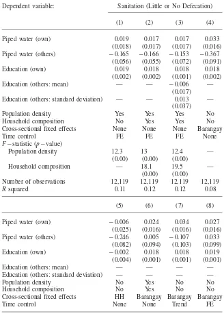
OLS and fixed effects estimates of Equation 11 appear in Table 2. Coefficients represent marginal effects in the linear probability model. Column 1 shows a par-simonious specification that only controls for education and population density. This regression finds no effect ofwiand a negative and significant effect of . An increasew¯
inw¯ of one standard deviation (0.34) is associated with 6 percent worse sanitation. Columns 2 and 3 validate this result using additional controls. Column 2 includes household composition (the household’s size and age and gender distributions) and Column 3 includes the mean and standard deviation of education for others in the community.12
10. Residential sorting may confound the results if households sort based on sanitary preferences. To cause a bias in the observed direction, households that are intrinsically clean mustavoidareas with piped water. Table 1 discounts this possibility by showing that wealthy and educated households do live in areas with piped water.
11. Define observed piped water prevalence as the sum of the true prevalence,w¯*and the sampling error: j
. In a bivariate regression, the ratio of the attenuated coefficient to the true coefficient equals *
w¯⳱w¯ Ⳮe j j j
(Wooldridge 2001, p.75). I gauge the extent of the attenuation bias by inserting proxies
2 2 2
Table 2
Regressions of Sanitation on Water Supply
Dependent variable: Sanitation (Little or No Defecation)
(1) (2) (3) (4)
Piped water (own) 0.019 0.017 0.017 0.033
(0.018) (0.017) (0.017) (0.016) Piped water (others) ⳮ0.165 ⳮ0.166 ⳮ0.153 ⳮ0.367
(0.056) (0.055) (0.072) (0.091)
Education (own) 0.019 0.018 0.018 0.018
(0.002) (0.002) (0.001) (0.002)
Education (others: mean) — — ⳮ0.006 —
(0.017) Education (others: standard deviation) — — 0.013 —
(0.037)
Population density Yes Yes Yes No
Household composition No Yes Yes No
Cross-sectional fixed effects None None None Barangay
Time control FE FE FE None
Fⳮstatistic (pⳮvalue)
Population density 12.3 13 12.4 —
(0.00) (0.00) (0.00)
Household composition — 18.1 19.5 —
(0.00) (0.00)
Number of observations 12,119 12,119 12,119 12,119
Rsquared 0.11 0.12 0.12 0.08
(5) (6) (7) (8)
Piped water (own) ⳮ0.006 0.024 0.034 0.027
(0.025) (0.016) (0.016) (0.016)
Piped water (others) ⳮ0.246 0.005 ⳮ0.107 0.033
(0.082) (0.094) (0.103) (0.099)
Education (own) ⳮ0.002 0.018 0.018 0.019
(0.004) (0.001) (0.001) (0.001)
Education (others: mean) — — — —
Education (others: standard deviation) — — — —
Population density No Yes No No
Household composition No Yes No No
Cross-sectional fixed effects HH Barangay Barangay Barangay
Time control None None Trend FE
Table 2(continued)
Dependent variable: Sanitation (Little or No Defecation)
(5) (6) (7) (8)
Fⳮstatistic (pⳮvalue)
Population density — 19.7 — —
(0.00)
Household composition — 36.4 — —
(0.00)
Number of observations 12,119 12,119 12,119 12,119
R squared 0.33 0.12 0.08 0.14
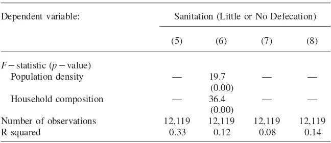
Notes: Standard errors appear in parentheses. Standard errors are clustered by barangay and are robust to heteroskedasticity. Education is the years of schooling of the household head. Population density is a categorical variable in 1983 and a set of bins in subsequent years, as explained in the text. Household composition includes household size, the age distribution across four categories (as defined in the text), and the distribution across genders.
The remainder of Table 2 uses fixed effects to control for time-constant cross-sectional heterogeneity. Column 4 includes barangay fixed effects and Column 5 includes household fixed effects. These estimates are statistically significant and comparable to the OLS results. Unlike OLS or IV specifications, these regressions omit time fixed effects to avoid limiting the extent of time-series variation in sani-tation and piped water. While secular trends could confound these specifications, the robustness of the OLS and IV estimates (which do include time fixed effects) min-imizes this concern. For completeness, Columns 6–8 provide estimates with baran-gay fixed effects as well as additional controls (for density and household compo-sition), a linear time trend, and time fixed effects. Estimates are not robust under these specifications, although the estimate in Column 7 (with a linear time trend) is consistent with the results in Columns 1–5.13 In sum, the fixed effects estimates discount the identification threat from time-constant heterogeneity.
Regressions of diarrhea on water supply based on Specification 12 appear in the Table 3. The table reports estimates for the full sample in Columns 1 and 2, and then divides the sample bywiin Columns 3–6. In each case, one regression controls for education and population density, while another additionally controls for house-hold composition.14Clean water usage by the household is associated with 9 percent less diarrhea in Columns 1 and 2. The net positive health impact of clean water provides further evidence of a small compensatory response to clean water. In
con-13. The barangay fixed effects specification in Column 4 has a lowerR2statistic than the OLS specification in Column 1 because the OLS regression includes population density variables and time fixed effects, which contribute to the explanatory power of the model.
Table 3
Regression of Diarrhea on Water Supply
Dependent variable Diarrhea
Sample Full Nonpiped Piped
(1) (2) (3) (4) (5) (6)
Piped water (own) ⳮ0.174 ⳮ0.177 — — — —
(0.100) (0.109)
Piped water(others) 0.568 0.569 0.760 0.756 0.277 0.278 (0.331) (0.335) (0.469) (0.472) (0.342) (0.325) Education (own) ⳮ0.022 ⳮ0.020 ⳮ0.017 ⳮ0.014 ⳮ0.049 ⳮ0.046
(0.010) (0.010) (0.011) (0.011) (0.012) (0.012) Population density Yes Yes Yes Yes Yes Yes Household composition No Yes No Yes No Yes
Fⳮstatistic (pⳮvalue)
Population density 1.48 1.55 1.43 1.59 34.03 34.78 (0.23) (0.21) (0.25) (0.20) (0.00) (0.00) Household composition — 4.52 — 2.87 — 4.37
(0.01) (0.04) (0.02) Number of observations 3,113 3,113 2,447 2,447 666 666
Rsquared 0.16 0.17 0.16 0.16 0.18 0.18
Notes: Standard errors appear in parentheses. Standard errors are clustered by barangay and are robust to heteroskedasticity. Regressions also control for the number of intervals on which any observation is re-corded.
trast, w¯ has a negative and significant health impact: An increase of one standard deviation (0.27) increases diarrhea by 8 percent. This finding is consistent with a sanitation complementarity, which magnifies the health impact of a sanitation decline by others. Columns 3–6 show that this impact occurs differentially among nonpiped households, whose water supply is less protected from poor sanitation.
B. Instrumental Variables
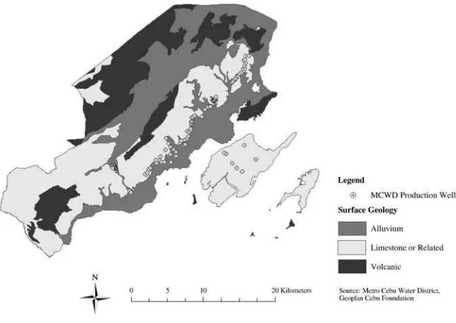
Figure 4
Surface Geology and the Location of Municipal Source Wells in Cebu
illustrates, The MCWD has primarily developed wells along the geological boundary between alluvium and limestone. This region is advantageous for industrial pumping because it avoids both saline intrusion and challenging volcanic geology. Because of the cost of transporting water over land, the MCWD provides less service to barangays that are far from this zone.
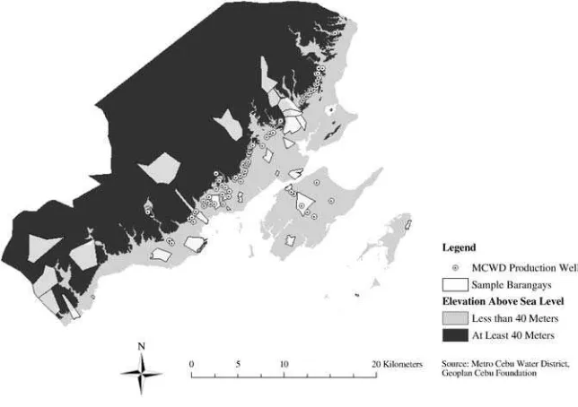
Mountain topography also impedes the provision of piped water. Although it can exploit gravity to move water downhill, the agency must rely on expensive pumps to move water uphill. Barangays located uphill from the extraction zone are unlikely to receive piped water. Because the elevation of this zone is 35–40 meters, a dummy variable for elevations greater than 40 meters serves as another instrument. Figure 5 shows the location of sample barangays relative to this threshold. Near the coast, seawater intrusion threatens the integrity of the local aquifer. Residents with saline groundwater must seek drinking water from either the MCWD or a private vendor. Figure 6 maps the salinity gradient at the water table in 1985 based on MCWD contour maps. Because of the MCWD’s response to this demand, areas with high salinity have greater access to piped water.
Figure 5
Areas Above and Below 40 Meters and the Location of Municipal Source Wells in Cebu
Although they are unlikely to affect sanitation directly, the instruments may be incidentally correlated with unobservable aspects of sanitation. I assess this potential issue by regressing the household characteristics from Table 1 onw¯ as predicted by the instruments. Although the instruments are not balanced on observables, any bias works against the observed results (estimates are available from the author). House-holds with high predictedw¯ have better education and sanitary facilities, as well as fewer young children and domesticated animals. IV estimates for sanitation, which appear in Panel B of Table 4, show a negative and significant effect of w¯. The magnitude ranges fromⳮ0.24 toⳮ0.26, falling between the OLS and fixed effects estimates. A test of overidentifying restrictions evaluates econometrically whether the instruments are correlated with the second-stage error term. With a p-value greater than 0.83, the Hansen J statistic cannot reject the hypothesis that the instru-ments are exogenous. A comparison of Columns 1 and 2 shows that the effect of is insensitive to controlling for household composition. Given the likely
corre-w¯
lation between household composition and other unobservables, this result mitigates the concern over other confounding factors.
C. A Falsification Test Using School Attendance
Figure 6
Groundwater Salinity (Parts Per Million) in Cebu, 1985
human capital investment with common factors such as preferences and socioeco-nomic status. However, recipients of clean water are unlikely to substitute out of education because education, unlike sanitation, does not directly prevent diarrhea. A finding that clean water reduces education suggests that the original result for sanitation arises through a spurious correlation. Conversely, the absence of this find-ing indirectly validates the sanitation results.
Two educational outcomes proxy for the school attendance of children in sample households. School enrollment, which is available in Rounds 3–6, is an indicator of whether each child is currently enrolled in school. Grade for age, which is a noisier measure of attendance, also is available in Round 1. I construct grade for age by dividing the child’s grade attainment by his or her age, subtracting five from the denominator since children begin schooling at age six. Children who enter on time and remain enrolled report a grade for age of 1 in every year, but those who start late or drop out have lower values. I average both attendance outcomes across school-aged (aged 6–16) children in the household.
Table 4
Instrumental Variables Regressions of Sanitation on Water Supply
Second stage dependent variable Sanitation
(1) (2)
Panel A: First Stage
Distance to boundary ⳮ0.041 ⳮ0.041
(0.014) (0.014)
Elevation threshold ⳮ0.199 ⳮ0.198
(0.087) (0.087)
Groundwater salinity 0.002 0.002
(0.001) (0.001)
Panel B: Second Stage
Piped water (others) ⳮ0.244 ⳮ0.259
(0.101) (0.103)
Education (own) 0.021 0.020
(0.003) (0.003)
Population density Yes Yes
Household composition No Yes
Year fixed effects Yes Yes
Fⳮstatistic (pⳮvalue)
Instruments 6.80 6.83
(0.00) (0.00)
Density 57.88 52.4
(0.00) (0.00)
Composition — 91.39
(0.00)
Anderson Rubin statistic 9.12 9.75
(0.03) (0.02)
HansenJstatistic 0.38 0.34
(0.83) (0.84)
Number of observations 12,120 12,120
Rsquared 0.11 0.11
Notes: Standard errors appear in parentheses. Standard errors are clustered by barangay and are robust to heteroskedasticity. The HansenJStatistic and the Anderson-Rubin Statistic are distributed chi squared. The Hansen J Statistic tests whether the instruments are exogenous. The Anderson-Rubin Statistic tests the significance of the endogenous regressor under weak instruments.
result is approximately zero. Overall, these regressions do not replicate the pattern that exists for sanitation.15
Bennett
167
Dependent variable: Enrollment Grade for age
Model OLS FE IV OLS FE IV
(1) (2) (3) (4) (5) (6)
Piped water (own) 0.013 0.022 — 0.010 0.016 —
(0.014) (0.015) (0.008) (0.009)
Piped water (others) ⳮ0.071 0.424 ⳮ0.097 ⳮ0.031 0.380 0.009
(0.050) (0.281) (0.071) (0.019) (0.059) (0.034)
Education (head) 0.014 0.014 0.015 0.012 0.014 0.011
(0.002) (0.001) (0.002) (0.001) (0.001) (0.001)
Population density Yes No Yes Yes No Yes
Household composition Yes No Yes Yes No Yes
Cross-sectional fixed effects None Barangay None None Barangay None
Time control FE None FE FE None FE
Fⳮstatistic (pⳮvalue)
Population density 2.5 — 9.0 4.5 — 13.6
(0.08) (0.06) (0.01) (0.01)
Household composition 5.8 — 31.5 560.8 — 2821.3
(0.00) (0.00) (0.00) (0.00)
HansenJstatistic — — 0.76 — — 0.90
(0.68) (0.64)
Number of observations 5,984 5,984 5,984 7,557 7,557 7,557
R squared 0.06 0.12 0.06 0.39 0.13 0.39
D. Soil Thickness
Like piped water, soil thickness protects the community from poor sanitation. Re-gressions on soil thickness evaluate whether sanitation and health respond to this parallel factor in an expected way. If soil thickness and sanitation are substitutes, then communities with thick soil should exhibit worse sanitation. Equation 7 illus-trates how a sanitation complementarity may magnify the compensatory response to soil thickness.
A comparison of effects for piped and nonpiped households leads to three addi-tional tests. First, the sanitation response by piped households singles out the sani-tation complementarity (the second term in the comparative static) because piped households do not respond directly to soil thickness. Secondly, the differential re-sponse of nonpiped households isolates the direct compensatory rere-sponse (the first term in the comparative static). A similar sanitation effect for piped and nonpiped households indicates that the compensatory response is small. Finally, the health impact of soil thickness in Equation 8, which is ambiguous in general, is clearly negative for piped households. The diarrhea regression for piped households tests this hypothesis.
The CLHNS measures soil thickness through a categorical variable recorded in the first survey round. The possible values, which are uniform within a barangay, are (1) less than 0.3 meters, (2) 0.3 to 1 meters, (3) 1 to 3 meters, and (4) greater than 3 meters. Since soil under one meter thick does not attenuate pathogens sub-stantially, I combine Groups 1 and 2 and regress on two soil thickness categories (with one excluded).16 According to summary statistics by soil thickness category (available from the author), households with thick soil have more schooling, better sanitary facilities, and fewer domesticated animals. Piped water also is positively correlated with soil thickness.
The following specifications evaluate the effect of soil thickness on sanitation and diarrhea.
Effects of the categorical soil thickness measure, j, are measured relative to the group with the thinnest soil, which is excluded.Xis a vector of household charac-teristics that is consistent with earlier regressions.
Regressions of sanitation and diarrhea on soil thickness appear in Table 6. For each outcome, the table distinguishes between piped and nonpiped households, and shows a regression with few and with many controls. The effect of soil thickness on sanitation is negative and significant. Residents with the thickest soil have 10–
regressions, I reestimate the sanitation regressions using only observations from the education sample. The change in the sample does not affect the OLS or IV estimates for sanitation. Fixed effects are robust under the grade for age sample but are insignificant under the enrollment sample, which requires dropping the first survey round.
Table 6
Regressions of Sanitation and Diarrhea on Soil Thickness
Dependent variable Sanitation
Sample Nonpiped Piped
(1) (2) (3) (4)
Soil thickness
1–3 meters ⳮ0.039 ⳮ0.025 0.021 ⳮ0.009
(0.038) (0.042) (0.044) (0.038)
⬎3 meters ⳮ0.122 ⳮ0.112 ⳮ0.138 ⳮ0.111
(0.046) (0.044) (0.050) (0.057)
Piped water (others) — ⳮ0.114 ⳮ0.128
(0.088) (0.107)
Education (own) 0.017 0.017 0.022 0.021
(0.002) (0.002) (0.001) (0.001)
Education (others: mean) — 0.007 — ⳮ0.008
(0.019) (0.017)
Education (others: standard deviation) — ⳮ0.016 — 0.079
(0.033) (0.028)
Population density Yes Yes Yes Yes
Household composition No Yes No Yes
Fⳮstatistic (pⳮvalue)
Population density 11.0 11.3 19.0 11.0
(0.00) (0.00) (0.00) (0.00)
Household composition — 20.7 — 9.36
(0.00) (0.00)
Observations 8,298 8,297 3,822 3,822
R squared 0.12 0.13 0.13 0.14
(5) (6) (7) (8)
Soil thickness
1–3 meters 0.125 ⳮ0.061 0.390 0.336
(0.136) (0.159) (0.270) (0.212)
⬎3 meters 0.022 ⳮ0.163 0.531 0.579
(0.167) (0.156) (0.066) (0.222)
Piped water (others) — 0.607 — 0.123
(0.476) (0.596)
Education (own) ⳮ0.013 ⳮ0.020 ⳮ0.048 ⳮ0.044
(0.011) (0.011) (0.012) (0.013)
Table 6(continued)
Dependent variable Sanitation
Sample Nonpiped Piped
(5) (6) (7) (8)
Education (others: mean) — 0.041 — ⳮ0.132
(0.059) (0.128)
Education (others: standard deviation) — 0.166 — 0.136
(0.232) (0.252)
Population density Yes Yes Yes Yes
Household composition No Yes No Yes
Fⳮstatistic (pⳮvalue)
Population density 3.58 1.67 28.58 15.5
(0.02) (0.18) (0.00) (0.00)
Household composition — 3.41 — 4.53
(0.02) (0.02)
Observations 2,447 2,447 666 666
Rsquared 0.16 0.17 0.18 0.19
Notes: Standard errors appear in parentheses. Standard errors are clustered by barangay and are robust to heteroskedasticity. Soil thickness coefficients show the differential impact relative the excluded group with soil thickness of less than 1 meter.
13 percent worse sanitation than residents with the thinnest soil. Coefficients are approximately the same for piped and nonpiped households. These findings are con-sistent with a small compensatory response and a large sanitation complementarity. Columns 5–8 of Table 6 examine the health impact of soil thickness. For nonpiped households, there is no statistically significant effect of soil thickness on diarrhea, a result that is consistent with the offsetting effects of soil thickness for this group. Soil thickness adversely affects the health of piped households as predicted. Among piped households, those with the thickest soil experience 28 percent more diarrhea than those with the thinnest soil. The inclusion of additional controls, including piped water prevalence, does not affect the estimates.
V. Conclusion
the externality. By creating a complementarity between the sanitation choices of community members, the externality may magnify the impact of a small compen-satory response. Policymakers should be aware of this phenomenon when evaluating potential water supply improvements. Further research should investigate the mech-anisms that foster these complementarities.
Appendix Table A1
Robustness Under Alternative Definitions of Sanitation
Dependent variable: Sanitation
Construction Categorical No defecation
Ordered probit OLS IV
Model (1) (2) (3) (4)
Piped water (own) 0.040 0.007 0.016 —
(0.032) (0.012) (0.011)
Piped water (others) ⳮ0.512 ⳮ0.109 ⳮ0.622 ⳮ0.120 (0.145) (0.033) (0.115) (0.074)
Education (own) 0.055 0.016 0.014 0.016
(0.005) (0.002) (0.002) (0.002)
Population density Yes Yes No Yes
Household composition Yes Yes No Yes
Fixed effects
Household No No Yes No
Barangay No No Yes No
Year Yes Yes No Yes
Fⳮstatistic
Population density 78.1 9.6 — 45.7
(0.00) (0.00) (0.00)
Household composition 87.2 5.6 — 28.6
(0.00) (0.00) (0.00)
Number of observations 12,119 12,119 12,119 12,119
Rsquared 0.07 0.15 0.09 0.15
Piped water (own) ⳮ0.019 0.001 0.009 —
(0.053) (0.021) (0.022)
Piped water (others) ⳮ0.363 ⳮ0.117 0.129 ⳮ0.242 (0.134) (0.053) (0.092) (0.083)
Education (own) 0.065 0.021 0.021 0.023
(0.006) (0.002) (0.002) (0.003)
Population density Yes Yes No Yes
Appendix Table A1(continued)
Dependent variable: Sanitation
Construction Categorical No defecation
Ordered probit OLS IV
Model (1) (2) (3) (4)
Household composition Yes Yes No Yes
Fixed effects
Household No No Yes No
Barangay No No Yes No
Year Yes Yes No Yes
Fⳮstatistic
Population density 30.3 11.2 — 19.2
(0.00) (0.00) (0.00)
Household composition 94.8 10.5 — 60.1
(0.00) (0.00) (0.00)
Number of observations 9,213 9,213 9,213 9,213
Rsquared 0.05 0.09 0.07 0.08
Notes: Standard errors appear in parentheses. Standard errors are clustered by barangay and are robust to heteroskedasticity. Columns 1 and 5 utilize categorical outcome variables. In Columns 2–4, sanitation equals 1 if the household exhibits “no defecation” rather than the standard measure of “little or no defe-cation.” Columns 5–8 utilize the absence of garbage as an alternative sanitation outcome.
References
Adair, Linda, Meera Viswanathan, Barbara Polhamus, Josephine Avila, Socorro Gultiano, and Lorna Perez. 1997. Cebu Longitudinal Health and Nutrition SurveyFollow-up Study Final Report. Monograph. Family Health International Women’s Studies Project. Akerlof, George. 1980. “A Theory of Social Custom, of Which Unemployment May Be
One Consequence.” Quarterly Journal of Economics 94(4): 749–75.
Arce M, Daniel. 1994. “Stability Criteria for Social Norms with Applications to the Prisoner’s Dilemma.”Journal of Conflict Resolution38(4): 749–65.
Bandiera, Oriana, Iwan Barankay, and Imran Rasul. 2005. “Cooperation in Collective Action.”Economics of Transition13(3): 473–98.
Banerjee, Abhijit, Lakshmi Iyer, and Rohini Somanathan. 2008. “Public Action for Public Goods.” InHandbook of Development Economics, Volume 4,ed. T. Paul Schultz and John Strauss, 3117–3151. Amsterdam: North-Holland.
Bulow, Jeremy, John Geanakoplos, and Paul Klemperer. 1985. “Multimarket Oligopoly: Strategic Substitutes and Complements,”Journal of Political Economy93(3): 488–511. Fewtrell, Lorna, Rachel Kaufmann, David Kay, Wayne Enanoria, Laurence Haller, and John
Less Developed Countries: a Systematic Review and Meta-Analysis.”LancetInfectious Diseases 5(1): 42–52.
Gersovitz, Mark and Jeffery S. Hammer. 2004. “The Economical Control of Infectious Diseases.”The Economic Journal114(492): 1–27.
Keeler, Theodore. 1994. “Highway Safety, Economic Behavior, and Driving Environment.” American Economic Review 84 (3): 684–93.
Kremer, Michael and Edward Miguel. 2007. “The Illusion of Sustainability.”Quarterly Journal of Economics122(3): 1007–65.
Kremer, Michael, Edward Miguel, Jessica Leino, and Alix Peterson Zwane. “Spring Cleaning: a Randomized Evaluation of Source Water Quality Improvements.”Quarterly Journal of Economics. Forthcoming.
Lakdawalla, Darius, Neeraj Sood, and Dana Goldman. 2006. “HIV Breakthroughs and Risky Sexual Behavior.”Quarterly Journal of Economics121(3): 783–821. Lipscomb, Molly and Ahmed Mushfiq Mobarak. 2008. “Decentralization and Water
Pollution Spillovers: Evidence from the Re-drawing of County Boundaries in Brazil.” Working paper.
Miguel, Edward and Michael Kremer. 2004. “Worms: Identifying the Impacts on Education and Health in the Presence of Treatment Externalities.”Econometrica72(1): 159–217. Milgrom, Paul and John Roberts. 1990. “Rationalizability, Learning, and Equilibrium in
Games with Strategic Complementarities.”Econometrica58(6): 1255–77. Moe, Christine, Mark Sobsey, Gregory Samsa, and Virginia Mesolo. 1991. “Bacterial
Indicators of Risk of Diarrhoeal Disease from Drinking-Water in the Philippines.”
Bulletin of the World Health Organization69(3): 305–17.
Ostrom, Elinor. 2000. “Collective Action and the Evolution of Social Norms.”Journal of Economic Perspectives14(3): 137–58.
Pedley, Steve, Marylynn Yates, Jack Schijven, Julie West, Guy Howard, and Mike Barrett. 2006. “Pathogens: Health Relevance, Transport, and Attenuation.” InProtecting Groundwater for Health: Managing the Quality of Drinking-Water Sources,ed. Oliver Schmull, Guy Howard, John Chilton, and Ingrid Chorus, 49–76. London: IWA Publishing.
Peltzman, Sam. 1975. “The Effects of Automobile Safety Regulation.”Journal of Political Economy83(4), 677–725.
Shubik, Martin. 1970. “Game Theory, Behavior, and the Paradox of the Prisoner’s Dilemma: Three Solutions.”Journal of Conflict Resolution. 14(2): 181–93. Sileshi, Teferra. 2001. Planning Proper Recycling Systems: the Case of Cebu, the
Philippines. Monograph.
World Health Organization. 2009. Global Health Risks: Mortality and Burden of Disease Attributable to Selected Major Risks. Geneva: World Health Organization.