Full Terms & Conditions of access and use can be found at
http://www.tandfonline.com/action/journalInformation?journalCode=ubes20
Download by: [Universitas Maritim Raja Ali Haji] Date: 13 January 2016, At: 00:38
Journal of Business & Economic Statistics
ISSN: 0735-0015 (Print) 1537-2707 (Online) Journal homepage: http://www.tandfonline.com/loi/ubes20
Nonparametric Applications of Bayesian Inference
Gary Chamberlain & Guido W Imbens
To cite this article: Gary Chamberlain & Guido W Imbens (2003) Nonparametric Applications of Bayesian Inference, Journal of Business & Economic Statistics, 21:1, 12-18, DOI:
10.1198/073500102288618711
To link to this article: http://dx.doi.org/10.1198/073500102288618711
View supplementary material
Published online: 01 Jan 2012.
Submit your article to this journal
Article views: 124
View related articles
Nonparametric Applications of
Bayesian Inference
Gary
Chamberlain
Department of Economics, Harvard University, Cambridge, MA 02138 (gary_chamberlain@harvard.edu)
Guido W.
Imbens
Department of Economics and Department of Agricultural and Resource Economics, University of California, Berkeley, CA 94720 (imbens@econ.berkeley.edu)
This article evaluates the usefulness of a nonparametric approach to Bayesian inference by presenting two applications. Our rst application considers an educational choice problem. We focus on obtain-ing a predictive distribution for earnobtain-ings correspondobtain-ing to various levels of schoolobtain-ing. This predictive distribution incorporates the parameter uncertainty, so that it is relevant for decision making under uncertainty in the expected utility framework of microeconomics. The second application is to quan-tile regression. Our point here is to examine the potential of the nonparametric framework to provide inferences without relying on asymptotic approximations. Unlike in the rst application, the standard asymptotic normal approximation turns out not to be a good guide.
KEY WORDS: Bayesian inference; Dirichlet distributions; Nonparametric models; Semiparametric models.
This article evaluates in the context of two applications the usefulness of a nonparametric approach to Bayesian inference. The basic approach is due to Ferguson (1973, 1974) and Rubin (1981). It has three key features. First, it has the basic bene-ts of Bayesian inference in providing a well-dened posterior distribution that is an important ingredient in many decision problems. Second, it has some of the advantages of semipara-metric models used in frequentist analyses by not relying on a tightly parameterized likelihood function, based, for exam-ple, on a normal distribution. Third, it avoids pitfalls arising in Bayesian analyses from using high-dimensional parameter spaces with at or other conventional prior distributions by using a prior distribution that arguably reects lack of prior knowledge. These three features are illustrated in the two applications.
Our rst application considers an educational choice prob-lem. Specically, we look at an individual’s decision on the level of schooling when the individual is uncertain about the return to schooling. Following Angrist and Krueger (1991) we allow for endogeneity of the schooling measure by using a quarter of birth dummy as an instrumental variable. A stan-dard parametric model would require distributional assump-tions on the joint distribution of earnings and schooling given the instrument. On the other hand, standard instrumental variables methods that do not require such assumptions do not lead to the predictive earnings distributions required for the educational choice problem. The Bayesian nonparametric approach discussed in this article allows us to obtain a pre-dictive distribution for earnings corresponding to various lev-els of schooling that incorporates the parameter uncertainty, so that it is relevant for decision making under uncertainty in the expected utility framework of microeconomics. At the same time in this application this approach avoids strong dis-tributional assumptions without introducing strong sensitivity to the prior distribution.
The second application is to quantile regression. Our point here is to examine the potential of the nonparametric Bayesian
framework to provide inferences without making asymp-totic approximations. Unlike in the rst application, in this application the standard asymptotic normal distribution turns out to be a poor approximation to the sampling distribution of the estimator in some cases. If the standard normal dis-tribution provides a good approximation to the nite sample distribution, posterior intervals obtained through the Bayesian nonparametric approach discussed in this article are close to condence intervals. When the large sample normal approxi-mation fails to provide a good approxiapproxi-mation to the nite sam-ple distribution, the interpretation of our posterior distribution is not affected.
1. DIRICHLET PRIOR DISTRIBUTIONS
Here we present a concise review of the basic theory, extended to allow for parameters dened by moment restric-tions, that is sufcient to follow the applications. For more details, see the work of Ferguson (1973, 1974), Rubin (1981), Chamberlain and Imbens (1995), and Hirano (2002). There is a family of probability distributions8Pˆ2 ˆ2ä9, and we observe8Zi9niD1, where the random variablesZi are
indepen-dently and identically distributed according to Pˆ for some
unknown value of ˆ in the parameter space ä. To simplify notation, let Z denote a random variable that is distributed according to Pˆ. We assume that the distributions Pˆ have
a common, nite support, Pˆ4ZDaj5Dˆj 4jD11 : : : 1 J 5,
where ˆj denotes the jth component of ˆ, and we take ä
to be the unit simplex in ²J. Because J can be arbitrar-ily large and our data are measured with nite precision, the nite support assumption is arguably not restrictive. In fact,
©2003 American Statistical Association Journal of Business & Economic Statistics January 2003, Vol. 21, No. 1 DOI 10.1198/073500102288618711 12
Chamberlain and Imbens: Nonparametric Applications of Bayesian Inference 13
Ferguson’s (1973) discussion does not rely on discreteness. See also Hirano (2002).
Typically we are interested in some function of ˆ rather than elements of ˆ itself: ‚Dg4ˆ5, where the functiong4¢5 may depend on the points of support8aj9J
jD1. For example,
we consider cases where g4¢5 is dened implicitly through
moment restrictions,
where–is a given function with dimension equal to that of‚, and there is a unique solution for allˆ2ä. Although it may appear to be restrictive to limit this discussion to the case with the dimension of‚ equal to that of–, one can apply the same approach to overidentied gmm models where the dimension of – is higher than the dimension of ‚ by augmenting the parameter vector and the moment functions. Specically, let ƒD4‚01 ‚11 â01 â11 ã5, and let
Then the solution toPn
iD1–4zQ i1 ƒ5D0 gives the standard
opti-mal two-step generalized method of moments estimator for ‚, motivating our interest in the posterior distribution for the parameter dened as the solution to E6–4Z1 ƒ57Q D0. Our proposed procedure will give a posterior distribution for this parameter given the data.
A second example concerns cases where g4¢5is dened as
the solution to an optimization problem,
‚Darg min
whereis a given scalar-valued function and there is a unique solution for allˆ2ä. In both cases we obtain draws from the posterior distribution of‚by rst drawing from the posterior distribution ofˆ and then solving (1) or (2).
We limit ourselves to prior distributions in the Dirichlet family with density
which, with J free parameters bj, is fairly exible.
Simi-lar to the way the Beta distribution is the conjugate prior distribution for the parameter of a binomial distribution, the Dirichlet distribution is the conjugate prior distribution for the parameters of a multinomial distribution. Let dD8zi9niD1 denote the data, that is, the observed values of theZi, and let
njDP
n
iD114ziDaj5 be the number of sample observations
equal toaj. The posterior density is proportional to the
prod-uct of the prior density and the likelihood function,
pn4ˆ—d5/
Within this family of Dirichlet prior distributions we focus on the improper prior distribution with all thebj!0. There are
three important features of this improper prior distribution. First, the improper prior distribution avoids the potential pit-fall in using the Dirichlet prior with largeJ and all of thebj bounded away from zero. Because we rely onJ being large to make the model exible, this potentially would be an impor-tant drawback of the method. To see the problem, let”denote the probability thatZis in some set B2 ”DP
j 2aj2Bˆj. Then the posterior distribution for” is a beta distribution with
E4”—d5D X number of support points while keeping the data d xed. Let the fraction of support points in B approach a limit r 2 1
J
PJ
jD114aj 2B5!r as J ! ˆ. Then E4”—d5!r,
Var4”—d5!0, and both prior and posterior distribution of” become concentrated atr, regardless of the data. In particu-lar, this argument covers a at prior forˆ 4bj²15, suggesting
that a at prior distribution does not capture a lack of prior information very well whenJ is large.
The second point is computational. The algorithm for eval-uation of‚Dg4ˆ5dened through moment functions takes a particularly simple form for the limiting posterior distribu-tion that results from letting all the bj!0 in (3). Then the ˆj corresponding to the support pointsaj not observed in the
sample are all zero with posterior probability one. Let8Vi9niD1
be independently distributed according to a standard exponen-tial distribution [i.e., the gamma distribution§41115]. Then, for a given function‹4¢5, of independent exponential random variables has a gamma distribution. Thus to simulate the posterior distribution of ‚ based on (1), instead of drawing from the posterior distribution ofˆ and then solving
J
X
jD1
–4aj1 ‚5¢ˆjD01
we draw sets of iid exponential random variables8Vi4l59n iD1and
and similarly for‚ based on (2) we solve
‚4l5Darg min
Repeating this forlD11 : : : 1 Lgives usLindependent draws from the posterior distribution of‚. Rubin (1981) developed this simulation algorithm (using a representation for the ratio of exponentials to the sum of exponentials as gaps in order statistics from a uniform distribution), and it was applied by Lancaster (1994) in the analysis of choice-based samples.
The third issue is that the improper prior distribution forˆ does not imply a unique prior distribution for the parameter of interest. Although for proper prior distributions forˆ the prior distribution for ‚ is well dened, the limiting prior distribu-tion for‚ as the bj!0 depends on the limits of the ratios bj=bl. To see this, consider the example discussed in which
we are interested in ”, the probability that Z is in some set
B2 ”DP
depends on the limit of the ratios ofbj=bl. The posterior mean isE4”—d5DP
illustrates, it is important to understand the implications of the choice of the limiting Dirichlet distribution. To measure the informativeness of the prior distribution for‚, we propose cal-culating the expected posterior distribution given a small num-bermof observations, where we take the expectation over the empirical distribution. LetFndenote the empirical distribution
of our sample: Fn4B5Dn1
Pn
iD114zi2B5. Let m‚4¢—8ti9miD15
denote the posterior distribution for‚ based on them obser-vationsZiDti (and assume for a moment that this posterior
distribution is proper). The expected posterior distribution for ‚ based on a random sample (with replacement) of size m fromFn is given byNm‚4¢5D
allow for the possibility of an improper posterior distribution, we modify this formula as
N
is not very informative for‚, different small samples 8ti9m iD1
could lead to very different posterior distributions, and thus the average posterior distribution should be relatively dispersed. If we nd, therefore, that this average small sample posterior distribution is dispersed compared to the full posterior distri-bution, we interpret that as evidence that our prior distribution does not dominate the data.
2. INSTRUMENTAL VARIABLES
The rst application illustrates how the described general method can generate posterior distributions without tightly parameterized models. Such a posterior distribution is called for to include parameter uncertainty in the decision making formulation; see, for example, the work of Rossi, McCulloch, and Allenby (1995), Kandel and Stambaugh (1996), and
Barberis (2000). In this rst example the large sample nor-mal approximation to the sampling distribution can be used to approximate this posterior distribution fairly accurately. If, however, the objective is a posterior distribution for the param-eter of interest, then our procedure is more direct than having to rst approximate a sampling distribution by a normal dis-tribution and then to argue that this normal disdis-tribution can be used to approximate a posterior distribution.
We use a very simple model relating earnings and school-ing with a constant, additive treatment effect, linear in years of schooling. An individual may choose schooling levels by maximizing expected lifetime discounted utility, with utility depending on earnings at various schooling levels as well as costs associated with schooling. Such a decision requires the posterior distribution of earnings at the relevant schooling lev-els as one of the inputs. The potential outcome with treatment level s is YsDY0Cƒs, where Y0 is the potential outcome
with treatment level 0 andƒ is the unknown return to ing, common to all individuals and common to all school-ing levels. The actual treatment level is X, which gives an actual outcome Y of Y DY0CƒX. Let be the population mean of Y0, and dene the disturbance U DY0ƒ so that Eˆ4U 5D0. The instrumental variableW satisesEˆ4WU 5D0 and Covˆ4W 1 X56D0. We are abstracting from the presence
of exogenous covariates—they could be incorporated into the presented analyses without any problems.
Let ZD4Y 1 X1 W 5 and ‚0D41 ƒ5
Assuming nite support for the distribution ofZ, we use the improper Dirichlet prior [with all the bj!0 in (3)] for the parameters of this, and the posterior distribution of ‚can be simulated as in (4).
Our data is a subset of the data used by Angrist and Krueger (1991) containing males born in either the rst or the fourth quarters between 1930 and 1939. The sample size is nD1621515. The outcome variable Y is the log of weekly earnings in 1979. The treatmentX is years of schooling com-pleted, and the instrumental variable W is an indicator equal to one if the individual was born in the fourth quarter and equal to zero otherwise.
First we evaluate the information content of the prior dis-tribution for the parameter of interest ƒ. To do so, we cal-culate the expected posterior distributionNƒ
m as in (6), with mD10 observations. We compare these expected posteriors with the actual posterior distribution based on the full sample withnD1621515 observations. Here are some of the quantiles for theƒ distributions:
Chamberlain and Imbens: Nonparametric Applications of Bayesian Inference 15
It appears that the prior distribution is reasonably uninforma-tive forƒ, so that the posterior distribution mainly reects the sample information.
The instrumental-variables estimate ƒO [i.e., the solution to
Pn
iD1–4zi1‚5O D0, where ‚O
0 D41O ƒ5O
] is .089. An asymp-totic approximation to its sampling distribution (allowing for heteroscedasticity of unknown form) gives a normal distribu-tion with meanƒ and standard deviation .021. A normal dis-tribution with mean .089 and standard deviation .021 would provide a good approximation to our posterior distribution.
3. QUANTILE REGRESSION
The second application illustrates how the posterior distri-bution can be well dened when standard approximations to the sampling distribution are not appropriate. LetZD4X1 Y 5, where Y is scalar and X is K1. We can dene a lin-ear predictor corresponding to the ’th quantile as follows: Eˆü4Y —XDx5D‚0x, where
‚Darg min
t Eˆ6c’4Yƒt
0X571
c’4t5D —t—¢641ƒ’5¢14t <05C’¢14t¶0570
(‚ in general depends on’, but this should be clear from the context.) If ’D05, then this reduces to minimizing the mean absolute error: mintEˆ4—Yƒt0X—5. By weighting the absolute
error differently for positive and negative values, the check functionc’4¢5extends this notion of linear predictor to other
quantiles. The role of the check function in quantile regression was developed by Koenker and Bassett (197811982).
Our simulation procedure produces independent draws 8‚4l59L
lD1 from the posterior distribution of‚. To obtain ‚4l5,
rst take iid draws8Vi4l59n
iD1 from a standard exponential
dis-tribution. Then solve tions are simplied by exploiting the fact thatrc’4t5Dc’4r t5
ifr¶0. Thus deneYi4l5DVi4l5yiandXi4l5DVi4l5xi. Then
This is a linear programming problem, and we use the Barrodale–Roberts (1973) modication of the standard sim-plex algorithm.
Our application is based on the work of Meyer, Viscusi, and Durbin (1995), who obtained data for two states, Kentucky and Michigan, on a random sample of indemnity claims. We focus on Kentucky. The claims were led by workers seeking compensation for work-related injury or illness. Meyer et al. concentrate on temporary total disability claims. Such a claim is led when the person is unable to work but is expected to recover fully and return to work. The data include date injured, duration of temporary total benets, total medical costs, pre-vious wage, weekly benet amount, type of injury (body part affected and the type of damage), age, sex, marital status, and an industry code.
Table 1. Quantile Regression Coef’cients for Log of Duration, Kentucky High and Low Earnings Groups Pooled
Quantile
Variables .10 .25 .50 .75 .90 OLS
Intercept ƒ50555 ƒ30067 ƒ10749 ƒ0811 ƒ10239 ƒ10994
NOTE: The dependent variable in ln(.5Cduration). The sample size is 5,349. The additional regressors are Ln(previous wage), Ln(previous wage)üHigh earnings group, Male, Married, Ln(age), Ln(total medical costs), Hospital stay indicator; Industry indicators: Manufacturing, Construction; Injury type indicators: Head, Neck, Upper extremities, Trunk, Low back, Lower extremities, Occupational diseases. The omitted industry is other industries, and the omitted injury is other injuries.
The amount of the weekly benet is based on a schedule that determines the benet as a function of previous earn-ings. The schedule has a ceiling, with earnings levels above a threshold corresponding to the same weekly benet. Kentucky raised the maximum benet from $131 to $217 per week on July 15, 1980.
Meyer et al. worked with claims with injury dates during the year before or the year after the change in the benet sched-ule. They also limited the sample to a high earnings group and a low earnings group. The weekly benet amount for the high earnings group was affected by the increase in the ben-et ceiling, whereas the benben-et amount for the low earnings group was not affected. Thus the low earnings group can pro-vide a control for period effects. The basic specication in the work of Meyer et al. is
Eˆ4Y—XDx5D‚1C‚2¢x2¢x3C‚3¢x2C‚4¢x3 (7)
(x1²1 denotes a constant). Here Y Dlog of duration, with duration measured by weeks of temporary total benets paid; x2D1 if injured after the benet increase,x2D0 otherwise;
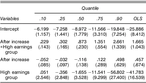
Table 2. Quantile Regression Coef’cients for Duration, Kentucky High and Low Earnings Groups Pooled
Quantile
Variables .10 .25 .50 .75 .90 OLS
Intercept ƒ60199 ƒ70258 ƒ80972ƒ110566ƒ190848ƒ250886
NOTE: The dependent variable is duration (in weeks). The sample size is 5,349. The addi-tional regressors are the same as those in Table 1. The omitted industry is other industries, and the omitted injury is other injuries.
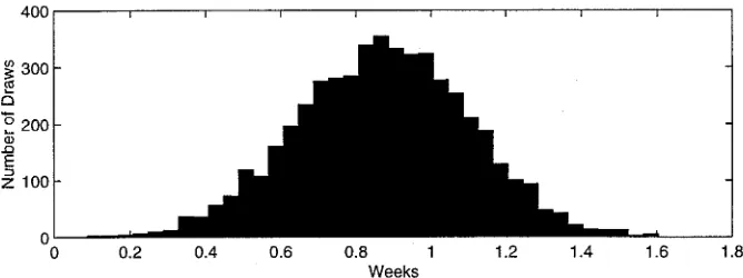
Figure 1. Posterior Histogram.qD.5 (long list forx).
x3D1 if high earnings group,x3D0 otherwise. The key
coef-cient is‚2, measuring the effect of the benet increase on
time out of work, with controls for period and for the earnings group:
‚2D6Eˆ4Y —x2D11 x3D15ƒEˆ4Y —x2D01 x3D157
ƒ6Eˆ4Y—x2D11 x3D05ƒEˆ4Y—x2D01 x3D0570
An appealing aspect of the Meyer et al. analysis is that it is plausible to regard the injury date, and hence the applicable benet schedule, as if it were randomly assigned.
To account for possible changes in the composition of the sample after the benet increase, Meyer et al. included regres-sion controls for attributes of the individual, the job, and the injury—16 regressors in addition to the 4 in (7). The last column of Table 1 presents least squares estimates (and con-ventional standard errors) corresponding to Table 6 in the Meyer et al. work. The rst ve columns of Table 1 present estimates of the linear predictor coefcients corresponding to the 0101 0251 0501 075, and .90 quantiles. These estimates are based on the simulation procedure described earlier. The point estimates are posterior medians, and the standard errors in parentheses are constructed so that the point estimate plus or minus 1.96 standard errors gives an interval with a .95 poste-rior probability. The key coefcients [corresponding to‚2 in
(7)] are in the second row. The effect of the benet increase is fairly constant across the quantiles, suggesting a location model in which the distribution of log duration shifts rigidly in response to the benet increase.
Figure 2. Posterior Histogram.qD.5 (short list forx).
Table 2 presents results using duration out of work (in weeks) instead of its logarithm. Now the estimates show a substantial increase as we go from low to high quantiles, sug-gesting that the effect of the benet increase is concentrated on the upper half of the duration distribution. The estimated effect on the median of the distribution is .87 weeks, with a standard error of .23. In contrast, the least squares estimate of the effect on the mean of the distribution is quite imprecise, with a point estimate of 1.66 and a standard error of 1.04.
The histogram of the draws from the posterior distribution of‚2is shown in Figure 1 for’D05, using duration in weeks. The posterior mean is .87, and the posterior standard deviation is .23. Thus assuming the posterior distribution is normal and using087 1096023 gives a probability interval close to the one we constructed without assuming normality.
We examine the inuence of the prior distribution by cal-culating the expected posterior distribution N‚
m as in (6), for mD21 observations, and comparing this distribution with the posterior distribution‚
n4¢—d5based on the full sample with
nD51349 observations. Here are some of the quantiles of the ‚2distributions for’D05, using duration in weeks:
quantile2 0025 005 025 050 075 095 09751
N ‚2
212 ƒ290 ƒ157 ƒ2004 1001 2403 184 3231
‚2
n 4¢—d52 041 049 071 087 1003 1025 10320
The prior distribution is dominated by the sample information. Now consider dropping all the predictor variables except for the four that appear in 4752 11 x2¢x31 x21 x3. We compare
Chamberlain and Imbens: Nonparametric Applications of Bayesian Inference 17
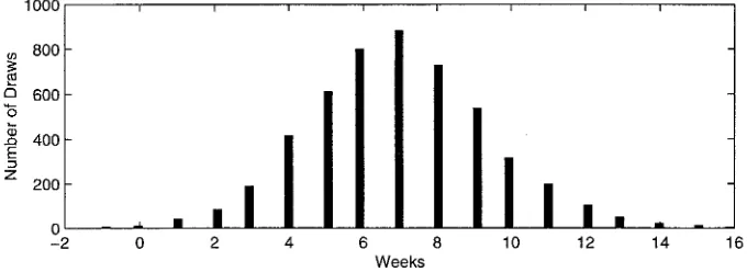
Figure 3. Posterior Histogram.qD.9 (short list forx).
the expected posterior distribution formD5 observations with the posterior distribution based on the full sample. Here are quantiles of these distributions for‚2with’D05, using
dura-tion in weeks:
quantile2 0025 005 025 050 075 095 09751
N ‚2
5 2 ƒ121 ƒ36 ƒ6 1 9 59 1101
‚2
n 4¢—d52 0 0 1 1 2 2 20
The posterior histogram for‚2is in Figure 2. It is concentrated on just four points:ƒ11011, and 2 weeks, with posterior prob-abilities of0011 0141 055, and .30. This reects the discreteness of the benet duration distribution. The upper tail of that dis-tribution is somewhat continuous, but 56% of the distribu-tion is concentrated on the integers from 0 to 4 weeks. The (051 0751 091 0951 0975) quantiles are (418115125149) weeks. Including the long list of predictor variables smoothes out this discreteness in the outcome variable, in the sense of produc-ing a residual distribution (forYƒ‚0X) that is much closer to being continuous.
Here are the quantiles of the ‚2 distributions for ’D09, using just the four regressors in (7) and duration in weeks:
quantile2 0025 005 025 050 075 095 09751
N ‚2
5 2 ƒ145 ƒ41 ƒ7 1 10 72 1241
‚2
n 4¢—d52 2 3 5 7 8 11 120
The posterior histogram for‚2is in Figure 3. This is closer to
a normal distribution, corresponding to the continuity in the upper tail of the duration distribution.
The standard asymptotic distribution theory for quantile regression requires that the distribution of the residualYƒ‚0X (conditional on ˆ) be absolutely continuous with a positive density in a neighborhood of zero. This requirement may be satised because the distribution ofY conditional onX is con-tinuous. Alternatively, even ifY is discrete, it may be satis-ed becauseX0‚ is continuous. For example, with Y binary andX uniform on [011], and E6Y —X7DX, the limiting dis-tribution of the coefcient in a quantile regression is normal despite the binary nature ofY. In our exampleY is discrete with most mass concentrated on a few values. With only three binary regressors, the resulting distribution of the residual is still highly discrete. With the long list of regressors, although many of them are discrete, the continuity requirement for the
residual is much closer to being satised, and the standard large sample approximation to the sampling distribution is more accurate. In contrast, our posterior distributions provide straightforward inferences that do not rely on the approximate normality of a sampling distribution.
4. CONCLUSION
The Bayesian approach to inference provides an attractive conceptual framework because of its connection with opti-mization concepts in decision theory and its lack of reliance on large-sample approximations. In practice, its use has been lim-ited by the requirement of a fully specied parametric model because many econometric models are only partly specied. In this article we presented two applications of a less paramet-ric Bayes approach that are due to Ferguson (1973, 1974) and Rubin (1981). In the rst application, the decision-theoretic nature of the underlying question forces the use of posterior distributions rather than sampling distributions. In the second application, the assumptions underlying the asymptotic nor-mality of the sampling distributions are clearly violated, but inference based on posterior distributions is straightforward.
ACKNOWLEDGMENTS
The authors thank David Cox, Jinyong Hahn, and Neil Shephard for helpful comments and Alan Krueger and Bruce Meyer for making their data available to us. The National Sci-ence Foundation provided nancial support.
[Received December 2000. Revised June 2001.]
REFERENCES
Angrist, J., and Krueger, A. (1991), “Does Compulsory School Attendance Affect Schooling and Earnings?,”Quarterly Journal of Economics, 106, 979–1014.
Barberis, N. (2000), “Investing for the Long Run when Returns are Pre-dictable,”Journal of Finance, 55, 225–264.
Barrodale, I., and Roberts, F. (1973), “An Improved Algorithm for Discretel1 Linear Approximation,”SIAM Journal of Numerical Analysis, 10, 839–848. Chamberlain, G., and Imbens, G. (1995), “Semiparametric Applications of Bayesian Inference,” Discussion Paper 1716, Harvard Institute of Economic Research Cambridge, MA.
Ferguson, T. (1973), “A Bayesian Analysis of Some Nonparametric Prob-lems,”The Annals of Statistics, 1, 209–230.
Ferguson, T. (1974), “Prior Distributions on Spaces of Probability Measures,”
The Annals of Statistics, 2, 615–629.
Hirano, K. (2002), “Semiparametric Bayesian Inference in Autoregressive Panel Data Models,”Econometrica, 70, 781–800.
Kandel, S., and Stambaugh, R. (1996), “On the Predictability of Stock Returns: An Asset-Allocation Perspective,”Journal of Finance, 51, 385–424. Koenker, R., and Bassett, G. (1978), “Regression Quantiles,”Econometrica,
46, 33–50.
Koenker, R., and Bassett, G. (1982), “Robust Tests for Heteroscedasticity Based on Regression Quantiles,”Econometrica, 50, 43–61.
Lancaster, T. (1994), “Bayes WESML: Posterior Inference From Choice-Based Samples,” unpublished manuscript, Brown University, Providence, RI.
Meyer, B., Viscusi, W. K., and Durbin, D. (1995), “Workers’ Compensation and Injury Duration: Evidence From a Natural Experiment,”American Eco-nomic Review, 85, 322–340.
Rossi, P., McCulloch, R., and Allenby, G. (1995), “Hierarchical Modelling of Consumer Heterogeneity: An Application to Target Marketing,” inCase Studies in Bayesian Statistics(Vol. II),Lecture Notes in Statistics, 105, eds. C. Gatsonis, J. Hodges, R. Kass, and N. Singpurwalla, New York: Springer-Verlag, 323–349.
Rubin, D. (1981), “The Bayesian Bootstrap,” The Annals of Statistics, 9, 130–134.