Full Terms & Conditions of access and use can be found at
http://www.tandfonline.com/action/journalInformation?journalCode=ubes20
Download by: [Universitas Maritim Raja Ali Haji] Date: 13 January 2016, At: 01:03
Journal of Business & Economic Statistics
ISSN: 0735-0015 (Print) 1537-2707 (Online) Journal homepage: http://www.tandfonline.com/loi/ubes20
Seasonality Tests
Fabio Busetti & Andrew Harvey
To cite this article: Fabio Busetti & Andrew Harvey (2003) Seasonality Tests, Journal of Business & Economic Statistics, 21:3, 420-436, DOI: 10.1198/073500103288619061
To link to this article: http://dx.doi.org/10.1198/073500103288619061
View supplementary material
Published online: 01 Jan 2012.
Submit your article to this journal
Article views: 80
View related articles
Seasonality Tests
Fabio B
USETTIResearch Department, Bank of Italy, 00184 Rome, Italy (busetti.fabio@insedia.interbusiness.it)
Andrew H
ARVEYFaculty of Economics and Politics, University of Cambridge, Cambridge CB3 9DD, U.K. (ach34@econ.cam.ac.uk)
This article modies and extends the test against nonstationary stochastic seasonality proposed by Canova and Hansen. A simplied form of the test statistic in which the nonparametric correction for serial corre-lation is based on estimates of the spectrum at the seasonal frequencies is considered and shown to have the same asymptotic distribution as the original formulation. Under the null hypothesis, the distribution of the seasonality test statistics is not affected by the inclusion of trends, even when modied to allow for structural breaks, or by the inclusion of regressors with nonseasonal unit roots. A parametric version of the test is proposed, and its performance is compared with that of the nonparametric test using Monte Carlo experiments. A test that allows for breaks in the seasonal pattern is then derived. It is shown that its asymptotic distribution is independent of the break point, and its use is illustrated with a series on U.K. marriages. A general test against any form of permanent seasonality, deterministic or stochastic, is suggested and compared with a Wald test for the signicance of xed seasonal dummies. It is noted that tests constructed in a similar way can be used to detect trading-day effects. An appealing feature of the proposed test statistics is that under the null hypothesis, they all have asymptotic distributions belonging to the Cramér–von Mises family.
KEY WORDS: Cramér–von Mises distribution; Locally best invariant test; Seasonal breaks; Structural time series model; Trading-day effects; Unobserved components.
1. INTRODUCTION
Monthly and quarterly economic time series are often subject to seasonal movements. These seasonal patterns tend to evolve over time, and most seasonal adjustment procedures assume that this is the case. However, if the seasonal pattern does not change, it can be modeled by a set of dummy variables. Indeed, a deterministic seasonal pattern can be removed without even estimating a time series model. All that needs to be assumed is the number of times the series needs to be differenced to make it stationary (see Pierce 1978; Harvey 1989, p. 203). Adjusting series in this way may simplify the exploration of relationships between time series.
Canova and Hansen (1995), hereafter denoted by CH, pro-posed a test of the null hypothesis that the seasonal pattern is deterministic against the alternative that it evolves as a non-stationary stochastic process. The test includes a nonparametric correction for serial correlation and seasonal heteroscedasticity. The aim of this article is to extend the CH test in various direc-tions. We show how to modify the test so as to allow for the effect of modeling breaks in the seasonal pattern. We then con-sider a different, but related testing problem—namely, testing for the presence of any kind of seasonal effects, whether de-terministic, stochastic, or both. Similar techniques can be used for detecting trading-day effects. Before describing these ex-tensions, we examine the CH test in more detail, look at some alternative formulations, and compare the performance of the nonparametric and parametric tests.
Section 2 shows how a nonparametric correction for serial correlation can be set up in terms of the spectrum at seasonal frequencies. This formulation is more restrictive than the CH test insofar as it does not allow for seasonal heteroscedastic-ity. Subject to this proviso, its asymptotic distribution under the null hypothesisis the same as in the original formulation, but its
interpretation is more transparent. In deriving asymptotic distri-butions, we relax the conditions of CH by showing that the dis-tribution is unaffected when a deterministic trend is included in the model; regressors with unit roots can also be included provided that they do not have seasonal unit roots.
Parametric versions of the tests against nonstationary season-ality can be based on structural time series models. Such models are set up in terms of unobserved components, such as trends and cycles, which have a direct interpretation (see Harvey 1989; Kitagawa and Gersch 1996). The use of autoregressive models (as in Caner 1998) is less appealing in this context, because they may yield a poor approximation to the moving average terms typically found in the reduced forms of structural models (see also Taylor 2002a). The evidence provided by Leybourne and McCabe (1994) and Harvey and Streibel (1997) suggests that when testing against the presence of a random walk compo-nent, a parametric approach will usually give tests with a higher power and more reliable size. We investigate whether this is the case for seasonality tests through a series of Monte Carlo ex-periments. The results are reported in the nal section. Along with casting light on the relationship between parametric and nonparametric tests, these experiments provide information on the robustness of the nonparametric test to the order of differ-encing.
Breaks in the trend leave the asymptotic distribution unaf-fected if they are correctly modeled by the inclusion of dummy variables; this is proved in Section 2. Structural breaks in the seasonal pattern are also considered. Empirical results of Canova and Ghysels (1994) suggest that seasonal mean shifts are not uncommon in U.S. quarterly series. Neglecting these
© 2003 American Statistical Association Journal of Business & Economic Statistics July 2003, Vol. 21, No. 3 DOI 10.1198/073500103288619061
420
shifts will bias the nonstationarity tests at both the 0 and the seasonal frequencies. Modeling breaks in the seasonal pattern will, however, affect the distribution of the seasonality test sta-tistics. Section 3 shows how to construct a test statistic against stochastic seasonality, the asymptotic distribution of which is independent of the breakpoint location.
The parametric and nonparametric tests, with the breakpoint modication, are illustrated by an application to a quarterly se-ries on U.K. marriages. The point about this example is that there is an identiable break in the seasonal pattern because of a known change in the tax laws. The modied test is trying to assess whether it is necessary to allow for stochastic season-ality once the deterministic break has been accounted for by intervention dummy variables.
Section 4 suggests a general test for seasonality. This takes the same form as the test against nonstationary seasonality, ex-cept that seasonal dummies are not tted. The asymptotic dis-tribution is given, and the performance of the test is compared with that of a Wald test for the signicance of xed seasonal dummies. Similar techniques are used to construct a test for the presence of trading-day effects.
A unifying feature of the test statistics is that under the null hypothesis, they all have asymptotic distributions belonging to the Cramér–von Mises family. These distributions differ ac-cording to the deterministic components tted and a degrees of freedom parameter. The same distributions arise in tests against nonstationary trends as noted by Harvey (2001).
2. TESTING AGAINST THE PRESENCE OF A
NONSTATIONARY SEASONAL COMPONENT
In this section we develop the trigonometric form of the test against nonstationary stochastic seasonality, show that it is lo-cally best invariant, give nonparametric corrections for serial correlation, and show how to set up a parametric test. We then use Monte Carlo simulation experiments to compare the per-formance of the parametric and nonparametric tests in small samples.
2.1 The Testing Framework
Let yt be a scalar time series, let s denote the number of seasons in a year and let Zt D.z01t; : : : ;z0[s=2]t/0 be an (s¡1) vector of trigonometric seasonal variables, that is,
zjtD.cos 2¼jt=s;sin 2¼jt=s/0,jD1; : : : ;s¤, wheres¤Ds=2¡1 if sis even or [s=2] ifsis odd, whereaszs=2;tD.¡1/t ifs is even. The jth pair of trigonometric terms, zjt, corresponds to thejth harmonic seasonal frequency,¸j´2¼j=s,jD1; : : : ;s¤. Whensis even, the last element ofZt;z[s=2]t, corresponds to the Nyquist frequency,¸[s=2]´¼.
The test against stochastic seasonality is developed in the context of the following unobserved components model:
ytD¹tCstC"t; tD1; : : : ;T; (1)
¹tDXt0¯; (2)
stDZt0°t; (3)
and
A0°tDA0°t¡1C·t; (4)
whereXt is ap£1 vector of linearly independent determinis-tic regressors with associated coefcient vector¯;stis a time-varying seasonal component withZt dened as earlier,Ais a known.s¡1/£kselection matrix with rank k·s¡1, and "t and·t are mutually uncorrelated mean 0 disturbances with variances¾"2 and¾·2W. The initial value°0 is assumed to be
xed.
The aim is to test the null hypothesis that the seasonal com-ponent is deterministic,H0:¾·2D0, against the alternative that it has unit root behavior,H1:¾·2>0. Following CH, the matrix
Ais used to formulate tests at subsets of the seasonal frequen-cies¸1; : : : ; ¸[s=2]. If the test is to be carried out at the single
frequency¸j, then we letAj denote the.2j¡1/th and.2j/th columns ofIs¡1forj<s=2 and the.2j¡1/th column ofIs¡1if jDs=2;Ikdenotes an identity matrix of dimensionk. When all of the seasonal frequencies are considered,ADIs¡1.
2.2 Locally Best Invariant Test
Under Gaussianity, the locally best invariant (LBI) test for the null hypothesis of deterministic seasonality for the model (1)–(4) can be easily obtained from the results of King and Hillier (1985) [which also show that the test is a one-sided La-grange Multiplier (LM) test] and Taylor (2003a).
Specically, letet;tD1; : : : ;T, be the ordinary least squares (OLS) residuals from regressingyt on .Xt0;Zt0/0 and let ¾O2D T¡1PTtD1et2be their sample variance. LetajD1 ifjDs=2 and ajD2 otherwise.
First, consider each seasonal frequency,¸j;jD1; : : : ;[s=2] in turn, that isADAj, in the model (1)–(4). Then, under Gaus-sianity, the LBI test for testingH0:¾·2D0 againstH1:¾·2>0 rejects for large values of the statistic!j, dened as
!jDajT¡2¾O¡2 T
X
tD1
"Á t X
iD1
eicos¸ji
!2
C
Á t X
iD1
eisin¸ji
!2#
;
jD1; : : : ;[s=2]: (5)
Note that whensis even, the test statistic at the Nyquist fre-quency,!s=2, can be written without the termseisin¸s=2i,
be-cause they are identically 0.
A complete test against nonstationary seasonality at all fre-quencies, (i.e.,ADIs¡1) rejects for large values of the statistic
obtained by adding up the test statistics for each individual fre-quency, namely
!D
[Xs=2]
jD1
!j: (6)
This test is LBI for a model where under the alternative hypoth-esis, the coefcients corresponding to each seasonal frequency ¸j;jD1; : : : ;s¤, evolve as mutually independent random walks with variances¾·2, and ifsis even, then the coefcient for fre-quency¼ is a random walk with variance¾·2=2. ThusW is an identity matrix unlesssis even, in which case the last element in the main diagonal is 1/2.
Under H0; !j d
! CvM.aj/ and !
d
! CvM.s¡1/, where
CvM.k/denotes a Cramér–von Mises random variable withk
degrees of freedom andP[jDs=12]ajDs¡1. Gaussianity of the"t’s
is not needed; all that is required is that they be martingale dif-ferences satisfying the conditions of Andrews (1991, p. 823) or Stock (1994, p. 2745). The proof is a special case of Proposition 1 in the next section.
2.3 Nonparametric Correction for Serial Correlation Based on the Spectrum at Seasonal Frequencies
Serial correlation in the stationary component of (1)–(4) can be treated nonparametrically by replacing the sample vari-ance,¾O2, in!j with an estimator of the spectrum of"t at fre-quency¸j. We denote thisspectral nonparametrictest statistic by
!j.m/D
ajPTtD1
£
.PtiD1eicos¸ji/2C.PtiD1eisin¸ji/2
¤
T2gO.¸ jIm/
;
jD1; : : : ;[s=2]; (7)
where
O
g.¸jIm/D m
X
¿D¡m
w.¿;m/°Oe.¿ /cos¸k¿ (8)
is the estimator of the spectral generating function, w.¿;m/ is a weighting function or kernel, such as w.¿;m/D1¡ j¿j= .mC1/, and °Oe.¿ /DT¡1PTtD¿C1etet¡¿ is the sample auto-covariance of the OLS residuals at lag ¿. Alternative options for the kernel w.¢;¢/have been examined by Andrews (1991, p. 821). For testing all of the seasonal frequencies, the spectral nonparametric statistic is
!.m/D
[Xs=2]
jD1
!j.m/:
Under the assumptions set out later, the asymptotic distrib-utions of the foregoing test statistics under the null hypothesis are the same as given in the preceding section.
Assumption A1. Xtis ap£1 vector of deterministic regres-sors, andDT is a (diagonal) scaling matrix such that
.a/ lim T!1T
¡1 T
X
tD1
D¡T1XtX0tD¡T1DQx
and
.b/ lim T!1T
¡1 T
X
tD1
D¡T1XtZ0tD0;
whereQxis a positive denite matrix.
Assumption A2. The "t’s have the structure of a linear process, "t Dà .L/"¤t, where f"¤tg is a martingale difference sequence satisfying the conditions of Stock (1994, p. 2745) and à .L/´1CPi1D1ÃiLi is a polynomial in L, the con-ventional lag operator, Lkyt ´ yt¡k, k D 0;1; : : :, satisfy-ing (a) à .expf§i2¼ ¸j=sg/ 6D0 for all jD1; : : : ;[s=2] and (b)P1kD1kjÃkj<1.
Assumption A3. The lag truncation parameter, m, is such that, asT! 1,m! 1andm=T1=2!0.
Proposition 1. Letytbe generated by the model (1)–(4) un-der the assumptions A1–A3. Then, unun-derH0:¾·2D0, when
ADAj,jD1; : : : ;[s=2],
!j.m/ d
!
Z 1
0
Baj.r/0Baj.r/´CvM.aj/;
whenADIs¡1; !.m/ d
!CvM.s¡1/, whereBk.r/DWk.r/¡ rWk.1/, and Wk.r/, r2[0;1], denotes a k-dimensional stan-dard Wiener process. UnderHA :¾·2>0 and when ADAj, jD1; : : : ;[s=2],!j.m/and!.m/areOp.T=m/.
Proposition 1 extends the results given by CH to allow for a general specication for the deterministic trend¹t; CH gave¹t as a constant level. The limiting distribution is unchanged pro-vided that the regressorsXtsatisfy assumption A1. In particular, contrary to what CH (p. 238) stated, the model can include lin-ear trends. Structural breaks in the trend at known points can also be included. Thus ifXtD.1;t;dt.®//, where dt.®/ is a dummy variable equal to 1 fort> ®Twith 0< ® <1 and equal to 0 fort·®T, then assumption A1 is satised by choosing
DTDdiag.1;T;1/.
Concerning the properties of the disturbances,"t, condition (a) of assumption A2 rules out a 0 in the spectrum at any of the seasonal frequencies¸j,jD1; : : : ;[s=2], whereas condition (b) ensures that poles do not exist in the spectrum. These conditions are satised by any nite-order stationary and invertible ARMA processes. Assumption A3 is required to achieve consistency of the test under the (xed) alternativeHA:¾·2>0 (see Stock 1994, pp. 2797–2799).
Model (1)–(4) can be extended by including stochastic re-gressors with nonseasonal unit roots, and following the line of the proof of Proposition 1, it can be shown that the asymp-totic critical values for the tests in the augmented model are unchanged; the proof is omitted here but is available from the authors on request. Such regressors were ruled out by CH, who stated that “the explanatory variables may be any non-trending variables that satisfy weak dependence conditions.” The gen-eralization is of some practical importance. Note that the pres-ence of cross-correlation between"tand the disturbance vector driving the stochastic regressors is not important for our testing seasonality; unless we are interested in making inferences on the coefcient vector of the regressors, there is no need to use, say, a fully modied least squares procedure instead of OLS.
In summary, the inclusion of deterministic trends and sto-chastic integrated regressors does not affect the asymptotic dis-tribution of the seasonal test statistics. However, the inclusion of seasonal slopes does affect the distribution, just as it does for tests of seasonal unit roots, as discussed by Smith and Tay-lor (1998) and TayTay-lor (2003a). Given the obvious parallels with stationarity tests, it is not difcult to see that the change in dis-tribution is the same as when a time trend is tted before a sta-tionarity test statistic is constructed. The critical values, once again from the Cramér–von Mises family, are as in table 2 of Nyblom and Harvey (2000). For quarterly data, the 5% critical value for an overall test, based on 3 df, is .337. (There is actu-ally a typographical error in the published table, with the value printed as .332.)
Dummy variables introduced to capture breaks in the sea-sonal pattern will also affect the distribution of test statistics. This is the subject of Section 3.
2.4 The Canova–Hansen Test Statistic
The test statistic proposed by CH in the framework of (1)–(4) takes the form
!A.m/DT¡2trace
Á ¡
A0Ä.bm/A¢¡1A0 T
X
tD1 StS0tA
!
; (9)
where StD
Pt
iD1Ziei andbÄ.m/is a nonparametric estimator of the “long run variance” ofZt"t; that is,
b
Ä.m/D
m
X
¿D¡m
w.¿;m/b0.¿ /; (10)
where w.¿;m/ is a kernel as in (8), and b0.¿ / D T¡1
PT
tD¿C1Ztetet¡¿Zt0¡¿ is the sample autocovariance matrix at lag ¿ formed from Ztet. The main difference between (9) and !.m/ is that (9) allows for seasonal heteroscedasticity as in Andrews (1991, p. 839); see CH (p. 240). Under the null hypothesisH0:¾·2D0, the asymptotic representation of (9) corresponds to that of Proposition 2, that is, !A.m/
d
!
CvM.rank.A//.
2.5 Parametric Tests
A structural time series model typically contains stochastic trend and seasonal components, together with an irregular. This model can be extended in various ways; for example, by in-cluding a cycle. However, for many economic time series, the exibility of the stochastic trend is such that the model can still adequately capture seasonal movements if a cycle is excluded. We now consider how to set up a parametric test of whether the seasonal component in a structural time series model is stochas-tic.
If the process generating the nonseasonal part of the model is known, then the LBI test against stochastic seasonality is con-structed from a set of “smoothing errors.” As shown in Appen-dix B, the smoothing errors are in general serially correlated, but the form of this serial correlation may be deduced from the specication of the model, thereby allowing construction of a statistic with a Cramér–von Mises distribution asymptotically, under the null hypothesis. The computation of smoothing er-rors has been discussed by de Jong and Penzer (1998), but if the model contains a serially uncorrelated irregular component, then it can be shown that the smoothing errors are proportional to the optimal estimates of this component.
An alternative possibility is to use theT standardized one-step-ahead prediction errors, the innovations, calculated by treating nonstationary and deterministic components as having xed initial conditions. No correction is then needed; the sta-tistic is of the form (5) and has the same asymptotic distribu-tion. Calculating innovations under the assumption that the ini-tial conditions are xed requires that the iniini-tial conditions be estimated, but a backward smoothing recursion can be avoided simply by reversing the order of the observations and calculat-ing a set of innovations startcalculat-ing from the ltered estimator of the state at the end of the sample. Actually, the forward and backward innovations are not the same, and in neither case do the sums, weighted by cos¸jtand sin¸jt, equal 0, so statistics
formed from forward and backward sums are different. Fortu-nately, the asymptotic properties are unaffected. Smoothing er-rors do not suffer from these ambiguities.
For both the smoothing error and innovation forms of the test, nuisance parameters normally will have to be estimated. For stationarity tests, Leybourne and McCabe (1994) argued that this is best done under the alternative using maximum like-lihood. Proceeding in this way has the compensating advantage that because there often will be some doubt about a suitable model specication, estimation of the unrestricted model af-fords the opportunity to check its suitability by the usual diag-nostics and goodness-of-t tests. Once the nuisance parameters have been estimated, the test statistic is calculated from the in-novations obtained with¾·2set to 0. The asymptotic distribution under the null is unaffected.
2.6 Monte Carlo Experiments
This section compares the probability of rejecting the null hypothesis of constant seasonality for the nonparametric tests of Sections 2.3–2.4 and for the parametric test of Section 2.5 based on a correctly specied model. The results offer guidance in assessing the effectiveness of the two approaches as well as establishing the reliability of the tests in terms of actual, as op-posed to nominal, size.
The data-generation process is the basic structural model (BSM), consisting of seasonal and stationary components com-bined with a local linear trend,¹t. Thus
ytD¹tCZt0°tC"t; "t»NID.0; ¾"2/; tD1; : : : ;T; (11)
where
¹tD¹t¡1C¯t¡1C´t; ´t»NID.0; ¾´2/ (12)
and
¯tD¯t¡1C³t; ³t»NID.0; ¾³2/; (13)
with°tas in (4) withADWDI. The relationship between this seasonal model and the one of Harvey (1989, chap. 2) has been discussed by Proietti (2000).
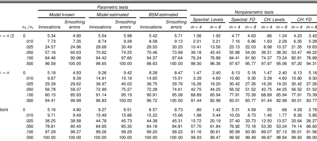
The probability of rejection depends on the seasonal signal-to-noise ratio,q· D¾·2=¾"2, although in the tables we prefer to report the square root. Empirical size and power of the tests are computed for¾·=¾" taking the values 0; :01; :025; :05; :1, and .5. The results are for quarterly series of lengthT D200. The empirical rejection frequencies, reported in percentages, are based on 50,000 replications and refer to tests run at the 5% signicance level. Results for testing at a single frequency, ¼=2 and ¼ in turn, and for the joint test at both frequencies are provided. The program was written in Ox using the SSF-pack set of subroutines of Koopman, Shephard, and Doornik (1999).
The rst set of experiments, the results of which are given in Tables 1, 2, and 3, is for the data-generating process (11)– (13) with¾³2D0, so the trend is a random walk with constant drift,¯. The performance of the tests does not depend on the value assigned to¯, and so it can be equal to 0. The critical fac-tor in the nuisance parameters is the level signal-to-noise ratio,
q´D¾´2=¾"2, andq
1=2
´ is set to .1 in Table 1, .5 in Table 2, and 1.0 in Table 3.
Table 1. Rejection Frequencies for a Random Walk Drift Plus Noise Model With¾´=¾"D:1
Parametric tests
Nonparametric tests Model known Model estimated BSM estimated
Smoothing Smoothing Smoothing Spectral: Levels Spectral: FD CH: Levels CH: FD
¾·=¾" Innovations errors Innovations errors Innovations errors mD4 mD8 mD4 mD8 mD4 mD8 mD4 mD8
¸D¼=2 0 5:10 4:82 5:63 5:85 5:56 5:42 4:29 4:30 4:75 4:47 3:84 3:24 4:16 3:49 :010 8:52 8:10 9:36 9:97 9:23 9:90 7:31 7:23 7:77 7:31 6:32 5:49 6:74 5:61 :025 26:78 27:50 31:52 33:47 31:23 33:19 24:75 23:93 25:33 24:36 22:52 20:24 23:29 20:42 :050 60:37 64:35 74:13 77:96 74:07 77:78 58:80 56:68 58:78 56:56 56:36 52:43 56:44 52:01 :100 86:27 92:61 95:54 98:31 95:40 98:15 86:92 83:86 85:95 83:27 85:49 81:42 84:54 80:45 :500 96:75 100:00 98:70 100:00 98:70 100:00 98:70 96:71 97:72 95:89 98:41 95:50 97:21 94:37
¸D¼ 0 5:13 4:89 8:58 8:83 6:92 6:96 4:53 4:46 6:46 5:35 4:53 4:46 6:46 5:35 :010 10:01 9:53 14:92 15:26 14:67 15:04 8:61 8:35 11:24 9:71 8:61 8:35 11:24 9:71 :025 30:44 30:77 40:51 41:64 40:33 41:44 27:82 26:54 31:49 28:10 27:82 26:54 31:49 28:10 :050 58:05 60:71 74:66 77:40 74:28 77:04 54:48 50:80 57:46 52:47 54:48 50:80 57:46 52:47 :100 80:64 86:91 91:25 96:00 91:09 95:79 76:73 69:92 78:89 71:23 76:73 69:92 78:89 71:23 :500 94:05 100:00 96:43 100:00 96:50 100:00 92:12 83:20 93:08 83:84 92:12 83:20 93:08 83:84
Joint 0 5:01 4:60 9:58 9:79 7:00 6:91 3:98 3:95 5:28 4:55 3:11 2:45 4:29 2:83 :010 10:32 10:24 15:76 16:23 15:59 16:05 8:61 8:14 10:63 9:28 7:13 5:27 8:93 6:02 :025 40:93 41:66 47:25 48:18 46:99 47:90 36:71 34:61 40:00 36:52 32:84 26:80 35:94 28:88 :050 81:31 82:98 87:19 87:78 86:86 87:38 77:68 74:84 79:27 75:70 75:07 68:70 76:94 69:47 :100 97:76 98:77 99:46 99:52 99:29 99:34 96:32 94:47 96:63 94:63 95:56 92:11 95:85 92:25 :500 100:00 100:00 100:00 100:00 100:00 100:00 99:95 99:53 99:93 99:48 99:96 99:13 99:93 99:07
The spectral nonparametric test and the CH test are ap-plied both to levels and to rst differences with the lag trun-cation parameter, m, set to 4 and 8; CH used 3 and 5 for
T D50 and 150. The parametric test statistics are computed rst assuming that q´ is known (with results in the columns headed “Model known”) and then with ¾2
´ and¾"2 estimated by maximum likelihood under the alternative hypothesis (in columns headed “Model estimated”). In addition, the BSM model is also estimated; that is, the constraint that the slope variance is 0 is not imposed (with the relevant columns headed “BSM estimated”). The parametric test results are shown for innovations, computed starting from a smoothed estimate of the initial conditions, and for smoothing errors; compare Sec-tion 2.5.
The main ndings of Tables 1, 2, and 3 are as follows: a. Although the empirical sizes (rows with¾·=¾"equal to 0) of the parametric tests withq´known are very close to the nom-inal 5%, the tests withq´estimated are somewhat oversized at frequency¼. The parametric joint tests for overall seasonality are similarly oversized, with the actual sizes being around .09 in most cases. It is interesting to note that the autoregression-based tests reported by Caner (1998, table 1) display even more oversizing.
b. There appears a slight power advantage for a parametric test constructed from smoothing errors, rather than from inno-vations, when testing at a single frequency (particularly when the smaller empirical size of the parametric test is taken into account); for example, for¸D¼=2 in Table 1, the estimated
Table 2. Rejection Frequencies for a Random Walk Drift Plus Noise Model With¾´=¾"D:5
Parametric tests
Nonparametric tests Model known Model estimated BSM estimated
Smoothing Smoothing Smoothing Spectral: Levels Spectral: FD CH: Levels CH: FD
¾·=¾" Innovations errors Innovations errors Innovations errors mD4 mD8 mD4 mD8 mD4 mD8 mD4 mD8
¸D¼=2 0 5:34 4:90 5:54 5:98 5:42 5:71 1:06 1:92 4:77 4:63 :86 1:24 4:23 3:42 :010 7:73 7:35 8:74 9:28 8:58 9:13 2:01 3:21 7:16 6:86 1:63 2:29 6:35 5:28 :025 24:57 24:96 28:68 30:49 28:50 30:20 10:41 13:56 23:13 22:03 8:98 10:37 21:35 18:63 :050 57:16 60:63 70:62 74:25 70:46 73:99 39:18 43:43 55:88 54:00 36:51 38:30 53:47 49:22 :100 84:46 90:98 94:42 97:66 94:37 97:64 76:24 76:88 84:41 81:60 74:37 73:24 82:81 78:89 :500 96:58 100:00 98:65 100:00 98:63 100:00 98:30 96:36 97:67 95:77 97:97 95:06 97:20 94:31
¸D¼ 0 5:18 4:93 9:26 9:42 8:28 8:47 1:47 2:40 6:13 5:18 1:47 2:40 6:13 5:18 :010 9:67 9:39 14:91 15:18 14:65 15:01 3:39 4:60 10:80 9:30 3:39 4:60 10:80 9:30 :025 29:39 29:62 38:97 40:02 38:75 39:76 16:26 19:20 30:42 27:26 16:26 19:20 30:42 27:26 :050 56:78 59:37 72:99 75:27 72:28 74:61 42:75 44:25 56:52 51:52 42:75 44:25 56:52 51:52 :100 80:15 85:93 91:14 95:19 90:91 95:08 68:89 65:94 77:91 70:39 68:89 65:94 77:91 70:39 :500 94:41 99:99 96:83 100:00 96:72 100:00 91:44 82:98 93:01 83:77 91:44 82:98 93:01 83:77
Joint 0 5:19 4:60 9:27 9:51 8:57 8:73 :80 1:42 5:31 4:59 :55 :68 4:29 2:79 :010 9:71 9:49 15:49 15:88 15:22 15:66 1:98 3:44 10:03 8:73 1:40 1:77 8:26 5:85 :025 38:25 38:58 44:78 45:73 44:38 45:31 15:72 20:19 37:40 33:73 12:50 13:57 33:64 26:27 :050 78:81 80:40 84:65 85:30 84:18 84:81 57:70 61:84 76:92 73:18 53:30 53:24 74:14 66:60 :100 97:29 98:27 99:26 99:29 99:20 99:22 91:16 90:61 95:99 93:90 89:07 87:13 95:01 91:56 :500 100:00 100:00 100:00 100:00 100:00 100:00 99:93 99:47 99:92 99:49 99:87 98:94 99:93 99:00
Table 3. Rejection Frequencies for a Random Walk Drift Plus Noise Model With¾´=¾"D1
Parametric tests
Nonparametric tests Model known Model estimated BSM estimated
Smoothing Smoothing Smoothing Spectral: Levels Spectral: FD CH: Levels CH: FD
¾·=¾" Innovations errors Innovations errors Innovations errors mD4 mD8 mD4 mD8 mD4 mD8 mD4 mD8
¸D¼=2 0 5:33 4:83 5:33 5:69 4:99 5:35 :16 :54 4:90 4:56 :10 :27 4:17 3:44 :010 7:08 6:60 7:46 7:94 7:07 7:61 :30 1:02 6:61 6:50 :24 :61 5:64 4:64 :025 19:11 19:46 22:73 24:38 22:32 24:22 1:98 4:35 18:50 17:66 1:56 2:76 16:80 14:65 :050 49:25 52:78 61:01 65:18 61:67 65:66 15:46 22:57 48:37 46:47 13:51 18:16 46:35 41:83 :100 79:83 86:35 91:44 95:48 91:64 95:43 52:77 60:19 79:78 77:15 50:13 54:99 78:28 73:97 :500 95:77 100:00 98:26 100:00 98:24 100:00 96:92 95:14 97:52 95:48 96:32 93:81 96:94 94:14
¸D¼ 0 5:04 4:82 9:79 9:98 9:45 9:69 :35 :87 5:83 4:91 :35 :87 5:83 4:91 :010 9:20 8:90 14:65 14:97 14:32 14:55 :91 1:77 9:66 8:60 :91 1:77 9:66 8:60 :025 26:84 26:54 35:90 36:82 35:48 36:23 5:92 9:60 27:23 24:57 5:92 9:60 27:23 24:57 :050 53:92 55:70 68:22 70:61 68:29 70:52 24:40 30:80 53:04 48:54 24:40 30:80 53:04 48:54 :100 78:30 83:23 89:99 93:54 90:54 93:51 53:58 56:48 75:69 68:50 53:58 56:48 75:69 68:50 :500 95:01 99:98 96:95 100:00 97:04 99:99 89:56 81:93 92:89 83:65 89:56 81:93 92:89 83:65
Joint 0 4:93 4:49 9:68 9:95 9:27 9:48 :10 :36 4:99 4:54 :03 :12 4:08 2:76 :010 8:61 8:22 14:42 14:91 14:27 14:61 :19 :69 8:96 7:72 :09 :23 7:13 4:76 :025 32:04 31:82 38:92 39:91 38:92 39:65 2:93 6:41 31:43 28:24 2:00 3:45 27:84 21:55 :050 72:27 73:83 78:72 79:39 78:93 79:71 25:60 36:60 70:26 66:48 21:36 27:01 67:22 59:91 :100 95:79 97:10 98:48 98:65 98:16 98:33 72:44 78:29 94:22 91:67 68:82 71:67 92:94 88:96 :500 100:00 100:00 100:00 100:00 100:00 100:00 99:74 99:25 99:92 99:47 99:60 98:58 99:89 98:95
rejection probability is .64 versus .60 when the model is known and .78 versus .74 when the model is estimated. This advantage seems to vanish for the joint tests.
c. Estimating the extra parameter,q³ D¾³2=¾"2 in the more general BSM model has no adverse effect on the performance of the parametric test. On the contrary, there is a slight improve-ment in size in that it is closer to the nominal; for example, in Table 1 the empirical size of the joint test is .07 when a BSM is estimated, compared with .10 when the trend is a random walk with drift.
d. Regarding the nonparametric tests in rst differences, only a small drop in the rejection probabilities occurs when moving from mD4 to mD8. The seasonality test seems less sensitive to lag length than the test of Kwiatkowski, Phillips, Schmidt and Shin (1992); compare the comments of CH (p. 246). However,mshould not be set too small. Our sim-ulations for the joint test withmD0 (unreported in the tables) showed rejection frequencies of 14.5, 13.4, and 11.0 for the models in Tables 1, 2, and 3.
e. The nonparametric test in levels has a much lower proba-bility of rejection than the corresponding test in rst differences whenq1´=2is .5 or 1 (see Tables 2 and 3). This is due to the pres-ence of a so-calledunattended unit rootat frequency 0 when the tests are run in levels. In fact, Busetti and Taylor (2003) and Taylor (2003b) have demonstrated that, although they are con-sistent, the nonparametric tests would suffer from a great loss of power if that unit root were not removed by taking rst dif-ferences of the data. Indeed, these authors showed that under the null hypothesis of deterministic seasonality, the test statis-tics (5), (7), and (9) all converge in probability to 0. This is also conrmed in Tables 1, 2, and 3; in Table 3, where¾´=¾"is equal to 1, the joint test in levels has a size of nearly 0.
f. The parametric tests show higher rejection frequencies than the nonparametric tests, but any assessment of power must be considered in terms of the larger size. Overall, the loss in power resulting from using nonparametric tests is not great. For example, in Table 3,¸D¼=2, where the empirical size of
the innovation-based parametric test is broadly comparable to that of the spectral nonparametric test in rst differences with
mD4, the powers for a seasonal signal-to-noise ratio of .052 are around .60 and .50.
g. The nonparametric tests perform relatively better than the results for stationarity tests (at the 0 frequency) would sug-gest. This is because in the experiments reported in the liter-ature (e.g., Leybourne and McCabe 1994), the process gen-erating the stationary part of the model—typically a rst-order autoregression—interferes with the unit root process. This problem does not arise with the data-generating processes considered here and it would be unlikely to arise even if a rst-order autoregressive process were to replace the white noise ir-regular.
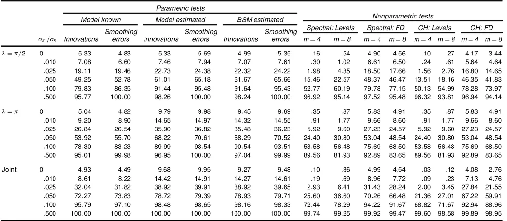
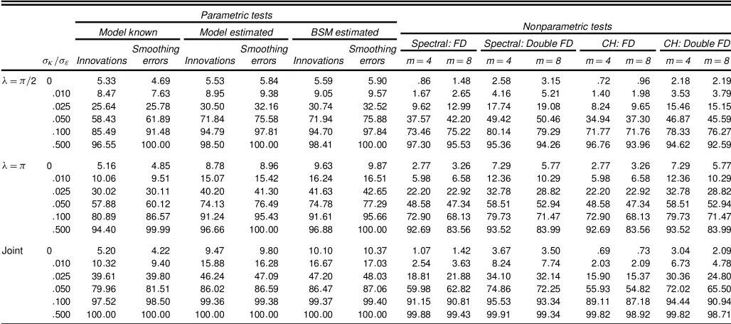
The second group of experiments, reported in Tables 4 and 5, is for the so-called smooth trend model; the data-generating process is given by (11)–(13) with¾´2D0. The relevant signal-to-noise ratio is nowq³. The parametric model is estimated both with and without¾´2set to 0; the results are given in the columns labeled “Model estimated” and “BSM estimated.” The nonpara-metric tests are run after taking rst differences and after taking differences a second time. Although in theory, the rst differ-ence operator should be applied twice to avoid the power loss induced by the presence of unattended unit roots, Table 4 indi-cates that forq1³=2D:1, no signicant loss occurs if only rst differences are taken. In fact, in this case rst differences may be preferable, and becauseq1³=2is often smaller than:1 for eco-nomic time series, basing tests on rst differences may be a good strategy.
The conclusions with respect to size and power that emerge from Tables 4 and 5 are similar to those reached for the ran-dom walk plus drift model of Tables 1, 2, and 3. The parametric tests are somewhat oversized but have a higher probability of rejection under the alternative. Again, there is no disadvantage to tting a more general local linear trend model when carrying out the parametric tests.
Table 4. Rejection Frequencies for a Smooth Trend Plus Noise Model With¾»=¾"D:1
Parametric tests
Nonparametric tests Model known Model estimated BSM estimated
Smoothing Smoothing Smoothing Spectral: FD Spectral: Double FD CH: FD CH: Double FD
¾·=¾" Innovations errors Innovations errors Innovations errors mD4 mD8 mD4 mD8 mD4 mD8 mD4 mD8
¸D¼=2 0 5:36 4:77 5:58 5:86 6:19 6:43 4:22 4:22 2:35 2:96 3:65 3:29 1:92 2:22 :010 8:76 8:11 9:32 9:83 10:06 10:57 7:15 7:05 4:20 5:13 6:17 5:18 3:39 3:71 :025 27:18 27:64 31:82 33:62 33:02 34:94 24:11 23:86 18:19 19:98 22:35 19:59 15:79 15:72 :050 60:56 64:32 74:27 77:68 75:18 78:57 57:76 55:99 50:73 51:80 55:52 51:45 47:95 46:82 :100 86:37 92:50 95:54 98:30 95:59 98:36 85:53 83:07 80:76 79:93 84:15 80:35 79:06 76:93 :500 96:78 100:00 98:68 100:00 98:66 100:00 97:70 95:91 95:43 94:34 97:18 94:36 94:61 92:52 ¸D¼ 0 5:13 4:82 8:66 8:81 9:28 9:44 6:16 5:27 7:41 5:87 6:16 5:27 7:41 5:87 :010 9:99 9:43 14:83 15:12 15:85 16:16 10:85 9:60 12:53 10:52 10:85 9:60 12:53 10:52 :025 30:59 30:82 40:69 41:68 41:78 42:78 30:97 27:80 33:17 29:07 30:97 27:80 33:17 29:07 :050 58:03 60:74 74:38 77:03 74:98 77:95 57:15 52:30 58:90 53:12 57:15 52:30 58:90 53:12 :100 80:72 86:97 91:31 95:73 91:52 95:91 78:63 71:02 79:90 71:60 78:63 71:02 79:90 71:60 :500 94:06 100:00 96:32 100:00 96:38 100:00 93:08 83:82 93:54 84:05 93:08 83:82 93:54 84:05 Joint 0 5:21 4:56 9:49 9:69 10:23 10:53 4:68 4:19 3:67 3:51 3:82 2:64 2:89 2:14 :010 10:65 10:06 15:66 16:02 16:79 17:22 9:82 8:85 8:26 7:81 8:18 5:78 6:91 4:85 :025 41:15 41:44 47:45 48:25 48:95 49:87 38:70 35:77 35:10 32:90 34:31 27:98 31:12 25:48 :050 81:04 82:75 87:35 87:88 87:87 88:42 78:58 75:29 75:91 73:16 75:93 68:87 72:82 66:50 :100 97:82 98:77 99:46 99:53 99:46 99:54 96:48 94:47 95:72 93:86 95:62 92:17 94:70 91:15 :500 100:00 100:00 100:00 100:00 100:00 100:00 99:93 99:48 99:91 99:34 99:92 99:06 99:81 98:73
Because the models used in the foregoing simulations do not exhibit seasonal heteroscedasticity, it is not surprising that the spectral nonparametric test performs slightly better than the CH test. However, once seasonal heteroscedasticity is present, the situation changes. For example, with a model consisting of a seasonal plus white noise with variance in the four quarters of 1, 3, 5, and 7, the size of a!.4/test forTD1;000 was esti-mated to be .080, and that of a!A.4/test was .038. Thus the CH size is closer to the nominal .05. However, withqD:025, the estimated probability of rejection was .458 for!.4/and .662 for!A.4/. Although this is a rather extreme case, it does illus-trate the point that when seasonal heteroscedasticity is present, the CH test not only is more robust with respect to size, but also may show a higher probability of rejection away from the null.
3. DETERMINISTIC BREAKS
IN THE SEASONAL PATTERN
In this section we consider testing against nonstationary sto-chastic seasonality when there is a break in the seasonal pattern at time [®T],®2[0;1]; that is, we replace (3) with
stDZt0°tCdt.®/Zt0µ ; (14)
where dt.®/D1 .t> ®T/ is a break dummy variable. The model now implies that the coefcients of the seasonal terms have changed from°t whent·[®T] to°tCµ whent>[®T]. We focus on the nonparametric tests, although of course the same issues arise with the parametric versions.
Table 5. Rejection Frequencies for a Smooth Trend Plus Noise Model With¾»=¾"D:5
Parametric tests
Nonparametric tests Model known Model estimated BSM estimated
Smoothing Smoothing Smoothing Spectral: FD Spectral: Double FD CH: FD CH: Double FD
¾·=¾" Innovations errors Innovations errors Innovations errors mD4 mD8 mD4 mD8 mD4 mD8 mD4 mD8
¸D¼=2 0 5:33 4:69 5:53 5:84 5:59 5:90 :86 1:48 2:58 3:15 :72 :96 2:18 2:19 :010 8:47 7:63 8:95 9:38 9:05 9:57 1:67 2:65 4:16 5:21 1:40 1:98 3:53 3:79 :025 25:64 25:78 30:50 32:16 30:74 32:52 9:62 12:99 17:74 19:08 8:24 9:65 15:46 15:15 :050 58:43 61:89 71:84 75:58 71:94 75:88 37:57 42:20 49:42 50:46 34:94 37:30 46:87 45:59 :100 85:49 91:48 94:79 97:81 94:70 97:84 73:46 75:22 80:14 79:29 71:77 71:76 78:33 76:27 :500 96:55 100:00 98:50 100:00 98:41 100:00 97:30 95:53 95:36 94:26 96:76 93:96 94:62 92:59
¸D¼ 0 5:16 4:85 8:78 8:96 9:63 9:87 2:77 3:26 7:29 5:77 2:77 3:26 7:29 5:77 :010 10:06 9:51 15:07 15:42 16:24 16:51 5:98 6:58 12:36 10:29 5:98 6:58 12:36 10:29 :025 30:02 30:11 40:20 41:30 41:63 42:65 22:20 22:92 32:78 28:82 22:20 22:92 32:78 28:82 :050 57:88 60:12 74:13 76:49 74:78 77:29 48:58 47:34 58:51 52:94 48:58 47:34 58:51 52:94 :100 80:89 86:57 91:24 95:43 91:61 95:66 72:90 68:13 79:73 71:47 72:90 68:13 79:73 71:47 :500 94:40 99:99 96:66 100:00 96:88 100:00 92:69 83:56 93:52 83:99 92:69 83:56 93:52 83:99
Joint 0 5:20 4:22 9:47 9:80 10:10 10:37 1:07 1:42 3:67 3:50 :69 :73 3:04 2:09 :010 10:32 9:40 15:88 16:28 16:67 17:03 2:54 3:63 8:24 7:74 2:03 2:09 6:73 4:78 :025 39:61 39:80 46:24 47:09 47:20 48:03 18:81 21:88 34:10 32:14 15:90 15:37 30:36 24:80 :050 79:96 81:51 86:02 86:59 86:47 87:06 59:98 62:82 74:86 72:25 55:93 54:82 72:02 65:50 :100 97:52 98:50 99:36 99:38 99:37 99:40 91:15 90:81 95:53 93:34 89:11 87:18 94:44 90:94 :500 100:00 100:00 100:00 100:00 100:00 100:00 99:88 99:43 99:91 99:34 99:82 98:92 99:82 98:71
It is initially assumed that the breakpoint parameter, ®, is known. Extensions to situations in which the breakpoint is un-known are discussed in Section 3.3.
When there is a break in the seasonal pattern, the nonparam-etric test statistics !j.m/, !.m/, and !A.m/ of the preceding section must be constructed using the OLS residuals from re-gressingyt on .Xt0;Zt0;dt.®/Zt0/0. Their asymptotic representa-tions under the null hypothesisare no longer Cramér–von Mises withaj,s¡1,rank.A/df, but rather they depend in a rather complicated way on the breakpoint parameter ®. However, a simple modication yields test statistics, the null limiting dis-tributions of which are still Cramér–von Mises but with degrees of freedom equal to 2aj;2.s¡1/and 2rank.A/. This extends to the seasonal case the modication to the LBI test at frequency 0 suggested by Busetti and Harvey (2001). The parametric test can be modied along the same lines.
3.1 Modied Test With Seasonal Break
The modied seasonal break spectral nonparametric statistic for testing against nonstationary seasonality at frequency¸j is dened as
!¤j.®Im/Daj
PT tD1cjtkt
O
g.¸jIm/
; jD1; : : : ;[s=2]; (15)
where
cjtD
³Xt
iD1
eicos¸ji
´2
C
³Xt
iD1
eisin¸ji
´2
;
ktD[®T]¡2.1¡dt.®//C[.1¡®/T]¡2dt.®/; aj and gO.¸jIm/ are dened as in the preceding section, and the e’ts are the OLS residuals from regressingyt on .Xt0;Zt0; dt.®/Zt0/0. The corresponding statistic for the test at all frequen-cies is then!¤.®Im/DP[jDs=12]!j¤.®Im/. The modications to
the CH statistic, (9), and the parametric statistic are carried out in a similar way.
Proposition 2. Let yt be generated by the model (1), (2), (14), (4) under the assumptions A1–A3. Then, under H0 : ¾·2D0, whenADAj,jD1; : : : ;[s=2],!j¤.®Im/
d
!CvM.2aj/, whenADIs¡1; !¤.®Im/
d
!CvM.2s¡2/. UnderHA:¾·2>0 and whenADAj,jD1; : : : ;[s=2],!j¤.®Im/and!¤.®Im/are Op.T=m/.
The idea behind the construction of (15) is to combine the evidence in the two subsamples, f1; : : : ;[®T]g and f[®T]C 1; : : : ;Tg. Note that !j¤.:5Im/D:25!j.m/; thus when the breakpoint is in the middle of the sample, the tests dened by the two statistics are the same. This is important, because the latter has properties of optimality obtained by extending the LBI/LM test to deal with serial correlation in the stationary component. Furthermore, for the case of testing at frequency 0, Busetti and Harvey (2001) have shown via simulation exper-iments that for®6D:5, the loss of power of the modied test with respect to the LBI test is not great.
3.2 U.K. Marriages
The quarterly series of marriages registered in the United Kingdom from 1958Q1 to 1982Q4 was extracted from various issues of theU.K. Monthly Digest of Statistics. It is shown in Figure 1(a). The spectral nonparametric test statistic,!.m/, cal-culated from rst differences, is 4.18, 2.74, and 2.11 for lags of 4, 8, and 12. This leads to a rejection of the null hypothesis as the 5% critical value for theCvM.3/distribution is 1.00. The original CH statistic, !A.m/, gave smaller values: 1.78, 1.20, and .96.
Estimating (11) with a random walk trend using the STAMP 6 program of Koopman, Harvey, Doornik, and Shephard (2000)
Figure 1. (a) Number of Marriages (in thousands) in the United Kingdom, 1958Q1–1982Q4 and (b) Estimates of the Individual Seasonals.
gives
Q
¾"D0; ¾Q´D1:61; and ¾Q· D2:69; with an equation standard error (the standard deviation of the innovations),¾Q, of 7.91. The parametric test statistic, con-structed from the Kalman lter innovations, is 6.96 which is a much rmer rejection of the null hypothesis than was given by the nonparametric test. The reason for the rejection can be seen in Figure 1(a): there appears to be a break in the seasonal pat-tern at the beginning of 1969. The plot of the individual seasons in Figure 1(b) reveals a switch from winter marriages to mar-riages in the spring quarter. This happened because of a change in the tax law. Up to the end of 1968, couples were allowed to claim the married persons tax allowance retrospectively for the entire year in which they married. Because the tax year begins in April, this arrangement provided an incentive to marry in the rst quarter of the calendar year rather than in the spring.
Adding a set of three seasonal break dummy variables, start-ing in the rst quarter of 1969, to take into account a complete change in the seasonal pattern leads to the following estimates of the parameters:
Q
¾"D2:42; ¾Q´D1:59; and ¾Q· D1:36; with
Q.9;7/D12:54 and ¾Q D5:66;
where Q.P;f/is the Box–Ljung statistic based onPresidual autocorrelations but withf degrees of freedom (see Koopman et al. 2000). Thetstatistics for the seasonal break dummies are
¡8:33, 7.58, and 2.09. There is a large reduction in the estimate of the seasonal parameter,¾·, which no longer needs to allow the stochastic seasonal model to accommodate the change; the equation standard error,¾Q, also is considerably reduced.
The modied seasonal break nonparametric test statistics car-ried out on the residuals obtained from regressing rst differ-ences on seasonal means and the seasonal break dummies are 2.06, 1.69, and 1.58 formD4;8, and 12 for!¤and 1.80, 1.57, and 1.50 for the CH form,!A¤. Thus formD4 and 8, the null of a constant seasonal pattern is rejected by the!¤ test at the 5% level of signicance because the critical value forCvM.6/ is 1.69. However, the smaller values for!¤A lead only to a re-jection formD4. The corresponding parametric test statistic, calculated from the Kalman lter innovations, is 2.42, giving a stronger indication that there is still stochastic seasonality present. This is supported by the fact that estimating the model with a xed seasonal gives a signicant Box–Ljung statistic of
Q.9;8/D22:38, whereas the fourth-order residual autocorrela-tion,r.4/, is .33.
3.3 Unknown Breakpoint
If the breakpoint parameter ® is unknown, then the two-step strategy of Busetti and Harvey (2003) for testing station-arity in the presence of a structural break can be adapted in a straightforward manner. The idea is to estimate the break-point under the null by minimizing, over ®, the error vari-ance of an OLS regression of yt on.Xt0;Zt0;dt.®/Z0t/0, that is,
O
®Darg min®T¡1
PT
tD1e2t, whereetare the OLS residuals. Bai (1997) showed that under the null hypothesis of deterministic
seasonality this estimator is superconsistent in the sense that it converges to the true value at rateT instead of the usual rate
T1=2. Therefore, the null asymptotic distributions of!¤j.®OIm/ and!¤.®OIm/are the same as if the true value® were used, whereas under the alternative hypothesis, the statistics diverge regardless of the break date used due to the presence of the sea-sonal unit roots. Hence running the seasea-sonal break tests with an estimated breakpoint leads to an asymptotically valid proce-dure. Clearly, some loss of power with respect to a test based on a known® is to be expected. Busetti and Harvey (2003) used Monte Carlo simulation experiments to evaluate this power loss for the zero frequency stationarity tests.
4. TESTING AGAINST A PERMANENT
SEASONAL COMPONENT
The test against nonstationary seasonal components takes the null hypothesis to be a model in which seasonality is determin-istic. Sometimes we may wish to test whether there is any sea-sonality at all, irrespective of whether it is deterministic or sto-chastic. One strategy, implemented in the STAMP package, is to t a structural time series model and then perform a test of signicance on the seasonal coefcients as estimated at the end of the period. However, this has the disadvantage of not being able to indicate seasonal effects in a situation where seasonal-ity has become less pronounced over time. This is precisely the kind of behavior noted by CH (pp. 24–50) in their analysis of U.S. macroeconomic series.
4.1 Tests and Their Power
Our aim is to develop tests that are powerful against the pres-ence of deterministic seasonality and/or stochastic seasonality. The stochastic seasonality is taken to be nonstationary, so that the effects arepermanentin that forecasts of the seasonal pat-tern remain constant rather than dying away. We thus consider the data-generating process (1)–(4) withADIs¡1and split the
seasonal component,st, into deterministic and stochastic parts,
stDsDt CsSt; (16)
sDt DZt0°0; (17)
and
sSt DZt0 t
P
iD1
·i; (18)
where °0 is a .s¡1/£1 vector of xed coefcients and·t is a vector of mean 0, serially independent disturbances with covariance matrix¾·2W, independent of"t. The null hypothesis of no seasonality is
H0:°0D0; ¾·2D0;
whereas the alternative hypotheses are of deterministic season-ality,
H1D:°06D0; ¾·2D0;
and stochastic seasonality,
HS1:°0D0; ¾·2>0:
We show in Proposition 3 that the standard Wald test on xed seasonal coefcients is consistent against both alternative hy-potheses. We also show that a test constructed in a similar way to the tests of Section 2, but without tting seasonal regressors, is consistent against both hypotheses. More specically let et be the OLS residuals from regressingyt on.X0t;Zt0/0and letet be the residual from regressingytonXtonly. Because assump-tion A1 requires that the two sets of regressorsXtandZtbe or-thogonal in large samples, theXt0s can be ignored in the analysis of the Wald statistic, which may be written as
FD O°00 the estimator of¾"2. Note that the usual form of theFstatistic is ourFmultiplied by.T¡sC1/=2T. but using the residualset and with the summation running in the reverse order, that is,
!jDajT¡2¾¡2 Hillier (1985) and Taylor (2003a), it is easy to show that when
W is specied as after formula (6), !is the LBI test statistic againstHS
1 for the model in (1)–(4) with°0D0. Note that in
the LBI statistics the summations run in reverse order, from
t to T as opposed from 1 to t; in the tests of Section 1 the reverse summations can be replaced by the more usual direct summations, because tting the seasonal regressors implies that
PT
iD1ZieiD0.
The following proposition provides the asymptotic distri-bution of F and ! under the local alternative hypotheses
H1D;T andH1S;T, whereH1D;T:°0DcD¶= andcSare xed constants. This provides the basis of a power comparison between the two tests.
Proposition 3. Let yt be generated by the model (1)–(2), (16)–(18) with W DIs¡1 and with the nonseasonal
regres-sorsXt satisfying assumption A1 of Section 1. LetW0;s¡1.r/, W1;s¡1.r/be independent standard Wiener processes of
dimen-sions¡1, and let3Ddiag.1=2; : : : ;1=2;1/whensis even and
Remark 1. The asymptotic distribution ofFunderH1D;Tis a noncentral chi-squared distribution withs¡1 df and noncen-trality parameter equal toc2D¶03¶=¾"2.
Remark 2. Under both local alternatives (i.e., when °0D cD¶=
Remark 3. A modication of!would be to replace¾2with
O
¾2, that is, to t seasonal dummies when calculating the
denom-inator of the statistics in (21). This makes no difference to the asymptotic distribution under the null and the local alternative hypotheses.
Although the asymptotic distribution of!under the null hy-pothesis differs from that of!, it still belongs to the Cramér– von Mises family. The 5% critical values for 1, 2, and 3 df— the latter appropriate for a full test on quarterly data—are 1.65, 2.63, and 3.46 (see table 1 of Nyblom 1989, p. 227). The 5% critical value for 11 df (kindly supplied by J. Nyblom) is 9.03. For the reasons given in subsection 2.3, the asymptotic distrib-ution is unaffected by the inclusion of a constant or a constant and a time trend.
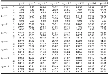
The asymptotic distributions ofF and!under the local al-ternativesH1D;TandH1S;Tcan be used to compare the power per-formance of the two tests. This is done in Table 6. Specically, for a quarterly model,sD4, we have generated 50,000 replica-tions of the limiting random variables dened in Proposition 3 by replacing the continuous-timeWiener processesW0;s¡1, and W1;s¡1by their discrete counterparts (dividing the unit interval
into 1,000 parts). We have also considered the limiting behavior of the!test, invariant to the presence of deterministic seasonal-ity; its asymptotic distribution againstHS1;Twas given by Taylor (2003a). Note that under both the xed and local alternativeHD1
andHD1;T, the asymptotic power of this test is equal to its nomi-nal size.
Thus Table 6 reports, for a quarterly model, the local asymp-totic power of the three tests at the nominal 5% signicance level across a range of values for the parameterscDandcS(with
¾"2set equal to 1). As expected, the Wald test is more powerful under the local alternative of deterministic seasonality, whereas !achieves the highest power under pure stochastic seasonality, being the LBI test for this case. For example, forcDD2 and cSD0, the asymptotic power of the Wald test is .652, as op-posed to .559 for the test based on!. In contrast, forcSD4 and cDD0, the power of the!test is .668, whereas that of the Wald test is .627. Finally, note that under pure stochastic seasonality, the power of the!test of Section 2 is considerably lower than that of!.
Table 6. Local Asymptotic Power Against Deterministic and/or Pure Stochastic Seasonality of the F,!,
and!Tests
cDD0 cDD:5 cDD1:0 cDD1:5 cDD2:0 cDD2:5 cDD3:0 cDD3:5
cSD0 F 4:90 7:98 18:86 39:72 65:21 85:52 95:94 99:26
! 4:90 7:46 16:01 32:90 55:85 77:37 91:33 97:74
! 4:89 4:89 4:89 4:89 4:89 4:89 4:89 4:89
cSD1 F 9:34 12:94 24:52 44:17 66:36 84:43 94:68 98:75
! 10:53 13:60 23:03 39:08 58:60 77:02 89:81 96:60
! 6:08 6:08 6:08 6:08 6:08 6:08 6:08 6:08
cSD2 F 24:52 28:19 38:61 53:51 69:58 83:02 92:33 97:10
! 29:07 31:83 39:84 51:65 65:16 77:85 87:75 94:21
! 10:32 10:32 10:32 10:32 10:32 10:32 10:32 10:32
cSD3 F 45:34 47:74 54:35 63:94 74:19 83:43 90:61 95:34
! 51:46 53:38 58:28 64:92 72:91 80:79 87:45 92:66
! 18:13 18:13 18:13 18:13 18:13 18:13 18:13 18:13
cSD4 F 62:72 63:97 67:81 73:12 79:32 85:26 90:33 94:16
! 68:83 69:70 72:13 75:80 80:10 84:69 88:87 92:51
! 29:22 29:22 29:22 29:22 29:22 29:22 29:22 29:22
cSD5 F 74:79 75:58 77:52 80:63 84:07 87:66 91:06 93:96
! 80:10 80:58 81:76 83:56 85:84 88:55 90:97 93:16
! 41:62 41:62 41:62 41:62 41:62 41:62 41:62 41:62
cSD7:5 F 89:59 89:82 90:27 90:93 91:87 93:01 94:15 95:31
! 92:79 92:84 93:00 93:46 94:02 94:68 95:29 95:97
! 68:11 68:11 68:11 68:11 68:11 68:11 68:11 68:11
cSD10 F 95:09 95:21 95:25 95:49 95:70 96:05 96:45 96:90
! 97:03 97:05 97:08 97:17 97:27 97:44 97:64 97:87
! 83:73 83:73 83:73 83:73 83:73 83:73 83:73 83:73
The local power of the modied test, using¾O2rather than¾2, is, as suggested in Remark 3, the same as that of!. However, in practice it may well have a higher power than!against de-terministic seasonality. This is because when¾·2D0, the prob-ability limit of¾2exceeds that of¾O2; indeed, because¾2¸ O¾2, the modied statistic will always be greater than or equal to!. There is a parallel with the test on°O0in that using¾2instead of
O
¾2would give the LM statistic.
A second modication is also in order. As formulated in (21), the test is LBI against stochastic seasonality with °0D0. In
practice, we are more concerned with seasonal patterns that di-minish over time. Thus our recommendation is to use the for-wardsummation just as in the!test of Section 2, because this would be the LBI test if the data were generated backward start-ing with°TC1D0. Taking these points into consideration, our
preferred statistic,!, is constructed using
!
jDajT ¡2
O
¾¡2
T
X
tD1
"Á t X
iD1
eicos¸ji
!2
C
Á t X
iD1
eisin¸ji
!2#
;
jD1; : : : ;[s=2]: (22)
When"t is serially correlated, the!test can be modied as in Section 2.3. If the spectrum is computed using the residuals after tting the seasonal regressors, then the statistic is denoted by !¤.m/. The test can be extended to deal with both serial correlation and heteroscedasticity by making the amendment of (9).
The Wald test can be carried out by tting a model that is unrestricted except insofar as the seasonal component is taken to be nonstochastic; that is,¾·2is set to 0. Alternatively, a non-parametric test can be set up using a nonnon-parametric covariance
matrix estimator, as was done by Andrews (1991). This is es-sentially the same correction as in (9). To be specic,
F.m/DT°O00[Q¡1bÄ.m/Q¡1]¡1°O0; (23)
whereQDT¡1PtTD1ZtZt0. If there is no need to guard against heteroscedasticity, the modications are made simply using es-timates of the spectrum as for!¤.m/.
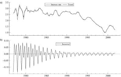
4.2 A Diminishing Seasonal Pattern in Spanish Interest Rates
As an example, we consider the logarithm of 3-month money market interest rate in Spain for the period 1977Q1–2001Q4; the source is the Bank of International Settlements macroeco-nomic series database. The series is depicted in Figure 2(a). It is difcult to detect a seasonal pattern from a casual glance at the graph, and one would not normally expect such a pattern to be present in an interest rate series; however, the functioning of the interbank loans market may imply some seasonality (see, e.g., Hamilton 1996).
Fitting the BSM to the series gives a seasonal component, as shown in Figure 2(b); the slope variance is estimated to be 0, and the estimate of the (xed) slope is small and insignicant. We have used logarithms of the data only because the diag-nostics are better; if the raw series is used, then the resulting seasonal pattern is similar.
The chi-squared statistic for the seasonals at the end of the series is only .09, which is clearly not signicant, because the 5% critical value for aÂ32is 7.81. However, the graph shows a fairly strong seasonal pattern until the mid-1980s. The question is whether the pattern as a whole is in any sense signicant.
Setting the seasonal variance to 0 and reestimating the BSM gives a Wald statistic of 4.76, with apvalue of .19. This is still
Figure 2. (a) Logarithm of the 3-Month Spanish Interest Rate, 1977Q1–2001Q4 and (b) Estimate of the Seasonal Component.
not signicant. If the series is differenced and a nonparametric Wald test, (23), is computed using the Newey–West covariance matrix estimator with three lags, then a similarpvalue (.17) is obtained.On the other hand, the spectral nonparametric statistic computed using forward summations takes the values 3.83 and 3.01 for mD3 and 6, rising to 4.64 and 3.89 for!¤.m/, the preferred form in which the spectrum is estimated after tting seasonal regressors. Because the 5% critical value is 3.46, this test provides a rm rejection of the hypothesis that there is no seasonality in the series.
Finally, formD3 and 6, the!.m/statistic of Section 2 takes the values 1.17 and 1.02 (against a 5% critical value of 1.00). This conrms the presence of stochastic seasonality.
4.3 Seasonal Adjustment
The foregoing tests can be applied to a seasonally adjusted series to check whether the adjustment has been effective. This assumes that the adjustment has been done by means of mov-ing averages, rather than by regressmov-ing on seasonal dummies. If dummies have been used, then the!test statistics have the asymptotic distributions of Section 2.
4.4 Detection of Trading-Day Effects
Cleveland and Devlin (1980) showed that peaks at certain frequencies in the estimated spectra of monthly time series in-dicate the presence of trading-day effects. Specically, there is a peak at a frequency of:348£2¼radians, with the possibility of subsidiary peaks at :432£2¼ and:304£2¼ radians. An option in the output of the X-12-ARIMA program provides a comparison of the estimates of these frequencies with the ad-jacent frequencies (see Soukup and Findley 2000). However, there is no formal test. One possibility is to construct paramet-ric or nonparametparamet-ric statistics analogous to!j and!
j so as to
carry out tests for permanent cyclical effects at one or all of the three trading-day frequencies. Assuming that no (deterministic) trading-day model has been tted, the asymptotic distributions under the null will beCvM0, with a 5% critical value of 2.63 for a test at a single frequency and 5.68 for a test at all three frequencies.
As an example, we took the irregular component, obtained from X12-ARIMA, of series s0b56ym, U.S. Retail Sales of Children’s, Family, and Miscellaneous Apparel, as supplied by the Bureau of the Census. Because the process followed by this irregular component cannot be derived, we decided to use the nonparametric test. The test statistic with 10 lags was 7.03 for the single main frequency and 8.21 for all three frequencies. Both give a clear rejection of the null hypothesis that there is no trading-day effect.
5. CONCLUSION
The seasonality test statistic proposed by CH may be sim-plied so that a nonparametric correction for serial correlation is based on estimating the spectrum of the series at the rele-vant seasonal frequency or frequencies. This test statistic then has a very straightforward interpretation. As might be expected, Monte Carlo experiments show a slight gain in power over the original CH test for homoscedastic series, but a size distortion and lower power when there is seasonal heteroscedasticity.
If a model is tted, then a parametric seasonality test may be based on the innovations or smoothing errors, but Monte Carlo experiments show that they have similar properties. If the main reason for tting a model is to investigate seasonality, then a basic structural time series model consisting of stochastic trend, seasonal, and irregular components usually will be ade-quate. However, it is worth noting that the innovations test can be implemented for any structural time series model, including