Fast Dynamic Speech Recognition via Discrete Tchebichef Transform
Ferda Ernawan, Edi Noersasongko
Faculty of Information and Communication TechnologyUniversitas Dian Nuswantoro (UDINUS) Semarang, Indonesia
e-mail: [email protected], [email protected]
Nur Azman Abu
Faculty of Information and Communication Technology Universiti Teknikal Malaysia Melaka (UTeM)
Melaka, Malaysia e-mail: [email protected]
AbstractTraditionally, speech recognition requires large computational windows. This paper proposes an approach based on 256 discrete orthonormal Tchebichef polynomials for efficient speech recognition. The method uses a simplified set of recurrence relation matrix to compute within each window. Unlike the Fast Fourier Transform (FFT), discrete orthonormal Tchebichef transform (DTT) provides simpler matrix setting which involves real coefficient number only. The comparison among 256 DTT, 1024 DTT and 1024 FFT has been done to recognize five vowels and five consonants. The experimental results show the practical advantage of 256 Discrete Tchebichef Transform in term of spectral frequency and time taken of speech recognition performance. 256 DTT produces frequency formants relatively identical similar output with 1024 DTT and 1024 FFT in term of speech recognition. The 256 DTT has a potential to be a competitive candidate for computationally efficient dynamic speech recognition.
Keywords-speech recognition; fast Fourier transforms; discrete Tchebichef transform.
I. INTRODUCTION
A commonly used FFT requires large sample data for each window. 1024 sample data FFT computation is considered the main basic algorithm for several digital signals processing [1]. In addition, FFT algorithm is computationally complex and it requires especial algorithm on imaginary numbers. Discrete orthonormal Tchebichef transform is proposed here instead of the popular FFT.
The Discrete Tchebichef Transform is a transformation method based on discrete Tchebichef polynomials [2][3]. DTT has lower computational complexity and it does not require complex transform. The original design of DTT does not involve any numerical approximation. The Tchebichef polynomials have unit weight and algebraic recurrence relations involving real coefficient numbers unlike continuous orthonormal transform. The discrete Tchebichef polynomials involve only algebraic expressions; therefore it can be compute easily using a set of recurrence relations. In the previous research, DTT has provided some advantages in spectrum analysis of speech recognition which has the potential to compute more efficiently than FFT [4]-[6]. DTT has been recently applied in several image processing applications. For examples, DTT has been used in image
analysis [7][8], image reconstruction [2][9][10], image projection [11] and image compression [12][13].
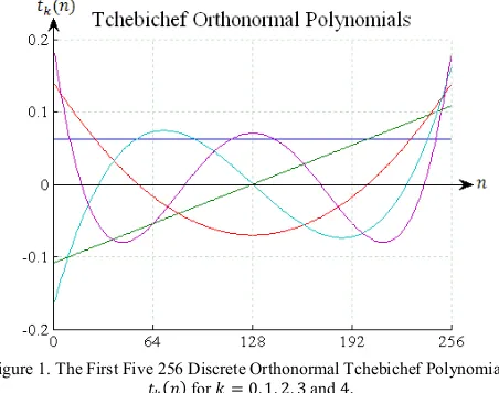
This paper proposes an approach based on 256 discrete orthonormal Tchebichef polynomials as presented in Fig. 1. The smaller matrix of DTT is chosen to get smaller computation in speech recognition process. This paper will analyze power spectral density, frequency formants and speech recognition performance for five vowels and five consonants using 256 discrete orthonormal Tchebichef polynomials.
Figure 1. The First Five 256 Discrete Orthonormal Tchebichef Polynomials ݐሺ݊ሻ for ݇ ൌ Ͳǡ ͳǡ ʹǡ ͵ and ͶǤ
The organization of this paper is as follows. The next section reviews the discrete orthonormal Tchebichef polynomials. The implementation of dicrete orthonormal Tchebichef polynomials shall be given in section III. The section IV discusses comparative analysis of frequency formants and speech recognition performance using 256 DTT, 1024 DTT and 1024 FFT. Finally, section V gives the conclusions.
II. DISCRETE ORTHONORMAL TCHEBICHEF
POLYNOMIALS
Speech recognition requires large sample data in the computation of speech signal processing. To avoid such problem, the orthonormal Tchebichef polynomials use the set recurrence relation to approximate the speech signals. For a given positive integer ܰ (the vector size), and a value ݊ in the rangeሾͳǡ ܰ െ ͳሿ, the orthonormal version of the one 2011 First International Conference on Informatics and Computational Intelligence
dimensional Tchebichef function is given by following recurrence relations in polynomials ݐሺ݊ሻǡ ݊ ൌ ͳǡʹǡ ǥ ǡ ܰ െ ͳ [9]:
ݐሺ݊ሻ ൌξேଵǡ (1)
ݐሺͲሻ ൌඨܰ െ ݇ܰ ݇ඨʹ݇ ͳʹ݇ െ ͳ ݐିଵሺͲሻǡ (2)
ݐሺͳሻ ൌቊͳ ݇ሺͳ ݇ሻͳ െ ܰ ቋ ݐሺͲሻǡ (3)
ݐሺ݊ሻ ൌ ߛଵݐሺ݊ െ ͳሻ ߛଶݐሺ݊ െ ʹሻǡ (4)
݇ ൌ ͳǡ ʹǡ ǥ ǡ ܰ െ ͳǡ ݊ ൌ ʹǡ ͵ǡ ǥ ǡ ቀே
ଶെ ͳቁǡ
where
ߛଵൌെ݇ሺ݇ ͳሻ െ ሺʹ݊ െ ͳሻሺ݊ െ ܰ െ ͳሻ െ ݊݊ሺܰ െ ݊ሻ ǡ (5)
ߛଶൌሺ݊ ͳሻሺ݊ െ ܰ െ ͳሻ݊ሺܰ െ ݊ሻ ǡ (6)
The forward discrete orthonormal Tchebichef polynomials set ݐሺ݊ሻ of order ܰ is defined as:
ܺሺ݇ሻ ൌ ݔሺ݊ሻݐሺ݊ሻǡ ேିଵ
ୀ (7)
݇ ൌ Ͳǡ ͳǡ ǥ ǡ ܰ െ ͳǡ
where ܺሺ݇ሻ denotes the coefficient of orthonormal Tchebichef polynomials. ݊ ൌ Ͳǡ ͳǡ ǥ ǡ ܰ െ ͳǤ ݔሺ݊ሻ is the sample of speech signal at time index ݊Ǥ
III. THE PROPOSED DISCRETE ORTHONORMAL
TCHEBICHEF TRANSFORM FOR SPEECH RECOGNITION
A. Sample Sounds
The sample sounds of five vowels and five consonants used here are male voice from the Acoustic Characteristics of American English Vowels [14] and International Phonetic Alphabet [15] respectively. The sample sounds of vowels and consonants have a sampling rate frequency component at about 10 KHz and 11 KHz. As speech data, there are three of classifying events in speech, which are silence, unvoiced and voiced. By removing the silence part, the speech sound can provide useful information of each utterance. One important threshold is required to remove the silence part. In this experiment, the threshold isͲǤͳ. This means that any zero-crossings that start and end within the range of ݐǡ whereെͲǤͳ ൏ ݐ൏ ͲǤͳ, are to be discarded.
B. Speech Signal Windowed
The samples of five vowels and five consonants have 4096 sample data which representing speech signal. On one hand, the sample of speech signal of vowels and consonants are windowed into four frames. Each frame consumes 1024 sample data which represent speech signal. In this study, the sample speech signal for 1-1024, 1025-2048, 2049-3072, 3073-4096 sample data is represented on frames 1, 2, 3, and
4 respectively. In this experiment, the sample speech signal on fourth frame is used to evaluate and analyze using 1024 DTT and 1024 FFT. On the other hand, the sample speech signals of the vowels and consonants are windowed into sixteen frames. Each window consists of 256 sample data which represents speech signals. In this study, the speech signal of five vowels and five consonants on sixth and fifteen frames respectively is used to analyze using 256 DTT. The sample of speech signal is presented in Fig. 2.
Figure 2. Speech Signal Windowed into Sixteen Frames.
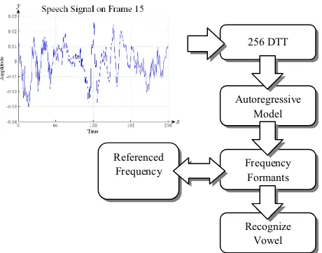
Since we are doing speech recognition in English, the schemes are on the initial and final consonants. Typically an English word has middle silent consonant. it is also critical to provide the dynamic recognition module in making initial guess before final confirmation on the immediate vowel or consonant. The visual representation of speech recognition using DTT is given in Fig. 3.
Figure 3. The Visualization of Speech Recognition Using DTT
The sample frame is computed with 256 discrete Tchebichef Transform. Next, autoregressive is used to generate formants or detect the peaks of the frequency signal. These formants are used to determine the characteristics of the
256 DTT
Autoregressive Model
Frequency Formants
Recognize Vowel Referenced
vocal by comparing to referenced formants. The referenced formants comparison is defined base on the classic study of vowel [16]. Then, the comparison of these formants is to decide the output of vowel or consonant.
C. The Coefficients of Discrete Tchebichef Transform
This section provides a representation of DTT coefficient formula. Consider the discrete orthonormal Tchebichef polynomials definition (1)-(8) above, a set kernel matrix 256 orthonormal polynomials are computed with speech signal on each window. The coefficients of DTT of order n = 256 sample data for each window are given as follow formula:
TC = S (8)
ۏ ێ ێ ێ
ۍ ݐሺͲሻ ݐሺͳሻ
ݐଵሺͲሻ ݐଵሺͳሻ
ݐሺʹሻ ڮ ݐሺ݊ െ ͳሻ
ݐଵሺʹሻ ڮ ݐଵሺ݊ െ ͳሻ
ݐଶሺͲሻ ݐଶሺͳሻ
ڭ ݐିଵሺͲሻ
ڭ ݐିଵሺͳሻ
ݐଶሺʹሻ ڮ ݐଶሺ݊ െ ͳሻ
ڭ ݐିଵሺʹሻ
ڰ
ڮ ݐିଵሺ݊ െ ͳሻےڭ
ۑ ۑ ۑ ې
ۏ ێ ێ ێ ۍ ܿܿଵ
ܿଶ
ڭ ܿିଵےۑ
ۑ ۑ ې
ൌ ۏ ێ ێ ێ ۍ ݔݔଵ
ݔଶ
ڭ ݔିଵےۑ
ۑ ۑ ې
where C is the coefficient of discrete orthonormal Tchebichef polynomials, which representsܿǡ ܿଵǡ ܿଶǡ ǥ ǡ ܿିଵ. T is matrix computation of discrete orthonormal Tchebichef polynomials ݐሺ݊ሻfor݇ ൌ Ͳǡ ͳǡ ʹǡ ǥ ǡ ܰ െ ͳǤS is the sample of speech signal window which is given by ݔሺͲሻǡ ݔሺͳሻǡ ݔሺʹሻǡ ǥ ǡ ݔሺ݊ െ ͳሻ. The coefficient of DTT is given in as follows:
ܥ ൌ ܶିଵܵ (9)
D. Power Spectral Density
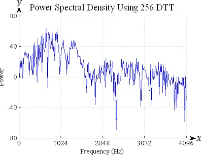
Power Spectral Density (PSD) is the estimation of distribution of power contained in a signal over frequency range [17]. The unit of PSD is energy per frequency. PSD represent the power of amplitude modulation signals. The power spectral density using DTT is given in as follows:
ݓሺ݇ሻ ൌ ʹሺݐȁܿሺ݊ሻȁଶ
ଶെ ݐଵሻ (10)
where ܿሺ݊ሻ is coefficient of dicrete Tchebichef Transform. ሺݐଵǡ ݐଶሻ are precisely the average power of spectrum in the
time range.. The power spectral density using 256 DTT for vowel 'O' and consonant 'RA' are shown in Fig. 4 and Fig. 5.
Figure 4. Power Spectral Density of vowel ‘O’ using 256 DTT
Figure 5. Power Spectral Density of consonant ‘RA’ using 256 DTT
The one-sided PSD using FFT can be computed as:
ݏሺ݇ሻ ൌ ʹሺݐȁܺሺ݇ሻȁଶ
ଶെ ݐଵሻ (11)
where ܺሺ݇ሻ is a vector of ܰ values at frequency index ݇, the factor 2 is due to add for the contributions from positive and negative frequencies. The power spectral density is plotted using a decibel (dB) scaleʹͲ ͳͲ. The power spectral density using FFT for vowel 'O' and consonant ‘RA’ on frame 4 is shown in Fig. 6 and Fig. 7.
Figure 6. Power Spectral Density of vowel ‘O’ using FFT.
E. Autoregressive
Speech production is modeled by excitation filter model, where an autoregressive filter model is used to determine the vocal tract resonance property and an impulse models the excitation of voiced speech [18]. The autoregressive process of a series ݕ using DTT of order v can be expressed in the following equation:
ݕൌ െ ܽ ௩
ୀଵ
ܿି ݁ (12)
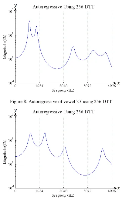
Where ܽ are real value autoregression coefficients, ܿ is the coefficient of DTT at frequency index݆, ݒis 12 and ݁ represent the errors term independent of past samples. The autoregressive using 256 DTT for vowel ‘O’ and consonant ‘RA’ are shown in Fig. 8 and Fig. 9.
Figure 8. Autoregressive of vowel 'O' using 256 DTT
Figure 9. Autoregressive of consonant 'RA' using 256 DTT
Next, the autoregressive process of a series ݕ using FFT of order v is given in the following equation:
ݕൌ െ ܽ ௩
ୀଵ
ݍି ݁ (13)
where ܽ are real value autoregression coefficients, ݍ represent the inverse FFT from power spectral density, and ݒis 12. The peaks of frequency formants using FFT in autoregressive for vowel 'O' and consonant ‘RA’ on frame 4 were shown in Fig. 10 and Fig. 11.
Figure 10. Autoregressive using FFT for Vowel 'O' on frame 4.
Figure 11. Autoregressive using FFT for Consonant 'RA' on frame 4.
Autoregressive model describes the output of filtering a temporally uncorrelated excitation sequence through all pole estimate of the signal. Autoregressive models have been used in speech recognition for representing the envelope of the power spectrum of the signal by performing the operation of linear prediction [19]. Autoregressive model is used to determine the characteristics of the vocal and to evaluate the formants. From the estimated autoregressive parameters, frequency formant can be obtained.
F. Frequency Formants
Frequency formants are frequency resonance of vocal tract in the spectrum of a speech sound [20]. The formants of the autoregressive curve are found at the peaks using a numerical derivative. Formants of a speech sound are numbered in order of their frequency like first formant (F1),
second formant (F2), third formant (F3) and so on. A set of
frequency formants F1, F2 and F3 is known to be an
indicator of the phonetic identify of speech recognition. The first three formants F1, F2 and F3 contain sufficient
information to recognize vowel from voice sound. The frequency formant especially F1 and F2 are closely tied to
shape of vocal tract to articulate the vowels and consonants. The third frequency formant F3 is related to a specific
formants of F1, F2 and F3 were compared to referenced
formants to decide on the output of the vowels and consonants. The referenced formants comparison code was written base on the classic study of vowels by Peterson and Barney [16]. The frequency formants of vowel ‘O’ and consonant ‘RA’ are presented in Fig. 12 and Fig. 13.
Figure 12. Frequency Formants of Vowel ‘O’ using 256 DTT.
Figure 13. Frequency Formants of Consonant 'RA' using 256 DTT.
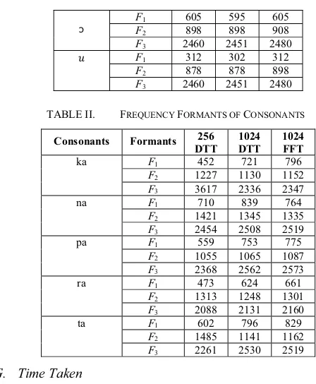
The comparison of the frequency formants using 256 DTT, 1024 DTT and 1024 FFT for five vowels and five consonant are shown in Table I and Table II.
TABLE I. FREQUENCY FORMANTS OF VOWELS
Vowels Formants 256
DTT 1024 DTT
1024 FFT
݅ FF1 2 2421 2265 2265 292 292 312
F3 3300 3300 3349
ߝ FF1 2 1777 1777 1796 546 546 546
F3 2441 2451 2470
॔ FF1 2 1093 1103 1113 703 703 712
F3 2441 2451 2480
˂
F1 605 595 605
F2 898 898 908
F3 2460 2451 2480
ݑ F1 312 302 312
F2 878 878 898
F3 2460 2451 2480
TABLE II. FREQUENCY FORMANTS OF CONSONANTS
Consonants Formants 256
DTT 1024 DTT
1024 FFT
ka F1 452 721 796
F2 1227 1130 1152
F3 3617 2336 2347
na F1 710 839 764
F2 1421 1345 1335
F3 2454 2508 2519
pa F1 559 753 775
F2 1055 1065 1087
F3 2368 2562 2573
ra F1 473 624 661
F2 1313 1248 1301
F3 2088 2131 2160
ta F1 602 796 829
F2 1485 1141 1162
F3 2261 2530 2519
G. Time Taken
The time taken of speech recognition performance using DTT and FFT is shown in Table III and Table IV.
TABLE III. TIME TAKEN OF SPEECH RECOGNITION PERFORMANCE USING DTT AND FFT
Vowels DTT FFT
256 1024 1024
݅ 0.577231 sec 0.982382 sec 0.648941 sec ߝ 0.584104 sec 0.993814 sec 0.643500 sec ॔ 0.589120 sec 0.963208 sec 0.738364 sec ˂ 0.574317 sec 0.953711 sec 0.662206 sec ݑ 0.579469 sec 0.978917 sec 0.703741 sec
TABLE IV. TIME TAKEN OF SPEECH RECOGNITION PERFORMANCE USING DTT AND FFT
Consonants DTT FFT
256 1024 1024
ka 0.589891 sec 0.991753 sec 0.731936 sec na 0.576941 sec 0.985201 sec 0.652519 sec pa 0.572490 sec 0.948586 sec 0.649752 sec ra 0.588199 sec 0.969955 sec 0.732650 sec ta 0.584613 sec 0.984997 sec 0.662382 sec
IV. EXPERIMENTS
The frequency formants of speech recognition using 256 DTT, 1024 DTT and 1024 FFT are analyzed for five vowels and five consonants. According to Table I and Table II, the experiment result shows that the peaks of first frequency formant (F1), second frequency formant (F2) and third
frequency formant (F3) using 256 DTT, 1024 DTT and 1024
The experiment result as presented in Table III and Table IV shows speech recognition performance using 256 DTT produces minimum time taken than 1024 DTT and 1024 FFT to recognize five vowels and five consonants. The time taken of speech recognition using 256 DTT produces faster computation than 1024 DTT, because the 256 DTT required smaller matrix computation and simply computationally field in transformation domain.
V. COMPARATIVE ANALYSIS
The speech recognition using 256 DTT, 1024 DTT and 1024 FFT have been compared. The power spectral density of vowel ‘O’ and consonant ‘RA’ using DTT in the Fig. 4 and Fig. 5 show that the power spectrum is lower than of FFT as presented in Fig. 6 and Fig. 7. Based on the experiments as presented in the Fig. 8, Fig. 9 and Fig. 10, Fig. 11, the peaks of first frequency formant (F1), second
frequency formant (F2) and third frequency formant (F3)
using FFT and DTT respectively to be appear identically similar. According to observation as presented in the Fig. 12, frequency formant of vowel ‘O’ in sixteen frames show identically similar output among each frame. The first formant in frame sixteen is not detected. Then, the second formant within the first and sixth frames is not appearing temporarily well captured. Then, frequency formants of consonant ‘RA’ as shown in Fig. 13 show that the second formant within fifth and seventh frame is not detected.
VI. CONCLUSION
FFT on speech recognition is a popular transformation method over the last decades. Alternatively, DTT is proposed here instead of the popular FFT. In previous research, speech recognition using 1024 DTT has been done. In this paper, the simplified matrix on 256 DTT is proposed to produces a simpler and more computationally efficient than 1024 DTT on speech recognition. 256 DTT consumes smaller matrix which can be efficiently computed on rational domain compared to the popular 1024 FFT on complex field. The preliminary experimental results show that the peaks of first frequency formant (F1), second
frequency formant (F2) and third frequency formant (F3)
using 256 DTT give identically similar output with 1024 DTT and 1024 FFT in terms of speech recognition. Speech recognition using 256 DTT scheme should perform well to recognize vowels and consonants. It can be the next candidate in speech recognition.
REFERENCES
[1] J.A. Vite-Frias, Rd.J. Romero-Troncoso and A. Ordaz-Moreno, “VHDL Core for 1024-point radix-4 FFT Computation,”
International Conference on Reconfigurable Computing and FPGAs,
Sep. 2005, pp. 20-24.
[2] R. Mukundan, “Improving Image Reconstruction Accuracy Using Discrete Orthonormal Moments,” Proceedings of International
Conference On Imaging Systems, Science and Technology, June
2003, pp. 287-293.
[3] R. Mukundan, S.H. Ong and P.A. Lee, “Image Analysis by Tchebichef Moments,” IEEE Transactions on Image Processing, Vol. 10, No. 9, Sep. 2001, pp. 1357–1364.
[4] F. Ernawan, N. A. Abu and N. Suryana, “Spectrum Analysis of Speech Recognition via Discrete Tchebichef Transform,” Proceedings of International Conference on Graphic and Image
Processing (ICGIP 2011), SPIE, Vol. 8285 No. 1, Oct. 2011.
[5] F. Ernawan, N.A. Abu and N. Suryana, “The Efficient Discrete Tchebichef Transform for Spectrum Analysis of Speech Recognition,” Proceedings 3rd International Conference on Machine
Learning and Computing, Vol. 4, Feb. 2011, pp. 50-54.
[6] F. Ernawan and N.A. Abu “Efficient Discrete Tchebichef on Spectrum Analysis of Speech Recognition,” International Journal of
Machine Learning and Computing, Vol. 1, No. 1, Apr. 2011, pp. 1-6.
[7] C.-H. Teh and R.T. Chin, “On Image Analysis by the Methods of Moments,” IEEE Transactions on Pattern Analysis Machine Intelligence, Vol. 10, No. 4, July 1988, pp. 496-513.
[8] N.A. Abu, W.S. Lang and S. Sahib, “Image Super-Resolution via Discrete Tchebichef Moment,” Proceedings of International Conference on Computer Technology and Development (ICCTD
2009), Vol. 2, Nov. 2009, pp. 315–319.
[9] R. Mukundan, “Some Computational Aspects of Discrete Orthonormal Moments,” IEEE Transactions on Image Processing, Vol. 13, No. 8, Aug. 2004, pp. 1055-1059.
[10] N.A. Abu, N. Suryana and R. Mukundan, “Perfect Image Reconstruction Using Discrete Orthogonal Moments,” Proceedings of
The 4th IASTED International Conference on Visualization, Imaging,
and Image Processing (VIIP2004), Sep. 2004, pp. 903-907.
[11] N.A. Abu, W.S. Lang and S. Sahib, “Image Projection Over the Edge,” 2nd International Conference on Computer and Network
Technology (ICCNT 2010), Apr. 2010, pp. 344-348.
[12] W.S. Lang, N.A. Abu and H. Rahmalan, “Fast 4x4 Tchebichef Moment Image Compression,” Proceedings International Conference
of Soft Computing and Pattern Recognition (SoCPaR 2009), Dec.
2009, pp. 295ԟ300.
[13] N.A. Abu, W.S. Lang, N. Suryana and R. Mukundan, “An Efficient Compact Tchebichef Moment for Image Compression,” 10th
International Conference on Information Science, Signal Processing
and their Applications (ISSPA 2010), May 2010, pp. 448-451.
[14] J. Hillenbrand, L.A. Getty, M.J. Clark, and K. Wheeler, “Acoustic Characteristic of American English Vowels,” Journal of the
Acoustical Society of America, Vol. 97, No. 5, May 1995, pp.
3099-3111.
[15] J.H. Esling and G.N. O'Grady, “The International Phonetic Alphabet,” Linguistics Phonetics Research, Department of Linguistics, University of Victoria, Canada, 1996.
[16] G.E. Peterson, and H.L. Barney, “Control Methods Used in a Study of the Vowels,” Journal of the Acoustical Society of America, Vol. 24, No. 2, Mar. 1952, pp. 175-184.
[17] A.H. Khandoker, C.K. Karmakar, and M. Palaniswami, “Power Spectral Analysis for Identifying the Onset and Termination of Obstructive Sleep Apnoea Events in ECG Recordings,” Proceeding
of The 5th International Conference on Electrical and Computer
Engineering (ICECE 2008), Dec. 2008, pp. 096-100.
[18] C. Li and S.V. Andersen, “Blind Identification of Non-Gaussian Autoregressive models for Efficient Analysis of Speech Signal,”
International Conference on Acoustic, Speech and Signal Processing,
Vol. 1, No. 1, July 2006, pp. 1205-1208.
[19] S. Ganapathy, P. Motlicek and H. Hermansky, “Autoregressive Models of Amplitude Modulations in Audio Compression,” IEEE
Transactions on Audio, Speech and Language Processing, Vol. 18,
No. 6, Aug. 2010, pp. 1624-1631.