Nuclear Theory authors titles recent submissions

arXiv:1707.02818v2 [hep-th] 12 Sep 2017

Delocalized SYZ Mirrors and Confronting Top-Down SU(3)-Structure Holographic Meson Masses at Finite g and Nc with P(article) D(ata) G(roup) Values

Vikas Yadav(a)1_{, Aalok Misra}(a),(b)2 _{and Karunava Sil}(a)3

(a) Department of Physics, Indian Institute of Technology, Roorkee - 247 667, Uttarakhand, India (b) Physics Department, McGill University, 3600 University St, Montr´eal, QC H3A 2T8, Canada

Abstract

Meson spectroscopy at finite gauge coupling - whereat any perturbative QCD computation would break down - and finite number of colors, from a top-down holographic string model, has thus far been entirely missing in the literature. This paper fills in this gap. Using the delocalized type IIA SYZ mirror (with SU(3) structure) of the holographic type IIB dual of large-N thermal QCD of [1] as constructed in [2] at finite coupling and number of colors (Nc= Number ofD5(D 5)-branes wrapping a vanishing two-cycle in the top-down holographic construct of [1] =_O(1) in the IR in the MQGP limit of [2] at the end of a Seiberg duality cascade), we obtain analytical (not just numerical) expressions for the vector and scalar meson spectra and compare our results with previous calculations of [3], [4], and obtain a closer match with the Particle Data Group (PDG) results [5]. Through explicit computations, we verify that the vector and scalar meson spectra obtained by the gravity dual with a black hole for all temperatures (small and large) are nearly isospectral with the spectra obtained by a thermal gravity dual valid for only low temperatures; the isospectrality is much closer for vector mesons than scalar mesons. The black hole gravity dual (with a horizon radius smaller than the deconfinement scale) also provides the expected large-N

suppressed decrease in vector meson mass with increase of temperature.

1

Introduction

The AdS/CFT [6] correspondence and its non-conformal generalizations, conjecture the equivalence between string theory on a ten dimensional space-time and gauge theory living on the boundary of space-time. A generalization of the AdS/CFT correspondence is necessary to explore more realistic theories (less supersymmetric and non conformal) such as QCD. The original AdS/CFT conjecture [6] proposed a duality between maximally supersymmetricN = 4 SU(N) SYM gauge theory and type IIB supergravity onAdS5×S5in the low enegry limit. Different generalized versions of the AdS/CFT

have thus far been proposed to study non-supersymmetric field theories. One way of constructing gauge theories with less supersymmetry is to consider stacks of Dp branes at the singular tip of a Calabi-Yau cone. In this paper we use a large N top down holographic dual of QCD[1] to obtain the meson spectrum from type IIA perspective. Embedding of additional D-branes(flavor branes) in the near-horizon limit gives rise to a modification of the original AdS/CFT correspondence which involves field theory degrees of freedom that transform in the fundamentalrepresentation of the gauge group. This is useful for describing field theories like QCD, where quark fields transform in the fundamental representation. Mesons operator or a gauge invariant bilinear operator corresponds to the bound state of anti-fundamental and fundamental field.

In the past decade, (glueballs and) mesons have been studied extensively to gain new insight into the non-perturbative regime of QCD. Various holographic setups such as soft-wall model, hard wall model, modified soft wall model, etc. have been used to obtain the glueballs’ and mesons’ spectra and obtain interaction between them. In the following two paragraphs a brief summary of the work is given that has been done in past decades.

Most of existing literature on holographic meson spectroscopy is of the bottom-up variety based often on soft/hard wall AdS/QCD models. Here is a short summary of some of the relevant works. Soft-wall holographic QCD model was used in [7] and [8] to obtain spectrum and decay constants for 1−+ hybrid mesons and to study the scalar glueballs and scalar mesons at T 6= 0 respectively. In [7] no states with exotic quantum numbers were observed in the heavy quark sector. Comparison of the computed mass with the experimental mass of the 1−+ _{candidates π}

1(1400), π1(1600) and π1(2015),

favoredπ1(1400) as the lightest hybrid state. In [9] an IR-improved soft-wall AdS/QCD model in good

agreement with linear confinement and chiral symmetry breaking was constructed to study the mesonic spectrum. The model was constructed to rectify inconsistencies associated with both simple soft-wall and hard-wall models. The hard-wall model gave a good realization for the chiral symmetry breaking, but the mass spectra obtained for the excited mesons didn’t match up with the experimental data well. The soft-wall model with a quadratic dilaton background field showed the Regge behaviour for excited vector mesons but chiral symmetry breaking phenomena cannot be realized consistently in the simple soft-wall AdS/QCD model. A hard wall holographic model of QCD was used in [10], [11] and [12] to analyze the mesons. In [13] a two-flavor quenched dynamical holographic QCD(hQCD) model was constructed in the graviton-dilaton framework by adding two light flavors. In [3] the mesonic spectrum was obtained for aD4/D8(₋D8)-brane configuration in type IIA string theory; in [14] massive excited states in the open string spectrum were used to obtain the spectrum for higher spin mesons J _≥2. NLO terms were obtained by taking into account the effect of the curved background perturbatively which led to corrections in formula J = α0+α′M2. The results obtained for the meson spectrum

were compared with the experimental data to identify a2(1320), b1(1235), π(1300), a0(1450) etc. first

include quark in the fundamental representations.

To our knowledge, the only top-down holographic dual of large-N thermal QCD which is IR confining, UV conformal and UV-complete (e.g. the holographic Sakai-Sugimoto model [3] does not address the UV) with fundamental quarks is the one given in [1] involvingN D3-branes,M D5/(D5) branes wrapping a vanishing two-cycle andNf D7(D7) flavor-branes in a warped resolved conifold at finite temperature in the brane picture (and M D5-branes andD7(D7)-branes with a black-hole and fluxes in a resolved warped deformed conifold gravitational dual). In [4], the authors (some also part of [1]) obtained the vector and scalar mesonic spectra by taking a single T-dual of the holographic type IIB background of [1]. Comparison of the (pseudo-)vector mesons with PDG results, provided a reasonable agreement. One of the main objectives of our work is to see if by taking a mirror of the type IIB background of [1] via delocalized Strominger-Yau-Zaslow’s triple-T-duality prescription - a new tool in this field - at finite gauge coupling and with finite number of colors - a new limit and one which is closest to realistic strongly coupled thermal QCD - one can obtain a better agreement between the mesonic spectra so obtained and PDG results than previously obtained in [3] and [4], and in the process gain new insights into a holographic understanding of thermal QCD.

In [16], we initiated top-down G-structure holographic large-N thermal QCD phenomenology at finite gauge coupling and finite number of colors, in particular from the vantage point of the M theory uplift of the delocalized SYZ type IIA mirror of the top-down UV complete holographic dual of large-N thermal QCD of [1], as constructed in [2]. We calculated up to (N)LO in N, masses of 0++,0−−,0−+,1++ and 2++ glueballs, and found very good agreement with some of the lattice results on the same. In this paper, we continue exploring top-down G-structure holographic large-N

thermal QCD phenomenology at finite gauge coupling by evaluating the spectra of (pseudo-)vector and (pseudo-)scalar mesons, and in particular comparing their ratios for both types with P(artcile) D(ata) G(roup) results.

The rest of the paper is organized as follows. In Section2, via four sub-sections, we briefly review a UV-complete top-down type IIB holographic dual of large-N thermal QCD (subsection2.1) as given in [1] and its M theory uplift in the ‘MQGP limit’ as worked out in [2] (sub-section 2.2); sub-section

2.3 has a discussion on the construction in [2] of the delocalized Strominger-Yau-Zaslow (SYZ) type IIA mirror of the aforementioned type IIB background of [1] and sub-section 2.4 has a brief review of SU(3) and G2 structures relevant to [1] (type IIB) and [2, 17] (type IIA and M theory). Section 3 is on the construction of the embedding of D6-branes via delocalized SYZ type IIA mirror of the embedding of D7-branes of type IIB. Via five sub-sections, Section 4 is on obtaining the (pseudo-)vector meson spectra in the framework of [2] at finite coupling assuming a black hole gravity dual for all temperatures, small and large. The (pseudo-)vector mesons correspond to gauge fluctuations about a background gauge field along the world volume of the D6 branes. Unlike [4], the gravity dual involves a black-hole (rh 6= 0) and consequently, while factorizing the gauge fluctuations along

R3_×S1_{-radial direction into fluctuations along} R3_×S1 _{and eigenmode fluctuations along the radial}

direction, there are two types of eigenmodes along the radial direction - one denoted by α{ni}(Z) which is coupled to gauge fluctuations along the space-like R3 _{and the other denoted by α}{_n0}_{(Z) which is}

coupled to the compact time-like S1 _{(metric along which includes the black-hole function). After}

obtaining the EOMs for α{ni} and α{n0}, the following is the outline of what is done in subsections

Finally, using the WKB quantization prescription, the vector meson spectrum corresponding to the

α{ni} eigenmodes was worked out (in the small and large mass-limits) in 4.4, and that corresponding to the α{n0} eigenmodes (in the small and large mass-limits) in 4.5. In Section5, we obtain the scalar meson spectrum by considering fluctuations of the D6-branes orthogonal to their world-volume in the absence of any background gauge fields in a black hole background for all temperatures, small and large. In the same vein as vector meson spectroscopy, after obtaining the EOM for the radial eigenfunction mode, the following is an outline of what is done in section 5, devoted to scalar meson spectroscopy. First, in 5.1, assuming an IR-valued scalar meson spectrum, the same is obtained by solving the EOMs near the horizon. Next, by converting the EOMs to a Schr¨odinger-like EOMs, the scalar meson spectrum is worked out for in 5.2 (in the IR limit in5.2.1 and the UV limit in5.2.2). Finally, using the WKB quantization prescription, the scalar meson spectrum was worked out (in the small and large mass-limits) in 5.3. In Section 6, we obtain the (pseudo-)vector meson spectrum in

6.1(and the three sub-sub-sections therein) and (pseudo-)scalar meson spectrum in6.2(and the three sub-sub-sections therein) using a thermal background, and hence verify that the mesonic spectra of Sections 4 and 5 are nearly isospectral with 6. Section 7 has a discussion on the new insights and results obtained in this work and some future directions. There are three supplementary appendices.

2

Background: A Top-Down Type IIB Holographic Large-

N

Ther-mal QCD and its M-Theory Uplift in the ‘MQGP’ Limit

Via four sub-sections, in this section, we will:

• provide a short review of the type IIB background of [1], a UV complete holographic dual of large-N thermal QCD, in subsection2.1,

• discuss the ’MQGP’ limit of [2] and the motivation for considering this limit in subsection 2.2,

• briefly review issues as discussed in [2], [18], [17] and [19], pertaining to construction of delocalized S(trominger) Y(au) Z(aslow) mirror and approximate supersymmetry, in subsection2.3,

• briefly review the new results of [17] and [19] pertaining to construction of explicit SU(3) and

G2 structures respectively of type IIB/IIA, and M-theory uplift,

2.1 Type IIB Dual of Large-N Thermal QCD

ten-dimensional geometry is given by a resolved warped deformed conifold. In the gravity dual D 3-branes and the D5-branes are replaced by fluxes in the IR. The finite temperature resolves 4 and IR confinement deforms the conifold. Back-reactions are included in the warp factor and fluxes.

One hasSU(N+M)×SU(N+M) color gauge group andSU(Nf)×SU(Nf) flavor gauge group, in the UV. It is expected that there will be a partial Higgsing ofSU(N+M)_×SU(N+M) toSU(N+

M)_×SU(N) atr=_RD5/D5 [21]. The two gauge couplings,g_SU(N+M)andg_SU(N)flow logarithmically and oppositely in the IR: 4π2

1

g2 SU(N+M)

+_g21 SU(N)

eφ∼π; 4π2

1

g2

SU(N+M) −

1

g2 SU(N)

eφ∼ 1 2πα′

R

S2B2

.Had it not been forR_S2B2, in the UV, one could have setg2_SU(M+N)=g_SU2 _(N)=g_{Y M}2 ∼gs≡constant (implying conformality) which is the reason for inclusion of M D5-branes at the common boundary of the UV-IR interpolating and the UV regions, to annul this contribution. In fact, the running also receives a contribution from the Nf flavor D7-branes which needs to be annulled viaNf D7-branes. Under an NVSZ RG flow, the gauge coupling g_SU(N+M) - having a larger rank - flows towards strong coupling and the SU(N) gauge coupling flows towards weak coupling. Upon application of Seiberg duality,SU(N+M)strong

Seiberg Dual

−→ SU(N₋(M₋Nf))weak in the IR; assuming after duality cascade,

N decreases to 0 and there is a finiteM, one will be left withSU(M) gauge theory with Nf flavors that confines in the IR - the finite temperature version of the same is what was looked at by [1].

So, in the IR, at the end of the duality cascade, number of colorsNc is identified with M, which in the ‘MQGP limit’ can be tuned to equal 3. One can identify Nc with Neff(r) +Meff(r), where

Neff(r) =

R

Base of Resolved Warped Deformed ConifoldF5 and Meff =

R

S3F˜3 (the S3 being dual to eψ ∧ (sinθ1dθ1∧dφ1−B1sinθ2∧dφ2), wherein B1 is an asymmetry factor defined in [1], andeψ ≡dψ+ cosθ1 dφ1+ cosθ2 dφ2) where ˜F3(≡F3−τ H3)∝M(r)≡ 1

1+eα

r−R_D5/D5

, α≫1 [22]. The number of

colors Nc varies betweenM in the deep IR and a large value [even in the MQGP limit of (10) (for a large value ofN)] in the UV. Hence, at very low energies, the number of colorsNccan be approximated by M, which in the MQGP limit is taken to be finite and can hence be taken to be equal to three. In [1], the effective number of D3-branes,D5-branes wrapping the vanishing two-cycle and the flavor

D7-branes, denoted respectively by Neff(r),Meff(r) and Nfeff(r), are given as:

Neff(r) =N

"

1 +3gsM

2 eff

2πN logr+

3gsNfeff 2π (logr)

2

!# ,

Meff(r) =M+

3gsNfM

2π logr+ X

m≥1

X

n≥1

N_fmMnfmn(r),

N_feff(r) =Nf +

X

m≥1

X

n≥0

N_fmMngmn(r). (1)

It was argued in [17] that the length scale of the OKS-BH metric in the IR after Seiberg-duality

4_{The non-zero resolution parameter ‘a’ is also there to introduce a separationR}

D5/D5between theD5 andD5 branes,

cascading away almost the whole of Neff, will be given by:

which implies that in the IR, relative to KS, there is a color-flavor enhancement of the length scale in the OKS-BH metric. Hence, in the IR, even for N_cIR = M = 3 and Nf = 2 (light flavors) upon inclusion of n, m >1 terms in Meff and N_feff in (1), LOKS−BH≫LKS(∼LPlanck) in the MQGP limit

involving gs ∼

<1, implying that the stringy corrections are suppressed and one can trust supergravity calculations. Further, the global flavor group SU(Nf)×SU(Nf), is broken in the IR to SU(Nf) as the IR has only Nf D7-branes.

Hence, the type IIB model of [1] makes it an ideal holographic dual of thermal QCD because, it is UV conformal and IR confining with required chiral symmetry breaking in the IR. The quarks present in the theory transform in the fundamental representation, plus theory is defined for full range of temperature both low and high.

(d) Supergravity solution on resolved warped deformed conifold

The metric in the gravity dual of the resolved warped deformed conifold withgi’s: g1,2(r, θ1, θ2) =

The compact five dimensional metric in (3), is given as:

d_M2₅ =h1(dψ+ cos θ1 dφ1+ cos θ2 dφ2)2+h2(dθ12+ sin2θ1 dφ21) +h4(h3dθ22+ sin2θ2 dφ22)

+h5[ cosψ(dθ1dθ2−sin θ1sinθ2dφ1dφ2) + sinψ(sin θ1 dθ2dφ1+ sin θ2 dθ1dφ2)], (4)

wherein we will assume r ≫ a, h5 ∼ (deformation parameter)

2

r3 ≪ 1 for r ≫ (deformation parameter) 2 3.

The hi’s appearing in internal metric up to linear order depend on gs, M, Nf are given as below:

h1 =

IR) = R_{warped squashed S}2_(a)×S3_(ǫ)F5(r ∈ IR) ≪ M =

R

S3_(ǫ)F3(r ∈ IR); we have a confining SU(M)

gauge theory in the IR.

The warp factor that includes the back-reaction, in the IR is given as:

h= L

where, in principle,Meff/Nfeff are not necessarily the same asM/Nf; we however will assume that up to OgsM2

N

, they are. Proper UV behavior requires [21]:

h= L

+_Odeformation parameter_r3 2

+O(deformation parameter)_r3 2

. As in the UV, (deformation parameter)_r3 2 ≪

(resolution parameter)2

r2 , we will assume the same three-form fluxes for h5 6= 0. With RD5/D5 denoting

the boundary common to the UV-IR interpolating region and the UV region, ˜Flmn, Hlmn = 0 for

r _{≥ RD5/D5} is required to ensure conformality in the UV. Near the θ1 = θ2 = 0-branch,

assum-the MQGP limit. This mimics addition of D5-branes in [1] to ensure cancellation of ˜F3.

2.2 The ‘MQGP Limit’

In [2], we had considered the following two limits:

(i)weak(gs)coupling−large t′Hooft coupling limit :

gs ≪1, gsNf ≪1,

gsM2

N ≪1, gsM ≫1, gsN ≫1

effected by :gs∼ǫd, M ∼(O(1)ǫ)−

3d

2 _{, N} ∼₍O_(1)ǫ)−19d_{, ǫ}≪_{1, d >0 (9)}

(the limit in the first line though not its realization in the second line, considered in [1]);

(ii)MQGP limit : gsM

2

N ≪1, gsN ≫1,finitegs, M

effected by :gs∼ǫd, M ∼(O(1)ǫ)−

3d

2 , N ∼(O(1)ǫ)−39d, ǫ.1, d >0. (10)

The motivation for considering the MQGP limit which was discussed in detail in [17] is:

1. Unlike the AdS/CFT limit wherein gYM → 0, N → ∞ such that gYM2 N is large, for strongly

coupled thermal systems like sQGP, what is relevant is gYM ∼ O(1) and Nc = 3. From the discussion in the previous paragraphs one sees that in the IR after the Seiberg duality cascade, effectively Nc =M which in the MQGP limit of (10) can be tuned to 3. Further, in the same limit, the string coupling gs ∼< 1. The finiteness of the string coupling necessitates addressing the same from an M theory perspective. This is the reason for coining: ‘MQGP limit’. In fact this is the reason why one is required to first construct a type IIA mirror, which was done in [2] `

a la delocalized Strominger-Yau-Zaslow mirror prescription, and then take its M-theory uplift. 2. The second set of reasons for looking at the MQGP limit of (10) is calculational simplification

in supergravityy:

• In the UV-IR interpolating region and the UV, (Meff, Neff, N_feff) MQGP

≈ (M, N, Nf)

• Asymmetry FactorsAi, Bj(in three-form fluxes) M QGP

→ 1 in the UV-IR interpolating region and the UV.

• Simplification of ten-dimensional warp factor and non-extremality function in MQGP limit

2.3 Approximate Supersymmetry, Construction of the Delocalized SYZ IIA Mir-ror and Its M-Theory Uplift in the MQGP Limit

To implement the quantum mirror symmetry a la SYZ [23], one needs a special Lagrangian (sLag)T3

fibered over a large base. Defining delocalized T-duality coordinates, (φ1, φ2, ψ)→ (x, y, z) valued in

T3(x, y, z) [2]:

x =ph2h

1

4sinhθ₁ihriφ₁, y=ph₄h14sinhθ₂ihriφ₂, z =ph₁hrih14ψ, (11)

using the results of [24] it was shown in [18, 19] that the following conditions are satisfied:

i∗J|RC/DC≈0,

ℑm(i∗Ω)|RC/DC≈0,

ℜe(i∗Ω)|RC/DC ∼volume form T3(x, y, z)

for theT2-invariant sLag of [24] for a deformed conifold P4_i=1z_i2= 1:

K′(r2)ℑm(z1z¯2) =c1, K′(r2)ℑm(z3¯z4) =c2,ℑm(z12+z22) =c3, (13)

and the T2_{-invariant sLag of [24] of a resolved conifold:}

K′

2 |x|

2_{− |y|}2_{+ 4a}2 |λ2|2

|λ1|2+|λ2|2

=c1,

K′

2 |v|

2_{− |u|}2_{+ 4a}2 |λ2|2

|λ1|2+|λ2|2

=c2,

ℑm(xy) =c3, (14)

wherein one uses the following complex structure for a resolved conifold [25]:

x = 9a2r4+r61/4ei/2(ψ−φ1−φ2) _sinθ1

2 sin

θ2

2

y = 9a2r4+r61/4ei/2(ψ+φ1+φ2) _cosθ1

2 cos

θ2

2

u = 9a2r4+r61/4ei/2(ψ+φ1−φ2) _cosθ1

2 sin

θ2

2

v = 9a2r4+r61/4ei/2(ψ−φ1+φ2) _sinθ1

2 cos

θ2

2 

  

x y u v

   =

1

√

2    

1 ₋i 0 0

1 i 0 0

0 0 −i 1

0 0 ₋i ₋1

  

. (15)

In (14), [λ1 : λ2] are the homogeneous coordinates of the blown-up CP1 = S2; _λλ2₁ = ₋x_u = ₋v_y =

−e−iφ1_tanθ1

2. In (14),γ(r2)≡r2K′(r2) =−2a2+4a4N−

1

3(r2)+N13(r2), whereN(r2)≡ 1

2

r4−16a6+√r8_−32a6_r4

Hence, if the resolved warped deformed conifold is predominantly either resolved or deformed, the local

T3 _{of (11) is the required sLag to effect SYZ mirror construction.}

Interestingly, in the ‘delocalized limit’ [26]ψ=hψi, under the coordinate transformation:

sinθ2dφ2

dθ2

→

cos_hψ_i sin_hψ_i

−sin_hψ_i cos_hψ_i

sinθ2dφ2

dθ2

, (16)

andψ_→ψ₋cos_hθ¯2iφ2+coshθ2iφ2−tanhψilnsin ¯θ2, theh5term becomesh5[dθ1dθ2−sinθ1sinθ2dφ1dφ2],

eψ →eψ, i.e., one introduces an local (not global) isometry alongψin addition to the isometries along

φ1,2.

To enable use of SYZ-mirror duality via three T dualities, remembering that SYZ mirror symmetry is in fact a quantum mirror symmetry, one also needs to ensure a large base (implying large complex structures of the aforementioned two two-tori) of theT3_{(x, y, z) fibration, ensuring the disc instantons’}

contribution is very small [23]. This is effected via [27]:

dψ →dψ+f1(θ1) cosθ1dθ1+f2(θ2) cosθ2dθ2,

for appropriately chosen large values of f1,2(θ1,2) = ±cotθ1,2 [17]. The three-form fluxes remain

invariant. The guiding principle behind choosing such large values of f1,2(θ1,2), as given in [2], is

that one requires the metric obtained after SYZ-mirror transformation applied to the non-K¨ahler resolved warped deformed conifold to be like a non-K¨ahler warped resolved conifold at least locally. For completenes, we summarize the Buscher triple-T duality rules [28],[2] in appendix A.

A single T-duality along a direction orthogonal to the D3-brane world volume, e.g., z of (11), yields D4 branes straddling a pair ofN S5-branes consisting of world-volume coordinates (θ1, x) and

(θ2, y). Further, T-dualizing along x and theny would yield a Taub-NUT space from each of the two

N S5-branes [29]. The D7-branes yield D6-branes which get uplifted to Kaluza-Klein monopoles in M-theory [30] which too involve Taub-NUT spaces. Globally, probably the eleven-dimensional uplift would involve a seven-fold ofG2-structure, analogous to the uplift ofD5-branes wrapping a two-cycle

in a resolved warped conifold [31]. We obtained a local G2 structure in [17], which is summarized in 2.4.

2.4 G-Structures

In this sub-section, we give a quick overview of G=SU(3), G2-structures and how the same appear

in the holographic type IIB dual of [1], its delocalized type IIA SYZ mirror and its M-theory uplift constructed in [2].

Any metric-compatible connection can be written in terms of the Levi-Civita connection and the contorsion tensorκ ([32] and references therein). Metric compatibility requiresκ∈Λ1⊗Λ2, Λnbeing the space of n-forms. Alternatively, in d complex dimensions, since Λ2 ∼= so(d), κ also be thought of as Λ1_{⊗so(d). Given the existence of a G-structure, one can decompose so(d) into a part in the}

Lie algebra g of G ⊂ SO(d) and its orthogonal complement g⊥ = so(d)/g. The contorsion κ splits accordingly into κ = κ0 +κg, where κ0 - the intrinsinc torsion - is the part in Λ1 _⊗g⊥. One can decompose κ0 _{into irreducible G representations providing a classification of G-structures in terms}

of which representations appear in the decomposition. Let us consider the decomposition of T0 in the case of SU(3)-structure. The relevant representations are Λ1 ∼ 3⊕¯3, g ∼ 8, g⊥ ∼ 1⊕3⊕¯3.

Thus the intrinsic torsion, an element of Λ1 _⊕su(3)⊥_{, can be decomposed into the following SU(3)} representations [32] :

Λ1_⊗su(3)⊥= (3_⊕¯3)_⊗(1_⊕3_⊕3)¯

= (1_⊕1)_⊕(8_⊕8)_⊕(6_⊕¯6)_⊕(3_⊕¯3)_⊕(3_⊕¯3)′ _≡W1⊕W2⊕W3⊕W4⊕W5. (18)

The SU(3) structure torsion classes [33] can be defined in terms of J, Ω, dJ, dΩ and the contraction operator y: Λk_T⋆_⊗Λn_T⋆_→Λn−k_T⋆_{. The torsion classes are then defined in the following way:}

• W1↔[dJ](3,0), given by real numbersW1=W1++W1−withdΩ+∧J = Ω+∧dJ =W1+J∧J∧J

and dΩ_−∧J = Ω_−∧dJ =W₁−J _∧J_∧J;

• W2↔[dΩ](2₀ ,2) : (dΩ+)(2,2) =W₁+J ∧J+W₂+∧J and (dΩ−)(2,2)=W1−J∧J+W2−∧J;

• W3↔[dJ](20,1) is defined asW3 =dJ(2,1)−[J∧W4](2,1);

• W4= 1₂JydJ;

In [18], it was shown that the five SU(3) structure torsion classes, in the MQGP limit, satisfied (schematically):

T_SUIIB₍₃₎ ∈W1⊕W2⊕W3⊕W4⊕W5∼

e−3τ

√

gsN ⊕ (gsN)

1

4 e−3τ⊕pg_sN e−3τ⊕ −2

3 ⊕ − 1 2

(19)

(r_∼eτ3), such that

2 3W

¯ 3

5 =W

¯ 3

4 (20)

in the UV-IR interpolating region/UV, implying a Klebanov-Strassler-like supersymmetry [34]. Locally aroundθ1∼ 1

N15, θ2 ∼

1

N103 , the type IIA torsion classes of the delocalized SYZ type IIA mirror metric

were shown in [17] to be:

T_SUIIA₍₃₎ ∈ W2⊕W3⊕W4⊕W5∼γ2g−

1 4

s N

3 10 ⊕g−

1 4

s N−

1 20 ⊕g−

1 4

s N

3 10 ⊕g−

1 4

s N

3

10 ≈γW₂⊕W₄⊕W₅

fine tuning:γ≈0

−→ ≈W4⊕W5. (21)

Further,

W4∼ ℜeW5 (22)

indicative of supersymmetry after constructing the delocalized SYZ mirror.

The mirror type IIA metric after performing three T-dualities, first along x, then along y and finally along z, utilizing the results of [26] was worked out in [2]. The type IIA metric components were worked out in [2].

Apart from quantifying the departure fromSU(3) holonomy due to intrinsic contorsion supplied by the NS-NS three-form H, via the evaluation of theSU(3) structure torsion classes, to our knowledge for the first time in the context of holographic thermal QCD at finite gauge coupling and for finite number of colors [in fact for Nc = 3 in the IR]in [17]:

(i) the existence of approximate supersymmetry of the type IIB holographic dual of [1] in the MQGP limit near the coordinate branch θ1 = θ2 = 0 was demonstrated, which apart from the existence of

a special Lagrangian three-cycle (as shown in [18, 17]) is essential for construction of the local SYZ type IIA mirror;

(ii) it was demonstrated that the large-N suppression of the deviation of the type IIB resolved warped deformed conifold from being a complex manifold, is lost on being duality-chased to type IIA - it was also shown that one further fine tuning γ2 = 0 in W2IIA can ensure that the local type IIA mirror is

complex;

(iii) for the local type IIASU(3) mirror, the possibility of surviving approximate supersymmetry was demonstrated which is essential from the point of view of the end result of application of the SYZ mirror prescription.

We can get a one-form type IIA potential from the triple T-dual (along x, y, z) of the type IIB

F1,3,5 in [2] and using which the following D= 11 metric was obtained in [2] (u≡ r_rh):

ds2₁₁=e−2φIIA3 g_ttdt2+gR3 dx2+dy2+dZ2+g_uudu2+ds2_IIA(θ_1,2, φ_1,2, ψ)

+e4φIIA3

dx11+AF1 +AF3+AF5

2

≡ Black M3₋Brane +_O

gsM2logN

N

(gsNf)

.

Let us now briefly discussG2structure. We will be following [35, 37, 36]. IfV is a seven-dimensional

real vector space, then a three-formϕis said to be positive if it lies in theGL(7,R_{) orbit ofϕ0, where}

ϕ0 is a three-form onR7which is preserved byG2-subgroup ofGL(7,R). The pair (ϕ, g) for a positive

3-form ϕ and corresponding metric g constitute a G2-structure. The space of p-forms are known to

decompose as following irreps of G2 [35]:

Λ1 = Λ1₇ Λ2 = Λ2_7⊕Λ2₁₄ Λ3 = Λ3₁⊕Λ3₇⊕Λ3₂₇ Λ4 = Λ4₁⊕Λ4₇⊕Λ4₂₇ Λ5 = Λ5_7⊕Λ5₁₄

Λ6 = Λ6₇ (24)

The subscripts denote the dimension of representation and components of same representation/dimensionality, are isomorphic to each other. Let M be a 7-manifold with a G2-structure (ϕ, g). Then the

compo-nents of spaces of 2-, 3-, 4-, and 5-forms are given in [35, 37]. The metricg defines a reduction of the frame bundle F to a principal SO(7)-sub-bundle of oriented orthonormal frames. Now,g also defines a Levi-Civita connection ∇on the tangent bundle T M, and hence on F. However, theG2-invariant

3-form ϕ reduces the orthonormal bundle further to a principal G2-subbundle Q. The Levi-Civita

connection can be pulled back to Q. OnQ,_∇ can be uniquely decomposed as

∇= ¯_∇+_T (25)

where ¯∇is aG2-compatible canonical connection, taking values in the sub-algebrag2 ⊂so(7), while

T is a 1-form taking values in g⊥₂ ⊂so(7); T is known as the intrinsic torsion of the G₂structure

-the obstruction to -the Levi-Civita connection being G2-compatible. Nowso(7) splits under G2 as

so(7)∼= Λ2V ∼= Λ2₇⊕Λ2₁₄. (26)

But Λ2

14∼=g2, so the orthogonal complement g⊥₂ ∼= Λ2₇ ∼=V. Hence T can be represented by a tensor Tab which lies in W ∼= V ⊗V. Now, since ϕ is G2-invariant, it is ¯∇-parallel. So, the torsion is

determined by_∇ϕ. Now, from the Lemma 2.24 of [36]:

∇ϕ_∈Λ1_7⊗Λ3₇ ∼=W. (27) Due to the isomorphism between the Λa₇=1,...,5s,_∇ϕlies in the same space asTAB and thus completely determines it. Equation (27) is equivalent to:

∇AϕBCD =TAEψEBCD (28) where TAB is the full torsion tensor. Equation (28) can be inverted to yield:

T_AM = 1

24(∇AϕBCD)ψ

M BCD_{. (29)}

The tensor T M

A , like the space W, possesses 49 components and hence fully defines ∇ϕ. In general

TAB cab be split into torsion components as

whereT1 is a function and gives the1component ofT . We also haveT7, which is a 1-form and hence

gives the 7 component, and, T14∈Λ214 gives the 14 component. Further, T27 is traceless symmetric,

and gives the27 component. Writing Ti asWi, we can split W as

W =W1⊕W7⊕W14⊕W27. (31)

From [39], we see that aG2 structure can be defined as:

ϕ0 =

1 3!fABCe

ABC _=e−φIIA

fabceabc+e−

2φIIA

3 J∧ex10, (32)

where A, B, C = 1, ...,6,10;a, b, c,= 1, ...,6 and fABC are the structure constants of the imaginary octonions. Using the same and [38]:

dϕ0 = 4W1∗7ϕ0−3W7∧ϕ0− ∗7W27

d∗7ϕ0 =−4W7∧ ∗7ϕ0−2∗7W14, (33)

theG2-structure torsion classes were worked out around θ1∼ 1

N15, θ2 ∼

1

N103 in [17] to:

TG2 ∈W

14

2 ⊕W327∼

1 (gsN)

1 4

⊕ 1

(gsN)

1 4

. (34)

Hence, the approach of the seven-fold, locally, to having a G2 holonomy (W₁G2 = W₂G2 = W₃G2 =

WG2

4 = 0) is accelerated in the MQGP limit.

As stated earlier, the global uplift to M-theory of the typeIIB background of [1] is expected to involve a seven-fold of G2 structure (not G2-holonomy due to non-zero G4). It is hence extremely

important to be able to see this, at least locally. It is in this sense that the results of [2] are of great significance as one explicitly sees, for the first time, in the context of holographic thermal QCD

at finite gauge coupling, though locally, the aforementioned G2 structure having worked out the

non-trivial G2-structure torsion classes.

3

SYZ Mirror of Ouyang Embedding

To start off our study of meson spectroscopy, we first need to understand how the flavor D6-branes are embedded in the mirror (constructed in [2]) of the resolved warped deformed conifold of [1], i.e., the delocalized SYZ mirror of the Ouyang embedding of the flavor D7-branes in [1].

One can show that the delocalised type IIA mirror metric of the resolved warped deformed conifold metric as worked out in [2], for fixed θ1 = αθ1

N15 in the (θ2, T

3_{(x, y, z))-subspace near θ}

2 = αθ2

N103 can be

written as:

ds2_IIA(θ2, T3(x, y, z)) = dθ22N

7 10 ξ_θ

2θ2 α2_θ1 α2

θ2

√

gsdθ2+ξθ2yN− 7 20g

1 4

sdy−ξθ2z

logrM Nf

αθ2

N−1320g 7 4

sdz

!

+ds2(T3(x, y, z))

N≫1

−→ ξθ2θ2 α2_θ1 α2

θ2

√

where the T3(x, y, z) metric is given by:

Interestingly, one can diagonalize the local T3 metric to:

ds2_IIA(T3(x, y, z)) = 2dx˜

in the MQGP limit):

There is an important message we must take in from (39). As one realizes from (A11) and therefore (39), BIIA _{is independent of M even up to NLO in N even thoughB}IIB _{is proportional to M. This}

will be important in obtaining the mesonic spectra in the subsequent sections and obtaining a good match with [5] without having to invoke _OgsM2

N

-corrections which the authors of [4] had to use (and set to 0.5 - and yet consider the same to ’small’ - to get a reasonable match with [5]).

The complete 10 dimensional type IIA metric in large N limit is given as:

ds2_{IIA ≈}GIIA₀₀ dx2₀+GIIA₁₁ dx2₁+GIIA₂₂ dx2₂+GIIA₃₃ dx2₃+GIIA_rr dr2+GIIA_θ1θ1dθ₁2+GIIA_θ1x˜dθ1dx˜+GθIIA1y˜dθ1dy˜

+GIIA_θ1˜zdθ1dz˜+GIIAθ2θ2dθ

2

2+ds2(T3(˜x,y,˜ z˜))

(40)

To obtain the pullback metric on the D6 branes, we choose the first branch of the Ouyang embedding where (θ1,x˜) = (0,0) and we consider the ˜z coordinate as a function of r, i.e. ˜z(r). We then use the

following:

GIIA00 =−

r4−rh4 3gsM2log(r)(−2gsNflog(αθ1αθ2) +gsNflog(N)−6gsNf+gsNflog(16)−8π)−36gs2M2Nflog2(r) + 32π2N 64π5/2√_gsN3/2_r2

GIIA11 =

r2 3gsM2log(r)(−2gsNflog(αθ1αθ2) +gsNflogN−6gsNf+gsNflog(16)−8π)−36gs2M2Nflog2(r) + 32π2N 64π5/2√_gsN3/2

GIIA22 =

r2 3gsM2log(r)(−2gsNflog(αθ1αθ2) +gsNflogN−6gsNf+gsNflog(16)−8π)−36gs2M2Nflog2(r) + 32π2N

64π5/2√_g sN3/2

GIIA₃₃ = r

2 _3g

sM2log(r)(−2gsNflog(αθ1αθ2) +gsNflogN−6gsNf+gsNflog(16)−8π)−36gs2M2Nflog2(r) + 32π2N

64π5/2√_gsN3/2

GIIArr =

√_g

sr2 6a2+r2 3gsM2log(r)(2gsNflog(αθ1αθ2)−gsNflogN+ 6gsNf−2gsNflog(4) + 8π) + 36gs2M2Nflog2(r) + 32π2N 16π3/2√_N(9a2_+r2_{) (r}4_−rh4₎

GIIAy˜y˜ =−

29√2√6₃

αN4/5−2 32/3_N

27α2 θ12α

2 θ2

GIIAθ2θ2=

√

π√gs

√

Nα2θ12 5

√

N+α2θ2

3

√

3α2 θ2

. (42)

One will assume that the embedding of theD6-brane will be given byi: Σ1,6R1,3_{, r, θ2 ∼} αθ2

N103 ,y˜

֒_→ M1,9, effected by: ˜z= ˜z(r). The pull back of the B-field along the directions of the D6-branes is given by:

δ

θ2−

αθ2 N103

i∗B=δ

θ2−

αθ2 N103

−Bθ2z˜z˜′(r)dr∧dθ2+Bθ2y˜dθ2∧dy˜+Bθ2x˜dθ2∧dx˜

,

(43)

where Bθ2x˜, Bθ2y˜, Bθ2z˜ can be read off from (117). Now, one can show that:

det (i∗(g+B)) = Σ0(r;gs, Nf, N, M) + Σ1(r;gs, Nf, M, N) ˜z′(r)

2

, (44) where the embedding functions Σ0,1(r;gs, Nf, M, N) are given in (B1).

Thus, the Euler-Lagrange equation of motion yields:

d dr

˜

z′(r) p

Σ0(r;gs, Nf, N, M) + Σ1(r;gs, Nf, N, M)(˜z′)2

!

= 0. (45)

Like [4], ˜z=constant, is a solution of (45). Alternatively, (45) is equivalent to:

˜

z′_(r)

√

Σ0(r;gs,Nf,N,M)+Σ1(r;gs,Nf,N,M)(˜z′)2 = K. Hence, the Euler-Lagrange equation for the ˜z(r) from the DBI action can be written in the following form:

z′(r)2₋ 24461180928π

19/2_α16

θ1α

8

θ2C1gs

4_KN49/5

C22−24461180928π19/2α16θ1α

8

θ2C3gs

4_KN49/5 = 0

(46)

NLO-in-N after largeN expansion have the following forms:

C1(r;gs, Nf, N)

=

4194304π17/2√5

N r6 _6a2_+r2 ₂₇√3

3α6

θ1 −12

√

6α3

θ1α

2

θ2 + 4α

2

θ1α

2

θ2 5

√

N₋8α4

θ2

α6_θ1α4_θ2gs(9a2+r2)

C2(r;gs, Nf, N)

=

8388608π8α2_θ1√gsN26/5r4 r4−rh4 81α6θ1 −36

√

2√6

3α3_θ1α2_θ2+ 432/3α2_θ1α2_θ2√5N −432/3α4_θ2

27α2

θ2 C3(r;gs, Nf, N)

=

4194304π8_N3/10_r4 _r4_−r

h4 81α6_θ1 −36

√

2√6

3α3

θ1α

2

θ2 + 43

2/3_α2

θ1α

2

θ2 5

√

N₋432/3_α4

θ2

27α6

θ1α

6

θ2gs

3/2 .

(47)

Substituting the values of C1(r;gs, Nf, N), C2(r;gs, Nf, N) and C3(r;gs, Nf, N) in the differential equation presented above and keeping terms only up to NLO-in-N after taking a large N expansion the differential equation acquires the following form:

˜

z′(r)2−590493

2/3_π2_α4

θ1α

6

θ2gs

2_K 1

N

3/5

6a2+r2

2r2_(9a2_+r2_{) (r}4_−r

h4)2

−531441π

2_α5

θ1α

4

θ2gs

2_K 1

N

4/5

6a2+r2 4√2√63α2_θ2−9α3_θ1

8r2_(9a2_+r2_{) (r}4_−r

h4)2

= 0

(48)

Analogous to [4], from (45), one sees that ˜z=constant, is a valid solution and by choosing ˜z=_±Cπ₂, one can choose theD6/D6-branes to be at “antipodal” points. Using a very similar computation for a thermal background with no black-hole (rh = 0), one can show that this constant embedding of

D6-branes, is still valid.

4

Vector Meson Spectroscopy in a Black-Hole Background for All

Temperatures

Equipped with the embedding of the flavorD6-branes in the delocalized SYZ mirror of resolved warped deformed conifold of [1] from section 3, we now proceed to obtaining the spectra as the Kaluza-Klein modes of the massless sector of open strings in type IIA at finite gauge coupling. In this and the next section, we do not worry about the issues like the black hole gravity dual is not considered at low temperatures wherein one must consider a thermal background. Happily, in section6, we will via an explicity computation verify that the mesonic spectra obtained in sections 4 (for [pseudo-]vector mesons) and5 (for [pseudo-]scalar mesons), are nearly isospectral with one obtained by working with a thermal background without a black-hole valid at only low temperatures.

embedded flavor D6-branes and the latter (without turning on a background gauge field) by looking at fluctuations of the embedding transverse to the world volume of the embeddedD6-branes.

As done in [4], let us redefine (r,z˜) in terms of new variables (Y, Z): field fluctuation ˜Fσ₂3 about a small background gauge field F0σ

3

Concentrating on the terms quadratic in ˜F:

SD6=

where ˜Gµν are the unwarpedR1,3 _{metric components. Substituting:}

which yields the following equations of motion:

α{_m0} : d

dZ

V1(Z) ˜G00(Z) ˙α{m0}

+ 2_V2(Z) ˜G00M(2m)α{m0}= 0,

α{_mi} : d

dZ

V1(Z) ˙α{mi}

+ 2V2(Z)M2(m)α{mi} = 0. (55)

Writing a=rh

0.6 + 4gsM2

N (1 + logrh)

, m= ˜m_√ rh

4πgsN, one hence obtains the following EOMs: α{_ni} ′′(Z)

+α{_ni} ′(Z) −gsNf e

4|Z|_{(−2logN + 6|Z|+ 3)−2logN + 6|Z| −3−6gsNf e}4|Z|_{+ 1log(rh) + 8π e}4|Z|_{+ 1}

e4|Z|_{−1(gsNf(logN−3|Z|)−3gsNflog(rh) + 4π)}

− 1

N2_(g

sNf(logN−3.|Z|)−3.gsNflog(rh) + 12.5664)2

(

1.5e−2|Z| 4.gsM2log(rh) + 4.gsM2+ 0.6N2

×

"

gs2Nf2 2.logN2−12.logN|Z| −6.logN+ 18.Z2+ 18.|Z|+ 9.

+ 18.gs2Nf2log2(rh)

+gsNflog(rh)(gsNf(−12.logN + 36.|Z|+ 18.)−150.796) +gsNf(50.2655logN −150.796|Z| −75.3982)

+315.827 #)!

+α{_ni}(Z) ˜

m2

e2|Z|₋3.(4.gsM2log(rh)+4.gsM2+0.6N) 2

N2

e4|Z|₋₁ = 0,

(56)

and

α{_n0} ′′(Z)

+ α

{0} n ′(Z)

2(gsNflogN −3gsNflog(rh)−3gsNf|Z|+ 4π)2

×

( 1

N2

(

e−2|Z| 4.gsM2log(rh) + 4.gsM2+ 0.6N2(9gsNf(−gsNflogN+ 3gsNflog(rh) + 3gsNf|Z| −4π)

+(2gsNflog(N)−6gsNflog(rh)−6gsNf|Z| −3gsNf+ 8π)(−3gsNflogN + 9gsNflog(rh) + 9gsNf|Z|+ 9gsNf −12π))

)

+2(2gsNflogN −6gsNflog(rh)−6gsNf|Z| −3gsNf + 8π)(gsNflogN−3gsNflog(rh)−3gsNf|Z|+ 4π)

!)

+α{_n0}(Z) ˜

m2

rh2e2|Z|−

3.rh2(4.gsM2log(rh)+4.gsM2+0.6N)2

N2

rh2 e4|Z|−1

= 0

(57)

of the (pseudo-)vector meson masses and via Nf- and M-dependent contributions, we extract the temperature dependence of the (pseudo-)vector meson spectrum. We will see that up to LO in N, in the IR, there is a near isospectrality in the (pseudo-)vector meson spectrum obtained by solving theα{ni}(Z) and α{n0}(Z) EOMs. The second route will be to convert the α{ni}(Z) and α{n0}(Z) EOMs into Schr”odinger-like EOMs and to solve the same in the IR and UV separately and obtain (pseudo-)vector mass quantization by imposing Neumann boundary conditions at the horizon (IR)/asymptotic boundary (UV). It turns out the former yields a result, which up to LO inN, is of the same order as the IR results of route one. The UV computations satisfy Neumann and/or Dirichlet boundary conditions without any mass quantization condition. The third route catering to the IR-UV interpolating region and what gives us our main results that are directly compared with PDG results, is obtaining the (pseudo-)vector meson masses via WKB quantization condition. We also show that an IR WKB quantization (pseudo-)vector meson spectroscopy is nearly isospectral with the results of route one.

4.1 Vector Meson Spectrum from Solution of EOMs near r=rh The αi_n(Z) EOM, near the horizon, i.e., Z = 0(Y = 0), is of the form:

αi_n ′′(Z) +

1

|Z_|+α1

αi_n ′(Z) +

β2

|Z_|+α2

αi_n(Z) = 0, (58)

whose solution is given by:

α{_ni}(Z) =c1e

1 2|Z|

−√α2

1−4α2−α1

U ₋−α1+ 2β2− p

α2 1−4α2

2pα2 1−4α2

,1, q

α2

1−4α2|Z|

!

+c2e

1 2|Z|

−√α2

1−4α2−α1

L

−√α2₁−4α₂−α₁₊₂β₂ 2√α2₁−4α2

|Z_| q

α2 1−4α2

. (59)

One setsc2= 0 as satisfying the Neumann boundary condition for the associate Laguerre function will

not be feasible. From (55), one notes that the differential operator is even under Z _{→ −}Z - relevant to parity and charge conjugation [3] - and therefore one can think of solutions that are even or odd under Z → −Z. As one knows from [3] that α{₂i_n}(−Z) =−α{₂i_n}(Z) and α{₂i_n}₊₁(−Z) =α{₂i_n}₊₁(Z), (59) (c2= 0) must be understood as:

α{_ni}(Z) = δ_n,2Z+Sign(Z) +δ_n,(2Z+_∪{0})+1

e12|Z|

−√α2

1−4α2(n)−α1

U ₋−α1+ 2β2(n)− p

α2

1−4α2(n)

2pα2

1−4α2(n)

,1, q

α2

1−4α2(n)|Z|

! .

Settingc2 = 0, one sees:

One therefore sees that one can impose the Neumann/Dirichlet boundary condition αi

n ′(r =rh) = 0 provided the following condition is imposed:

meson spectrum:

-suppressed though imaginary value) one sees:

˜

Given that one is solving the EOM near the horizon, i.e., the IR, one expects the masses to be small, something verified by (65).

Now, the EOM (57), nearr =rh, can be written as:

whose solution is given by:

As _dZd

Hence, one can successfully impose Neumann/Dirichlet boundary condition at the horizon: α{n0}′(r =rh) = 0 by demanding:

In the context of (57):

α1 =

state (largely due to the proximity of its value to (64)) - which satisfies the following condition:

1

gs2logN4Nf2

(

gs2logN M2Nf(43.2−14.4logN)

+gsNflog(rh) gslogN M2(43.2−14.4logN) + 0.72N

+N(0.92gs(logN −2.17166)(logN+ 2.43253)Nf −3.016)

!2)

+ ˜m2N −28.8gsM2log(rh)−28.8gsM2−2.16N= 0.

(72)

The solution when expanded in powers of N and logN

˜

mα{0}n

n=0 =

0.163

logN + 0.626 +

−g2.s052Nf + 0.49 log(rh)−3.307 logN2

+gsM

2_{(28.305 log(r}

h) + 28.305)

NlogN +

gsM2(−13.971 log(rh)−13.971)

N +... (73)

Now, from (65) and (73), disregardingO logrh

(logN)2

terms, one sees that

˜

m_nα{₌₁i} = ˜m_nα{0}₌₀, forN = 105. (74) Hence, from (65) and (73), one sees an IR isospectrality in the spectra ofαi_n=1 andα0_n=0mesons. This equation (73) beautifully captures the conformal (N _{→ ∞}), the non-conformal (Nf, M-dependent) contributions as well as the temperature dependence via logrh of vector mesons, and explicitly cap-tures. Also, from both, (65) and (73), we see that the temperature dependence entering via logrh does so at _{O N}1.

4.2 Vector Meson Spectrum from Conversion ofαn{i}(Z)’s EOM to Schr¨odinger-like

Equations

Theα{ni} EOM (56), written asαn{i} ′′(Z) +A(Z)α{ni}′(Z) +B(Z)α{ni}(Z) = 0, with a field redefinition:

ψi_n(Z) =pC1(Z)αin(Z), is converted to:

ψ_n{i} ′′(Z) +V(α_n{i})ψ{_ni}(Z) = 0, (75)

where: V = C1′′

2C1 −

1 4

C′

1

C1 2

+B. This potential for α{ni}(Z) can be easily worked out but due to the cumbersome nature of the expression so obtained, we will not be giving its analytical expression.

Forα{ni} vector mesons,

C1 =−

1 2rh2

(

e−4|Z|e4|Z|−1 gsNflogN

3a2+ 2rh2e2|Z|

−3gsNflog(rh)

3a2+ 2rh2e2|Z|

−9a2gsNf|Z| −9a2gsNf + 12πa2−6gsNfrh2e2|Z||Z|+ 8πrh2e2|Z|

!)

4.2.1 IR

In the IR, (77) yields:

V(α{_ni};IR) = −0.02 ˜m

The solution to (77) is given in terms of Whittaker functions:

ψ{_ni}(Z) =c1M logN(0.27−0.01 ˜m2₎₋₀.06

One can show that:

d

One can also show that

implies:

˜

mαin

n = 0.5

q

−10800.n2_{+ 10800.}p_{(n+ 0.376679)(n+ 0.623321) (n}2_{+n+ 0.25)−10800.n−2592.}

(83) The n= 0 result of (83) - 2.479 - is close to the LO result in (81). Once again, from considerations of parity and charge conjugation, similar to (60) and (68),

α{_ni₌₀}(Z) = Sign(Z)

M or W _logN(0.27

−0.01 ˜m2)−0.06 √

logN√−0.54logNm˜2 +3.49333logN−4.86

,0

2√−0.54logNm˜2_{+3.49333logN−4.86|Z|} √

logN

p

C1(Z)

.

(84)

4.2.2 UV

Neglecting Nf, M-dependent terms in the potential in the UV (as both become very small), one obtains:

V(α{_ni};U V)

= e

−2|Z| _e6|Z| _{6.−1.08 ˜m}2_+e4|Z| _{2.16−1 ˜m}2_{+ ˜m}2_e8|Z|_{+ 1.08 ˜m}2_−1e2|Z|_−e10|Z|_−2.16

e4|Z|₋₁2

=₋1 + 2.16 + ˜m2e−2|Z|+_Oe−4|Z|. (85)

The solution to the Schr¨odinger-like equation is:

ψ_n{i}(|Z| ∈UV) = δ_n,2Z+Sign(Z) +δ_n,(2Z+_∪{0})+1

×hc1I1

0.2ie−|Z|p25.m˜2_{(n) + 54.+c} 2K1

0.2ie−|Z|p25 ˜m2_{(n) + 54}i_.

(86)

One can show that the Neumann boundary condition:

lim Z→∞

d dZ



c1I1

0.2ie−|Z|√25.m˜2_{+ 54.}

√

C1



= 0 (87)

as well as the Dirichlet boundary conditions are identically satisfied. This hence does not yield values for ˜m. Similarly, one can show that the Neumann boundary condition:

lim Z→∞

d dZ



c2K1

0.2ie−|Z|√25.m˜2_{+ 54.}

√

C1



= 0, (88)

4.3 Vector Meson Spectrum from Conversion ofα{n0}(Z)’s EOM to Schr¨odinger-like

Equations

4.3.1 IR

One can show that:

V(α{_n0};IR) =−1 +|Z|

one can impose Neumann boundary condition at the horizon, r=rh. With:

a1 =−0.02 ˜m2

b1 =−1 + 0.54 ˜m2+

1.38

This yields:

mα{0}n

n = 0.5

q

10800.pn4_{+ 0.001n}2_−10800n2 ₋ 2.56n2

logN√n4_{+ 0.001n}2p_10800.√_n4_{+ 0.001n}2_−10800n2

+O

1 (logN)2

=

1.36059−0.938489

logN ,1.36077−

0.93885

logN ,1.3608−

0.938917

logN ,1.36081−

0.938941 logN , ...

. (95)

4.3.2 UV

In the UV disregarding the M and Nf (as there is no net D7-brane and D5-brane charge in the UV in [1] and therefore in their mirror in [2]):

V(α{0};U V) = e

−2|Z| _3.e2|Z|_−1.62

logN +

˜

m2_e2|Z|

e4|Z|_−1. −

1.08 ˜m2

e4|Z|_−1.−1 =₋1 +e−2|Z|

˜

m2₋ 1.62

logN

+ 3

logN +O(e

−4|Z|_{). (96)}

The solution to:

ψ{_n0}”(Z) +A+Be−|Z|ψ_n{0}(Z) = 0 (97) is given by:

ψ{_n0}(Z) =c1J_−i√_A

_√

Bpe−2|Z|_+c2J i√A

_√

Bpe−2|Z|_{. (98)} One can show thatψ_n0(Z) does not satisfy the Dirichlet boundary condition in the UV but the Neumann boundary condition:

lim Z→∞

d dZ

ψ{n0}(Z)

p

C1(Z)

!

= 0, (99)

is identically satisfied in the UV and hence one does not obtain any quantization condition on the masses ˜m.

4.4 α{ni}(Z) Meson Spectroscopy from WKB Quantization

The potential in the Schr¨odinger-like EOM having converted theα{ni}(Z)-EOM to the same, is given by (75). To keep the calculations tractable, we first perform a large-N expansion of the potential and work up to LO inN, then expand

q

Performing first a large-N expansion, one obtains the following:

Thus, after performing a large-N expansion, followed by a large- ˜m expansion and then a large-|Z|

expansion, one obtains:

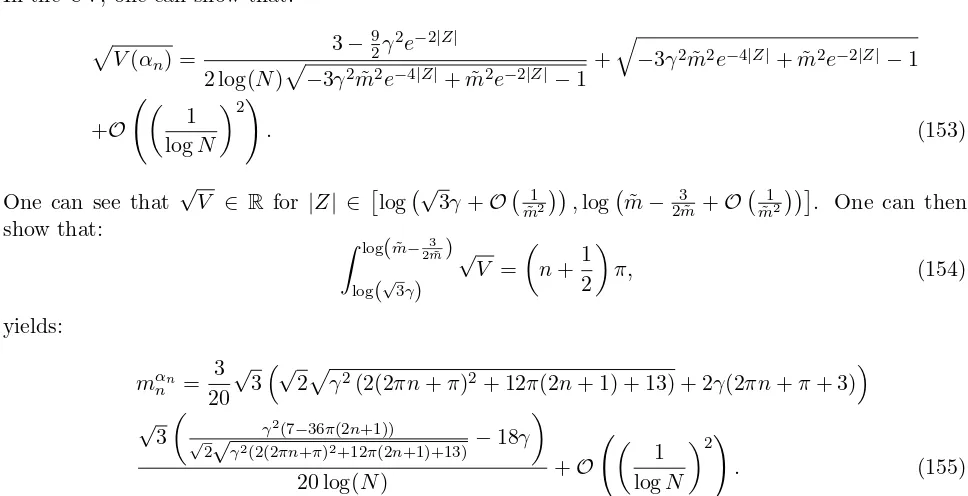
Finally, the WKB quantization condition: Z log(m˜−0m.˜54)

(b) Small-m˜ Expansion We expand

q

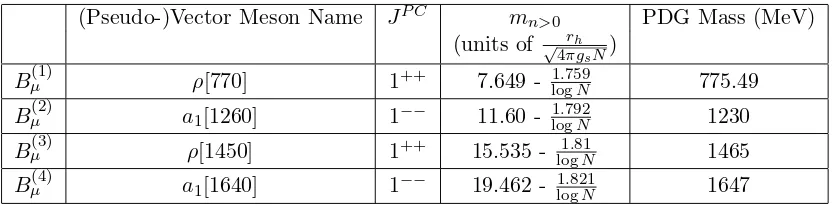
(Pseudo-)Vector Meson Name JP C mn>0 PDG Mass (MeV)

(units of _√ rh

4πgsN)

Bµ(1) ρ[770] 1++ 7.649 - 1_log.759_N 775.49

Bµ(2) a1[1260] 1−− 11.60 - 1_log.792_N 1230

Bµ(3) ρ[1450] 1++ 15.535 - _log1.81_N 1465

Bµ(4) a1[1640] 1−− 19.462 - 1_log.821_N 1647

Table 1: (Pseudo-)Vector Meson masses from WKB Quantization applied to V(α{ni})

the following IR vector meson spectrum is generated:

mn(IR) = 0.5 v u u

t3.036−0.1136logN

0.068logN+ 56.946+ 2.

s

(0.854513n−0.0765252) log2(N) + (715.605n−67.1225)logN−134.138

(0.068logN+ 56.946)2 .

(106)

Happily, the ground state is non-zero and for N = 6000, is 0.81 - not that far off from the value 0.694_{− log}0.155_N in (65) obtained by solving theαn{i}(Z) equation of motion near r =rh or Z = 0 - for

N = 6000 the same yields 0.677.

4.5 α{n0} Spectroscopy from WKB Quantization Writingm= ˜m_√ rh

4πgsN s, a=rh

0.6 + 4gsM2

N (1 + logrh)

, one can obtain the Schr¨odinger-like poten-tial for α{n0}(Z) - due to its cumbersome form, we will not be giving the explicit form of its analytical expression.

After retaining terms up LO inN in the potential, the square root of the Schr¨odinger-like potential forα{n0}(Z) after a large-(log)N expansion yields:

q

Vα{0}n (|Z|, N,m˜) = s

˜

m2_e2|Z|

e4|Z|₋₁ −

1.08 ˜m2

e4|Z|_−1. + 0.e−2|Z|−1.+

e−2|Z| _1.5e2|Z|_−0.81 logNqm˜2e2|Z|

e4|Z|_−1.− 1.08 ˜m 2

e4|Z|₋₁ −1.

+_O 1

logN 2!

. (107)

4.5.1 Large-m˜ Expansion

One can show that V(α{n0})∈Rprovided:

0.5 log0.15 ˜m2₋p25.m˜4_{−108 ˜m}2_{+ 100<|Z|<0.5 log0.15 ˜m}2₊p_{25 ˜m}4_{−108 ˜m}2_{+ 100,}

(108) or

|Z_{| ∈}

0.0385 +_O

1 ˜

m2

,log ˜m₋0.54

˜

m2 +O

1 ˜

m3

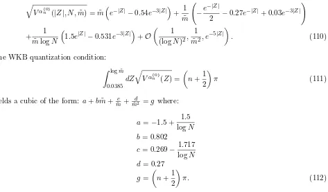
which will be the turning points for the WKB quantization condition implementation. One obtains the following large- ˜m expansion from (107):

q

Vα{0}n ₍|_Z|_{, N,m˜) = ˜m}

e−|Z|−0.54e−3|Z|+ 1 ˜

m − e−|Z|

2 −0.27e

−|Z|_{+ 0.03e}−3|Z| !

+ 1

˜

mlogN

1.5e|Z|−0.531e−3|Z|+O

1 (logN)2,

1 ˜

m2, e− 5|Z|

. (110)

The WKB quantization condition: Z log ˜m

0.0385

dZ q

Vα{0}n (Z) =

n+1 2

π (111)

yields a cubic of the form: a+bm˜ +_m˜c +_m˜d2 =g where:

a=−1.5 + 1.5 logN b= 0.802

c= 0.269− 1.717

logN d= 0.27

g=

n+1 2

π. (112)

The only real root up toO 1 logN

yields the following vector meson spectrum (disregardingn= 0 as it does not satisfy the large- ˜m assumption):

(Pseudo-)Vector Meson Name JP C mn>0 PDG Mass (MeV)

(units of _√ rh

4πgsN)

Bµ(1) ρ[770] 1++ 7.698 - 1_log.604_N 775.49

Bµ(2) a1[1260] 1−− 11.634 - 1_log.692_N 1230

Bµ(3) ρ[1450] 1++ 15.56 - 1_log.736_N 1465

Bµ(4) a1[1640] 1−− 19.483 - 1_log.762_N 1647

Table 2: (Pseudo-)Vector Meson masses from WKB Quantization applied to V(α{n0})

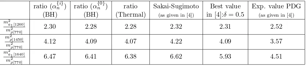
One hence notes a near isospectrality between the (pseudo-)vector meson spectra from Tables 1 and 2, and as will be seen in Table 4, upon comparison with PDG, it is the results of Table 2 that are slightly more closer to the PDG values than those of Table 1.

5

Scalar Meson Spectroscopy using a Black-Hole Background for

All Temperatures

Unlike vector meson spectroscopy, the scalar meson spectrum will be obtained by considering fluctu-ation of the D6-brane world volume alongY by switching off anyD6-brane world-volume fluxes as in [4]. Now, Y ₆= 0 and the D6-brane metric (41), using (49) and the embedding:

Y =Y(xµ, Z), (113)

is therefore:

GIIA_6µνdxµdxν = GIIA_µν 1 +_C1(xκ, Z)Gρλ_IIA∂ρY ∂λY

dxµdxν+_C2(xκ, Z,Y˙)dZ2+C3(xκ, Z,Y˙)dxµdZ∂µY

G_θIIA_2θ2dθ₂2+G_yIIA_˜˜y dy˜2, (114)

where:

C1(xκ, Z) =AY2+BZ2,

C2(xκ, Z,Y˙) = AY2+BZ2

_˙

Y2+ _AY2+_BZ2+ 2Y Z(_{A − B}) ˙Y ,

C3(xκ, Z,Y˙) = 2 AY2+BZ2

_˙

Y + 2Y Z(A − B), (115) wherein:

A= G

IIA

rr r2he2 √

Y2_+Z2

(Y2_+Z2₎ ,

B= G

IIA ˜

z˜z

(Y2_+Z2₎2. (116)

BIIA

N S−N S[2] in diagonal basis (θ2,x,˜ y,˜ z˜) is given by:

BIIA = Bθ2y˜dθ2∧dy˜+Bθ2z˜dθ2∧dz˜+Bθ2x˜dθ2∧dx.˜ (117)

Thus, its pull-back on D6 is given by:

i∗BIIA = Bθ2y˜dθ2∧dy˜+C4(x

κ_{, Z,Y˙)dZ∧dθ}

2+C5(xκ, Z)∂µY dxµ∧dθ2 (118)

where:

C4(xκ, Z,Y˙) =

B_θIIA_2˜z Y2_+Z2

!

˙

Y Z−Y,

C5(xκ, Z) =

B_θIIA_2z˜ Y2_+Z2

!

Z. (119)

Now, Bθ2z˜ and Bθ2˜y are as given in (39).

Therefore:

i∗(G+B)IIA=

A_4×4 B_4×3

C_3×4 D_3×3

where:

(indicated by a tilde below), one obtains:

√

Finally, one thus obtains the following DBI action for Nf D6-branes (setting the tension to unity):

SD6

Now, similar to [4], we make the KK ansatz:

Y(xµ, Z) =X n=1

Y(n)(xµ)_Zn(Z), (123)

Making a field redefinition: Zn(Z) =|Z|Gn(Z), one obtains the following EOM forG(Z):

Gn′′(Z) +Gn′(Z)

1

(2gsNflogN−6gsNf(log(rh) +|Z|) + 8π)2

×

( _2(2g

sNflogN−6gsNf(log(rh) +|Z|) + 8π)

4gsNfe4|Z|logN−12gsNfe4|Z|(log(rh) +|Z|)−3gsNfe4|Z|+ 3gsNf+ 16πe4|Z|

e4|Z|₋₁

−3e−2|Z|

4gsM2log(rh)

N +

4gsM2

N + 0.6

2

×

"

−24gs2Nf2logN(log(rh) +|Z|) + 4gs2Nf2log2(N)−12gs2Nf2logN+ 36gs2Nf2(log(rh) +|Z|)2+ 36gs2Nf2(log(rh) +|Z|)

+18gs2Nf2+ 32πgsNflogN−96πgsNf(log(rh) +|Z|)−48πgsNf + 64π2

#!)

+Gn(Z) ˜

m2_α2 θ12

5

√

N₋α2 θ2

e2|Z|₋3.(4.gsM2log(rh)+4.gsM2+0.6N)2 N2

α2 θ12

5

√

N(e4|Z|₋₁₎ = 0.

(125)

Analogous to obtaining the (pesudo-)vector meson spectrum in Section 4, we will now proceed to obtaining the (pseudo-)scalar meson spectrum by three routes. The first will cater exclusively to an IR computation where we solve the _Gn(Z) EOM near the horizon. Imposing Neumann boundary condition at the horizon results in quantization of the (pseudo-)scalar meson masses. The second route will be to convert theGn(Z) EOM into Schr¨odinger-like EOM and to solve the same in the IR and UV separately and obtain (pseudo-)scalar mass quantization by imposing Neumann boundary conditions at the horizon (IR)/asymptotic boundary (UV). It turns out the former yields a result, which up to LO in N, is of the same order as the IR results of route one. The UV computations satisfy Neumann and/or Dirichlet boundary conditions without any mass quantization condition. The third route catering to the IR-UV interpolating region and what gives us our main results that are directly compared with PDG results, is obtaining the (pseudo-)scalar meson masses via WKB quantization condition.

5.1 Scalar Meson Spectrum from Solution to EOM near r =r_h

Analogous to (58) - (62), one can rewrite (125) and solve the same near r=rh, impose Neumann boundary condition at r=rh with the following identifications:

α1 = 0.92 + 0.24

logN, α2 =

0.02α2_θ2m˜2

α2

θ12 5

√

N +

gsM2m˜2(−3.6 log(rh)−3.6)

N −0.02 ˜m

2_,

β2=−

0.54α2_θ2m˜2

α2

θ12 5

√

N +

gsM2m˜2(7.2 log(rh) + 7.2)

N + 0.54 ˜m

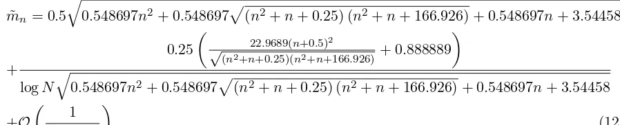
The analog of (62) for scalar mesons up to _Olog1_N: yields:

˜

mn= 0.5

q

0.548697n2_{+ 0.548697}p_(n2_{+n+ 0.25) (n}2_{+n+ 166.926) + 0.548697n+ 3.54458}

+

0.25

22.9689(n+0.5)2

√

(n2_+n+0.25)(n2_+n+166.926)+ 0.888889

logN q

0.548697n2_{+ 0.548697}p_(n2_{+n+ 0.25) (n}2_{+n+ 166.926) + 0.548697n+ 3.54458}

+_O

1 (logN)2

. (127)

The lightest scalar meson masses are:

mn=1 1.331 - 0_log.167_N

mn=2 1.958 - 0_log.226_N

Table 3: The lightest Sector Meson masses

Our result implies that m2n=1

m2

n=0 = 2.16 if one disregards the O

1

N

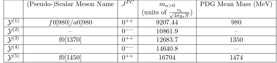
corrections. On comparison with the PDG table for scalar meson masses, if one assumes that the lightest scalar mesons are :

f0[980]/a0[980], f0[1370] then their mass-squared ratio is 1.95 - not too far from our result.

5.2 Scalar Mass Spectrum from Solution of the Schr¨odinger-Like Equation

5.2.1 IR

In the IR, one can show that the potential in a Schr¨odinger-like potential, simplifies to:

V(IR) =

−0.36gs2Nf2log(rh)+2.43gs2Nf2+1.50796gsNf

gs2logN2Nf2 −

0.12

logN −0.02 ˜m2−0.46

|Z|

+13.86gs

4_N

f4log(rh) +gs2Nf2 −2.97gs2Nf2−58.0566gsNf

gs4logN2Nf4

+ 0.54 ˜m2+ 0.25

Z2 −3.413.

(128) The solution to the Schr¨odinger-like equation: Φ′′

n(Z)+V(IR)(Z)Φn(Z) = 0, where Φn(Z) =√C1Gn(Z), and V(IR)(Z) = c1

Z2 +_|a_Z1_|+b1 with:

c1 = 0.25,

, a1 = −

0.36gs2Nf2log(rh) + 2.43gs2Nf2+ 1.50796gsNf

gs2Nf2log2(N) −

0.02 ˜m2− 0.12

log(N)−0.46,

b1 = 0.54 ˜m2−3.413, (129)

is given by:

Φn(Z) =c1Mgs((−0.01 ˜m2 (n)−0.23)logN2₋₀.06logN+1.215)Nf−0.18gslog(_rh)_Nf+0.753982 gslogN2√3.41333−0.54 ˜m2 (n)_Nf ,0

2p3.41333−0.54 ˜m2_(n)|Z|

+c2Wgs((−0.01 ˜m2 (n)−0.23)logN2₋₀.06logN+1.215)Nf−0.18gslog(_rh)_Nf+0.753982 gslogN2√3.41333−0.54 ˜m2 (n)_Nf ,0

Now,

and is hence uninteresting, and will therefore not be implemented. We will implement Neumann boundary condition on Gn(Z) = √Φn(Z)

One can show that: