1
Matrix Algebra
and Solution
of Matrix Equations
1.1 INTRODUCTION
Computers are best suited for repetitive calculations and for organizing data into specialized forms. In this chapter, we review the matrix and vector notation and their manipulations and applications. Vector is a one-dimensional array of numbers and/or characters arranged as a single column. The number of rows is called the order of that vector. Matrix is an extension of vector when a set of numbers and/or characters are arranged in rectangular form. If it has M rows and N column, this matrix then is said to be of order M by N. When M = N, then we say this square matrix is of order N (or M). It is obvious that vector is a special case of matrix when there is only one column. Consequently, a vector is referred to as a column matrix as opposed to the row matrix which has only one row. Braces are conventionally used to indicate a vector such as {V} and brackets are for a matrix such as [M].
rotation about any one of the three axes. It leads to the derivation of the three basic transformation matrices and will be elaborated in detail.
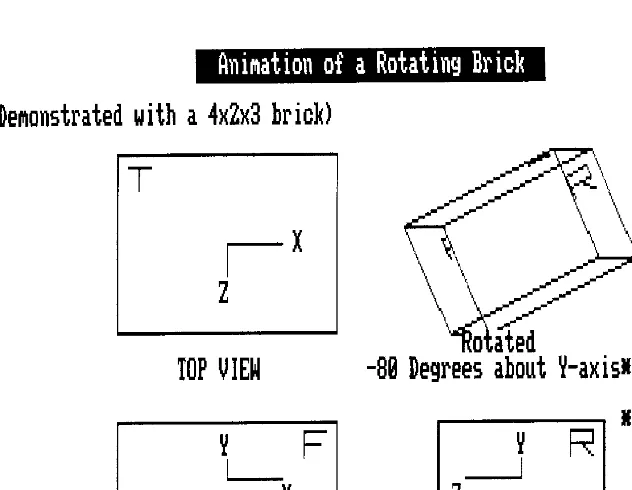
Since the interactive operations of modern personal computers are emphasized in this textbook, how a simple three-dimensional brick can be displayed will be discussed. As an extended application of the display monitor, the transformation of coordinate axes will be applied to demonstrate how animation can be designed to simulate the continuous rotation of the dimensional brick. In fact, any three-dimensional object could be selected and its motion animated on a display screen. Programming languages, FORTRAN, QuickBASIC, MATLAB, and Mathe-matica are to be initiated in this chapter and continuously expanded into higher levels of sophistication in the later chapters to guide the readers into building a collection of their own programs while learning the computational methods for solving engineering problems.
1.2 MANIPULATION OF MATRICES
Two matrices [A] and [B] can be added or subtracted if they are of same order, say M by N which means both having M rows and N columns. If the sum and difference matrices are denoted as [S] and [D], respectively, and they are related to [A] and [B] by the formulas [S] = [A] + [B] and [D] = [A]-[B], and if we denote the elements in [A], [B], [D], and [S] as aij, bij, dij, and sij for i = 1 to M and j = 1 to N, respectively,
then the elements in [S] and [D] are to be calculated with the equations:
(1) and
(2)
Equations 1 and 2 indicate that the element in the ith row and jth column of [S] is the sum of the elements at the same location in [A] and [B], and the one in [D] is to be calculated by subtracting the one in [B] from that in [A] at the same location. To obtain all elements in the sum matrix [S] and the difference matrix [D], the index i runs from 1 to M and the index j runs from 1 to N.
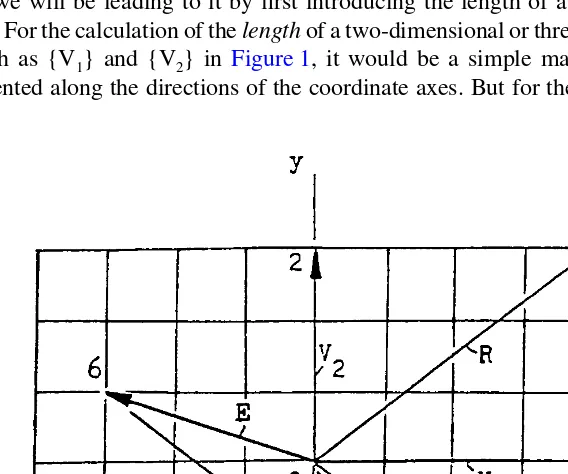
In the case of vector addition and subtraction, only one column is involved (N = 1). As an example of addition and subtraction of two vectors, consider the two vectors in a two-dimensional space as shown in Figure 1, one vector {V1} is directed
from the origin of the x-y coordinate axes, point O, to the point 1 on the x-axis sij=aij+bij
and
When Equation 1 is applied to two arbitrary two-dimensional vectors which unlike {V1}, {V2}, and {V2–} but are not on either one of the coordinate axes, such
as {D} and {E} in Figure 1, we then have the sum vector {F} = {D} + {E} which has components of 1 and –2 units along the x- and y-directions, respectively. Notice that O467 forms a parallelogram in Figure 1 and the two vectors {D} and {E} are the two adjacent sides of the parallelogram at O. To find the sum vector {F} of {D} and {E} graphically, we simply draw a diagonal line from O to the opposite vertex of the parallelogram — this is the well-known Law of Parallelogram.
It should be evident that to write out a vector which has a large number of rows will take up a lot of space. If this vector can be rotated to become from one column to one row, space saving would then be possible. This process is called transposition as we will be leading to it by first introducing the length of a vector.
For the calculation of the length of a two-dimensional or three-dimensional vector, such as {V1} and {V2} in Figure 1, it would be a simple matter because they are
oriented along the directions of the coordinate axes. But for the vectors such as {R}
and {D} shown in Figure 1, the calculation of their lengths would need to know the components of these vectors in the coordinate axes and then apply the Pythagorean theorem. Since the vector {R} has components equal to rx = 4 and ry = 3 units along
the x- and y-axis, respectively, its length, here denoted with the symbol , is:
(3)
To facilitate the calculation of the length of a generalized vector {V} which has N components, denoted as v1 through vN, its length is to be calculated with the
following formula obtained from extending Equation 3 from two-dimensions to N-dimensions:
(4)
For example, a three-dimensional vector has components v1 = vx = 4, v2 = vy =
3, and v3 = vz = 12, then the length of this vector is {V} = [42 + 32 + 122]0.5 = 13.
We shall next show that Equation 4 can also be derived through the introduction of the multiplication rule and transposition of matrices.
1.2 MULTIPLICATION OF MATRICES
A matrix [A] of order L (rows) by M (columns) and a matrix [B] of order M by N can be multiplied in the order of [A][B] to produce a new matrix [P] of order L by N. [A][B] is said as [A] post-multiplied by [B], or, [B] pre-multiplied by [A]. The elements in [P] denoted as pij for i = 1 to N and j = 1 to M are to be calculated
by the formula:
(5)
Equation 5 indicates that the value of the element pij in the ith row and jth column
of the product matrix [P] is to be calculated by multiplying the elements in the ith row of the matrix [A] by the corresponding elements in the jth column of the matrix [B]. It is therefore evident that the number of elements in the ith row of [A] should be equal to the number of elements in the jth column of [B]. In other words, to
More exercises are given in the Problems listed at the end of this chapter for the readers to practice on the matrix multiplications based on Equation 5.
It is of interest to note that the square of the length of a vector {V} which has N components as defined in Equation 4, {V}2, can be obtained by application of
Equation 5 to {V} and its transpose denoted as {V}T which is a row matrix of order
1 by N (one row and N columns). That is:
(6)
For a L-by-M matrix having elements eij where the row index i ranges from 1
to L and the column index j ranges from 1 to M, the transpose of this matrix when its elements are designated as trc will have a value equal to ecr where the row index
r ranges from 1 to M and the column index c ranges from 1 to M because this transpose matrix is of order M by L. As a numerical example, here is a pair of a 3 × 2 matrix [G] and its 2 × 3 transpose [H]:
If the elements of [G] and [H] are designated respectively as gij and hij, then
hij = gji. For example, from above, we observe that h12 = g21 = 5, h23 = g32 = –1, and
so on. There will be more examples of applications of Equations 5 and 6 in the ensuing sections and chapters.
(7)
Let us introduce two vectors, {V} and {R}, which contain the unknown x, y, and z, and the right-hand-side constants in the above three equations, respectively. That is:
(8)
Then, making use of the multiplication rule of matrices, Equation 5, the system of linear algebraic equations, 7, now can be written simply as:
(9)
where the coefficient matrix [C] formed by listing the coefficients of x, y, and z in first equation in the first row and second equation in the second row and so on. That is,
There will be more applications of matrix multiplication and transposition in the ensuing chapters when we discuss how matrix equations, such as [C]{V} = {R}, can be solved by employing the Gaussian Elimination method, and how ordinary differential equations are approximated by finite differences will lead to the matrix equations. In the abbreviated matrix form, derivation and explanation of computa-tional methods becomes much simpler.
Also, it can be observed from the expressions in Equation 8 how the transposition can be conveniently used to define the two vectors not using the column matrices which take more lines.
The resulting display on the screen is:
To review FORTRAN briefly, we notice that matrices should be declared as variables with two subscripts in a DIMENSION statement. The displayed results of matrices A and B show that the values listed between // in a DATA statment will be filling into the first column and then second column and so on of a matrix. To instruct the computer to take the values provided but to fill them into a matrix row-by-row, a more explicit DATA needs to be given as:
statement if not replaced by a statement number, in which formats for printing the listed variables are specified, means “unformatted” and takes whatever the computer provides. For example, statement number 15 is a FORMAT statement used by the WRITE statement preceding it. There are 18 variables listed in that WRITE statement but only six F5.1 codes are specified. F5.1 requests five column spaces and one digit after the decimal point to be used to print the value of a listed variable. / in a FORMAT statement causes the print/display to begin at the first column of the next line. 6F5.1 is, however, enclosed by the inner pair of parentheses that allows it to be reused and every time it is reused the next six values will be printed or displayed on next line. The use (*,*) in a WRITE statement has the convenience of viewing the results and then making a hardcopy on a connected printer by pressing the PrtSc (Print Screen) key.
INTERACTIVE OPERATION
The above program shows that Subroutines are independent units all started with a SUBROUTINE statement which includes a name followed by a pair of parentheses enclosing a number of arguments. The Subroutines are called in the main program by specifying which variables or constants should serve as arguments to connect to the subroutines. Some arguments provide input to the subroutine while other argu-ments transmit out the results determined by the subroutine. These are referred to as input arguments and output arguments, respectively. In many instances, an argu-ment may serve a dual role for both input and output purposes. To construct as an independent unit, a subprogram which can be in the form of a SUBROUTINE, or FUNCTION (to be elaborated later) must have RETURN and END statements.
It should also be remarked that program MatxAlgb is arranged to handle any matrix having an order of no higher than 25 by 25. For this restriction and for having the flexibility of handling any matrices of lesser order, the Lmax, Mmax, and Nmax arguments are added in all three subroutines in order not to cause any mismatch of matrix sizes between the main program and the called subroutine when dealing with any L, M, and N values which are interactively entered via keyboard.
we ought not to write 25 separate statements for the 25 elements in this matrix but derive the indicial formulas for i,j = 1 to 5:
and
Then, the matrix [C] can be generated with the DO loops as follows:
The above short program also demonstrates the use of the CONTINUE state-ment for ending the DO loop(s), and the logical IF statements. The true, or, false condition of the expression inside the outer pair of parentheses directs the computer to execute the statement following the parentheses or the next statement immediately below the current IF statement. Reader may want to practice on deriving indicial formulas and then write a short program for calculating the elements of the matrix:
As another example of writing a computer program based on indicial notation, consider the case of calculating ex based on the infinite series:
(11)
With the understanding that 0! = 1, we have expressed the series as a summation involving the index i which ranges from zero to infinity. A FUNCTION ExpoFunc can be developed for calculating ex based on Equation 11 and taking only a finite
number of terms for a partial sum of the series when the contribution of additional term is less than certain percentage of the sum in magnitude, say 0.001%. This FUNCTION may be arranged as:
To further show the advantage of adopting vector and matrix notation, here let us apply FUNCTION ExpoFunc to examine the surface z(x,y) = ex + y above the
rectangular area 0≤x≤2.0 and 0≤y≤1.5. The following program, ExpTest, will enable us to compare the values of ex + y generated by the FUNCTION ExpoFunc and by
the function EXP available in the FORTRAN library (hence called library function).
The resulting printout is:
It is apparent that two approaches produce almost identical results, so the 0.001% accuracy appears quite adequate for the x and y ranges studied. Also, arranging the results in vector and matrix forms make the presentation much easy to comprehend. We have experienced how the summation process for an indicial formula involv-ing a Σ should be programmed. Another operation symbol of importance is Π which is for multiplication of many factors. That is:
(12)
An obvious application of Equation 12 is for the calculation of factorials. For example, 5! = Πi for i ranges from 1 to 5. As an exercise, we display the values of 1! through 50! with the following program involving a subroutine IFACTO which calculates I! for a specified I value:
ai a a a
i N
N
=
∏
= …1
The resulting print out is (listed in three columns for saving space)
Another application of Equation 12 is for calculation of the binomial coefficients for a real number r and an integer k defined as:
(13)
We shall have the occasion of applying Equations 12 and 13 when the finite differences and Lagrangian interpolation are discussed.
Sample Applications
Program MatxAlgb has been tested interactively, the following are the resulting displays of four test cases:
r k
r r r r k
k
r i i
i k
=
−
(
)
(
−)
… − +(
)
= − +=
∏
1 2 1 1
1
QUICKBASIC VERSION
Notice that the order limit of 25 needed in the FORTRAN version is removed in the QuickBASIC version which allows the dim statement to be adjustable. ' is replacing C in FORTRAN to indicate a comment statement in QuickBASIC. READ and WRITE in FORTRAN are replaced by INPUT and PRINT in QuickBASIC, respectively. The DO loop in FORTRAN is replaced by the FOR and NEXT pair in QuickBASIC.
Sample Applications
MATLAB APPLICATIONS
MATLAB developed by the Mathworks, Inc. offers a quick tool for matrix manipulations. To loadMATLAB after it has been set-up and stored in a subdirectory of a hard drive, say C, we first switch to this subdirectory by entering (followed by pressing ENTER)
C:\cd MATLAB
and then switch to its own subdirectory BIN by entering (followed by pressing ENTER) C:\MATLAB>cd BIN
Next, we type MATLAB to obtain a display of: C:\MATLAB>BIB>MATLAB
Matrix [P] Row 1
0.1400E+02 0.2000E+02 Row 2
A = 1 2 3 4
Notice that the elements of [A] should be entered row by row. While the rows are separated by ;, in each row elements are separated by comma. After the print out of the above results, >> sign will again appear. To eliminate the unnecessary line space (between A = and the first row 1 2), the statement format compact can be entered as follows (the phrase “pressing ENTER key” will be omitted from now on):
>> format compact, B = [5,6;7,8] B =
5 6 7 8
Notice that comma is used to separate the statements. To demonstrate matrix sub-traction and addition, we can have:
>> A-B ans =
–4 –4 –4 –4 >> A + B ans =
6 8
10 12
To apply MATLAB for transposition and multiplication of matrices, we can have: >> C = [1,2,3;4,5,6]
>> D = [1,2,3;4,5,6]; E = [1,2;2,3;3,4]; P = D*E P =
14 20 32 47
Notice that MATLAB uses ' (single quote) in place of the superscripted symbol T for transposition. When ; (semi-colon) follows a statement such as the D statement, the results will not be displayed. As in FORTRAN and QuickBASIC, * is the multiplication operator as is used in P = D*E, here involving three matrices not three single variables. More examples of MATLAB applications including plotting will ensue. To terminate the MATLAB operation, simply enter quit and then the RETURN key.
MATHEMATICA APPLICATIONS
To commence the service of Mathematica from Windows setup, simply point the mouse to it and double click the left button. The Input display bar will appear on screen, applications of Mathematica can start by entering commands from keyboard and then press the Shift and Enter keys. To terminate the Mathematica application, enter Quit[] from keyboard and then press the Shift and Enter keys.
Mathematica commands, statements, and functions are gradually introduced and applied in increasing degree of difficulty. Its graphic capabilities are also utilized in presentation of the computed results.
For matrix operations, Mathematica can compute the sum and difference of two matrices of same order in symbolic forms, such as in the following cases of involving two matrices, A and B, both of order 2 by 2:
In[1]:= A = {{1,2},{3,4}}; MatrixForm[A] Out[1]//MatrixForm =
1 2 3 4
In[3]:= MatrixForm[A + B] Out[3]//MatrixForm=
6 8
10 12
In[4]:= Dif = A-B; MatrixForm[Dif] Out[4]//MatrixForm=
–4 –4 –4 –4
In[3] and In[4] illustrate how matrices are to be added and subtracted, respec-tively. Notice that one can either use A + B directly, or, create a variable Dif to handle the sum and difference matrices.
Also, Mathematica has a function called Transpose for transposition of a matrix. Let us reuse the matrix A to demonstrate its application:
In[5]:= AT = Transpose[A]; MatrixForm[AT] Out[5]//MatrixForm=
1 3 2 4
1.3 SOLUTION OF MATRIX EQUATION
Matrix notation offers the convenience of organizing mathematical expression in an orderly manner and in a form which can be directly followed in coding it into programming languages, particularly in the case of repetitive computation involving the looping process. The most notable situation is in the case of solving a system of linear algebraic equation. For example, if we need to determine a linear equation y = a1 + a2x which geometrically represents a straight line and it is required to pass
through two specified points (x1,y1) and (x2,y2). To find the values of the coefficients
To facilitate programming, it is advantageous to write the above equations in matrix form as:
(3)
where:
(4)
The matrix equation 3 in this case is of small order, that is an order of 2. For small systems, Cramer’s Rule can be conveniently applied which allows the unknown vector {A} to be obtained by the formula:
(5)
Equation 5 involves the calculation of three determinants, i.e., , [C1], [C2], and
[C] where [C1] and [C2] are matrices derived from the matrix [C] when the first
and second columns of [C] are replaced by {Y}, respectively. If we denote the elements of a general matrix [C] of order 2 by cij for i,j = 1,2, the determinant of
[C] by definition is:
(6)
The general definition of the determinant of a matrix [M] of order N and whose elements are denoted as mij for i,j = 1,2,…,N is to add all possible product of N
elements selected one from each row but from different column. There are N! such products and each product carries a positive or negative sign depending on whether even or odd number of exchanges are necessary for rearranging the N subscripts in increasing order. For example, in Equation 6, c11 is selected from the first row and
first column of [C] and only c22 can be selected and multiplied by it while the other
possible product is to select c12 from the second row and first column of [C] and
that leaves only c21 from the second row and first column of [C] available as a factor
of the second product. In order to arrange the two subscripts in non-decreasing order, one exchange is needed and hence the product c c carries a minus sign. We shall
and
Consequently, according to Equation 5 we can find the coefficients in the straight-line equation to be:
Hence, the line passing through the points (1,2) and (3,4) is y = a1 + a2x = 1 + x.
Application of Cramer’s Rule can be extended for solving three unknowns from three linear algebraic equations. Consider the case of finding a plane which passes three points (xi,yi) for i = 1 to 3. The equation of that plane can first be written as
z = a1 + a2x + a3y. Similar to the derivation of Equation 3, here we substitute the
three given points into the z equation and obtain:
(7)
(8)
and
(9)
Again, the above three equations can be written in matrix form as:
And, the Cramer’s Rule for solving Equation 10 can be expressed as:
(12)
where [Ci] for i = 1 to 3 for matrices formed by replacing the ith column of the
matrix [C] by the vector {Z}, respectively. Now, we need the calculation of the determinant of matrices of order 3. If we denote the element in a matrix [M] as mij
for i,j = 1 to 3, the determinant of [M] can be calculated as:
(13)
Rule and the definition of determinant of a 3 by 3 square matrix according to Equations 12 and 13, respectively. First, a subroutine called Determ3 is created explicitly following Equation 13 as listed below:
1.4 PROGRAM GAUSS
Program Gauss is designed for solving N unknowns from N simultaneous, linear algebraic equations by the Gaussian Elimination method. In matrix notation, the problem can be described as to solve a vector {X} from the matrix equation:
(1)
where [C] is an NxN coefficient matrix and {V} is a Nx1 constant vector, and both are prescribed. For example, let us consider the following system:
(2)
(3)
(4)
If the above three equations are expressed in matrix form as Equation 1, then:
(5,6)
and
(7)
where T designates the transpose of a matrix. GAUSSIAN ELIMINATION METHOD
A systematic procedure named after Gauss can be employed for solving x1, x2,
and x3 from the above equations. It consists of first dividing Equation 28 by the
leading coefficient, 9, to obtain:
(9) and
(10)
If we subtract Equation 9 from Equation 3, and subtract Equation 10 from Equa-tion 4, the x1 terms are eliminated. The resulting equations are, respectively:
(11) and
(12)
This completes the first elimination step. The next normalization is applied to Equation 11, and then the x2 term is to be eliminated from Equation 12. The resulting
equations are:
(13) and
(14)
The last normalization of Equation 14 then gives:
(15)
Equations 8, 13, and 15 can be organized in matrix form as:
(16)
The coefficient matrix is now a so-called upper triangular matrix since all
Once, both x2 and x3 have been calculated, x1 can be obtained from Equation 8 as:
To derive a general algorithm for the Gaussian elimination method, let us denote the elements in [C], {X}, and {V} as ci,j, xi, and vi, respectively. Then the
normal-ization of the first equation can be expressed as:
(17)
and
(18)
Equation 17 is to be used for calculating the new coefficient associated with xj
in the first, normalized equation. So, j should be ranged from 2 to N which is the number of unknowns (equal to 3 in the sample case). The subscripts old and new are added to indicate the values before and after normalization, respectively. Such designation is particularly helpful if no separate storage in computer are assigned for [C] for the values of its elements. Notice that (c1,1)new = 1 is not calculated.
Preserving this diagonal element enables the determinant of [C] to be computed. (See the topic on matrix inversion and determinant.)
The formulas for the elimination of x1 terms from the second equation are:
(19)
for j = 2,3,…,N (there is no need to include j = 1) and
(20)
By changing the subscript 2 in Equations 19 and 20, x1 term in the third equation
(22)
Instead of normalizing the first equation, we can generalize Equations 17 and 18 for normalization of the ith equation, for i = 1,2,…,N to the expressions:
(23)
for j = i + 1,i + 2,…,N and
(24)
Note that (ci,i)new should be equal to 1 but no need to calculate since it is not
involved in later calculation for finding {X}.
Similarly, elimination of xi term from kth equation for k = i + 1,i + 2,…,N
consists of using the general formula:
(25)
for j = i + 1,i + 2,…,N and
(26)
Backward substitution for finding xi involves the calculation of:
(27)
for i = N–1,N–2,…,2,1. Note that xN is already found equal to vN after the Nth
normalization.
Program Gauss listed below in both QuickBASIC and FORTRAN languages
QUICKBASIC VERSION
Sample Application
GAUSS-JORDAN METHOD
One slight modification of the elimination step will make the backward substi-tution steps completely unnecessary. That is, during the elimination of the xi terms
from the linear algebraic equations except the ith one, Equations 25 and 26 should be applied for k equal to 1 through N and excluding k = i. For example, the x3 terms
should be eliminated from the first, second, fourth through Nth equations. In this manner, after the Nth normalization, [C] becomes an identity matrix and {V} will have the elements of the required solution {X}. This modified method is called Gauss-Jordan method.
A subroutine called GauJor is made available based on the above argument. In this subroutine, a block of statements are also added to include the consideration of the pivoting technique which is required if ci,i = 0. The normalization steps,
Equations 49 and 50, cannot be implemented if ci,i is equal to zero. For such a
situation, a search for a nonzero ci,k is necessary for i = k + 1,k + 2,…,N. That is,
to find in the kth column of [C] and below the kth row a nonzero element. Once this nonzero ci,k is found, then we can then interchange the ith and kth rows of [C]
and {V} to allow the normalization steps to be implemented; if no nonzero ci,k can
A subroutine has been written based on the Gauss-Jordan method and called GauJor.Sub. Both QuickBASIC and FORTRAN versions are made available and they are listed below.
Sample Applications
The same problem previously solved by the program Gauss has been used again but solved by application of subroutine GauJor. The results obtained with the Quick-BASIC and FORTRAN versions are listed, in that order, below:
MATLAB APPLICATIONS
to solve for {X} when the coefficient matrix [A] and the right-hand side vector {R} are both provided. The following is an example of interactive application:
In[1]:= A = {{3,6,14},{6,14,36},{14,36,98}} Out[1]:=
{{3, 6, 14}, {6, 14, 36}, {14, 36, 98}} In[2]:= MatrixForm[A]
Out[2]//MatrixForm:=
3 6 14
6 14 36 14 36 98 In[3]:= R = {9,20,48} Out[3]:=
{9, 20, 48}
In[4]:= LinearSolve[A,R] Out[4]:=
{–9,13,–3}
Output[2] and Output[1] demonstrate the difference in display of matrix [A] when MatrixeForm is requested, or, not requested, respectively. It shows that without requesting of MatrixForm, some screen space saving can be gained. Output[4] gives the solution {X} = [–9 13 –3]T for the matrix equation [A]{X} = {R} where the
coefficient matix [A] and vector {R} are provided by Input[1] and Input[3], respectively.
1.5 MATRIX INVERSION, DETERMINANT, AND PROGRAM MatxInvD
Given a square matrix [C] of order N, its inverse as [C]–1 of the same order is defined
by the equation:
(1)
C C C C I
To find [C]–1, let c
ij and dij be the elements at the ith row and jth column of the
matrices [C] and [C]–1, respectively. Both i and j range from 1 to N. Furthermore,
let {Dj} and {Ij} be the jth column of the matrices [C]–1 and [I], respectively. It is
easy to observe that {Ij} has elements all equal to zero except the one in the jth row
which is equal to unity. Also,
(3) and
(4)
Based on the rules of matrix multiplication, Equation 1 can be interpreted as [C]{D1} = {I1}, [C]{D2} = {I2}, …, and [C]{DN} = {IN}. This indicates that program
Gauss can be successively employed N times by using the same coefficient matrix [C] and the vectors {Ii} to find the vectors {Di} for i = 1,2,…,N. Program MatxInvD
is developed with this concept by modifying the program Gauss. It is listed below along with a sample interactive run.
QUICKBASIC VERSION
Dj d dlj j dNj T
{ }
=[
2…]
C D D DN
T
[ ]
−1=[
…]
Sample Application
Sample Applications
MATLAB APPLICATION
MATLAB offers very simple matrix operations. For example, matrix inversion can be implemented as:
To check if the obtained inversion indeed satisfies the equation [A}[A]–1 = [I]
where [I] is the identity matrix, we enter:
Once [A]–1 becomes available, we can solve the vector {X} in the matrix equation
[A]{X} = {R} if {R} is prescribed, namely {X} = [A]–1{R}. For example, may enter
MATHEMATICA APPLICATIONS
Mathematica has a function called Inverse for inversion of a matrix. Let us reuse the matrix A that we have entered in earlier examples and continue to dem-onstrate the application of Inverse:
In[1]:= A = {{1,2},{3,4}}; MatrixForm[A] Out[1]//MatrixForm=
1 2 3 4
In[2]:= B = {{5,6},{7,8}}; MatrixForm[B] Out[2]//MatrixForm=
5 6 7 8
In[3]:= MatrixForm[A + B] Out[3]//MatrixForm=
6 8
10 12
In[4]:= Dif = A-B; MatrixForm[Dif] Out[4]//MatrixForm=
–4 –4 –4 –4
In[5]:= AT = Transpose[A]; MatrixForm[AT] Out[5]//MatrixForm=
1 3 2 4
To verify whether or not the inverse matrix Ainv obtained in Output[6] indeed satisfies the equations [A][A]–1 = [I] which is the identity matrix, we apply
Math-ematica for matrix multiplication:
In[7]:= Iden = A.Ainv; MatrixForm[Iden] Out[7]//MatrixForm=
1 0 0 1
A dot is to separate the two matrices A and Ainv which is to be multiplied in that order. Output[7] proves that the computed matrix, Ainv, is the inverse of A! It should be noted that D and I are two reserved variables in Mathematica for the determinant of a matrix and the identity matrix. In their places, here Dif and Iden are adopted, respectively. For further testing, we show that [A][A]T is a symmetric matrix:
In[8]: = S = A.AT; MatrixForm[S] Out[8]//MatrixForm=
5 11 11 25
And, the unknown vector {X} in the matrix equation [A]{X} = {R} can be solved easily if {R} is given and [A]–1 are available:
In[9]:= R = {13,31}; X = Ainv.R Out[9] = {5, 4}
The solution of x1 = 5 and x2 = 4 do satisfy the equations x1 + 2x2 = 13 and 3x1
+ 4x2 = 31.
TRANSFORMATIONOF COORDINATE SYSTEMS, ROTATION, AND ANIMATION
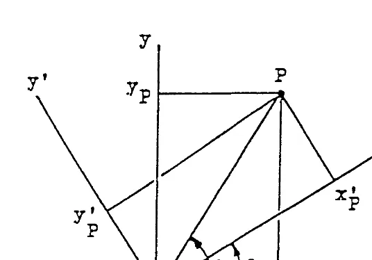
Matrix algebra can be effectively applied for transformation of coordinate sys-tems. When the cartesian coordinate system, x-y-z, is rotated by an angle z about
and
In matrix notation, we may define {P} = [xP yP zP]T and {P'} = [xP' yP' zP']T and
write the above equations as {P'} = [Tz]{P} where the transformation matrix for a
rotation of z-axis by z is:
(5)
In a similar manner, it can be shown that the transformation matrices for rotating about the x- and y-axes by angles x and y, respectively, are:
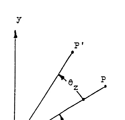
It is interesting to note that if a point P whose coordinates are (xP,yP,zP) is rotated
to the point P' by a rotation of z as shown in Figure 3, the coordinates of P' can
be easily obtained by the formula {P'} = [Rz]{P} where [Rz] = [Tz]T. If the rotation
is by an angle x or y, then {P'} = [Rx]{P} or {P'} = [Ry]{P} where [Rx] = [Tx]T
and [Ry] = [Ty]T.
FUNCTION ANIMATE1(NCYCLE,DAMPING)
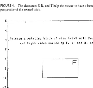
Notice that the coordinates for the corners of the brick are defined in arrays xb, yb, and zb. The coordinates of the points to be connected by linear segments for drawing the characters F, R, ant T are defined in arrays xf, yf, and zf, and xr, yr, and zr, and xt, yt, and zt, respectively.
The equations in deriving [Rx] ( = [Tx]T) and [Ry] ( = [Ty]T) are applied for
x-and y- rotations in the above program. Angle increments of 5 x-and 10° are arranged for the x- and y-rotations, respectively. The rotated views are plotted using the new coordinates of the points, (xbn,ybn,zbn), (xfn,yfn,zfn), etc. Not all of these new arrays but only those needed in subsequent plot are calculated in this m file.
scales in both x- and y-directions. The values in xs and ys arrays also control where to properly place the texts in Figure 4 as indicated in the text statements.
QUICKBASIC VERSION
A QuickBASIC version of the program Animate1.m called Animate1.QB also is provided. It uses commands GET and PUT to animate the rotation of the 4 3 2 brick. More features have been added to show the three principal views of the brick and also the rotated view at the northeast corner of screen, as illustrated in
Figure 6.
The window-viewport transformation of the rotated brick for displaying on the screen is implemented through the functions FNTX and FNTY. The actual ranges of the x and y measurements of the points used for drawing the brick are described by the values of V1 and V2, and V3 and V4, respectively. These ranges are mapped
1.6 PROBLEMS
MATRIX ALGEBRA
4. Apply the QuickBASIC and FORTRAN versions of the program Matx-Algb to verify the results of Problems 1, 2, and 3.
5. Repeat Problem 4 but use MATLAB.
6. Apply the program MatxInvD to find [C]–1 of the matrix [C] given in
Problem 1 and also to ([C]T)–1. Is ([C]–1)T equal to ([C]T)–1?
7. Repeat Problem 6 but use MATLAB.
8. For statistical analysis of a set of N given data X1, X2, …, XN, it is often
necessary to calculate the mean, m, and standard deviation, 5, by use of the formulas:
and
Use indicial notation to express the above two equations and then develop a subroutine meanSD(X,N,RM,SD) for taking the N values of X to compute the real value of mean, RM, and standard deviation, SD. 9. Express the ith term in the following series in indicial notation and then
write an interactive program SinePgrm allowing input of the x value to calculate sin(x) by terminating the series when additional term contributes less than 0.001% of the partial sum of series in magnitude:
Notice that Sin(x) is an odd function so the series contains only terms of odd powers of x and the series carries alternating signs. Compare the result of the program SinePgrm with those obtained by application of the library function Sin available in FORTRAN and QuickBASIC. 10. Same as Problem 9, but for the cosine series:
GAUSS
1. Run the program GAUSS to solve the problem:
2. Run the program GAUSS to solve the problem:
What kind of problem do you encounter? “Divided by zero” is the mes-sage! This happens because the coefficient associated with x1 in the first
equation is equal to zero and the normalization in the program GAUSS cannot be implemented. In this case, the order of the given equations needs to be interchanged. That is to put the second equation on top or find below the first equation an equation which has a coefficient associated with x1 not equal to zero and is to be interchanged with the first equation.
This procedure is called “pivoting.” Subroutine GauJor has such a feature incorporated, apply it for solving the given matrix equation.
3. Modify the program GAUSS by following the Gauss-Jordan elimination procedure and excluding the back-substitution steps. Name this new pro-gram GauJor and test it by solving the matrix equations given in Problems 1 and 2.
6. Apply the Gauss-Jordan elimination method to solve for x1, x2, and x3
from the following equations:
Show every normalization, elimination, and pivoting (if necessary) steps of your calculation.
7. Solve the matrix equation [A]{X} = {C} by Gauss-Jordan method where:
Show every interchange of rows (if you are required to do pivoting before normalization), normalization, and elimination steps by indicating the changes in [A] and {C}.
8. Apply the program GauJor to solve Problem 7.
9. Present every normalization and elimination steps involved in solving the following system of linear algebraic equations by the Gauss-Jordan Elim-ination Method:
5x1 – 2x2 + x3 = 4
–2x1 + 7x2 – 2x3 = 9
x1 – 2x2 + 9x3 = 40
10. Apply the program Gauss to solve Problem 9 described above. 11. Use MATLAB to solve the matrix equation given in Problem 7. 12. Use MATLAB to solve the matrix equation given in Problem 9. 13. Use Mathematica to solve the matrix equation given in Problem 7. 14. Use Mathematica to solve the matrix equation given in Problem 9.
2. Write a program Invert3 which inverts a given 3 × 3 matrix [A] by using the cofactor method. A subroutine COFAC should be developed for cal-culating the cofactor of the element at Ith row and Jth column of [A] in term of the elements of [A] and the user-specified values of I and J. Let the inverse of [A] be designated as [AI] and the determinant of [A] be designated as D. Apply the developed program Invert3 to generate all elements of [AI] by calling the subroutine COFAC and by using D. 3. Write a QuickBASIC or FORTRAN program MatxSorD which will
perform the addition and subtraction of two matrices of same order. 4. Write a QuickBASIC or FORTRAN program MxTransp which will
perform the transposition of a given matrix.
5. Translate the FORTRAN subroutine MatxMtpy into a MATLAB m file so that by entering the matrices [A] and [B] of order L by M and M by N, respectively, it will produce a product matrix [P] of order L by N. 6. Enter MATLAB commands interactively first a square matrix [A] and
then calculate its trace.
7. Use MATLAB commands to first define the elements in its upper right corner including the diagonal, and then use the symmetric properties to define those in the lower left corner.
8. Convert either QuickBasic or FORTRAN version of the program Matx-InvD into a MATLAB function file MatxMatx-InvD.m with a leading statement function [Cinv,D] = MatxInvD(C,N)
9. Apply the program MatxInvD to invert the matrix:
Verify the answer by using Equation 1. 10. Repeat Problem 9 but by MATLAB operation. 11. Apply the program MatxInvD to invert the matrix:
15. What will be the coordinates for the point P mentioned in Problem 14 if the coordinate axes are rotated counterclockwise about the z-axis by 45°?
Use MATLAB to find your answer.
16. Apply MATLAB to find the location of a point whose coordinates are (1,2,3) after three rotations in succession: (1) about y-axis by 30°, (2) about z-axis by 45° and then (3) about x-axis by –60°.
17. Change m file Animate1.m to animate just the rotation of the front (F) side of the 4 2 3 brick in the graphic window.
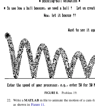
18. Write a MATLAB m file for animation of pendulum swing1 as shown in
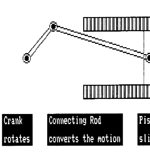
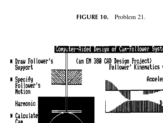
22. Write a MATLAB m file to animate the motion of a cam-follower system as shown in Figure 11.
23. Write a MATLAB m file to animate the rotary motion of a wankel cam as shown in Figure 12.
24. Repeat Problem 9 but by Mathematica operation. 25. Repeat Problem 11 but by Mathematica operation. 26. Repeat Problem 14 but by Mathematica operation. 27. Repeat Problem 15 but by Mathematica operation. 28. Repeat Problem 16 but by Mathematica operation.
1.7 REFERENCE
1. Y. C. Pao, “On Development of Engineering Animation Software,” in Computers in Engineering, edited by K. Ishii, ASME Publications, New York, 1994, pp. 851–855.