THE IMPACT OF SPATIAL AND TEMPORAL RESOLUTIONS IN TROPICAL SUMMER
RAINFALL DISTRIBUTION: PRELIMINARY RESULTS
Qian Liu1,2, Long S Chiu2,* , Xianjun Hao1
1Department of Geography and GeoInformation Science, George Mason University, Fairfax, VA 22030 2Department of Atmospheric, Oceanic, and Earth Sciences George Mason University, Fairfax, VA 22030
(qliu6, lchiu,xhao1)@gmu.edu
KEY WORDS: TRMM data, Rainfall amount, KS test, Temporal resolution, Spatial resolution
ABSTRACT:
The abundance or lack of rainfall affects peoples’ life and activities. As a major component of the global hydrological cycle (Chokngamwong & Chiu, 2007), accurate representations at various spatial and temporal scales are crucial for a lot of decision making processes. Climate models show a warmer and wetter climate due to increases of Greenhouse Gases (GHG). However, the models’ resolutions are often too coarse to be directly applicable to local scales that are useful for mitigation purposes. Hence disaggregation (downscaling) procedures are needed to transfer the coarse scale products to higher spatial and temporal resolutions. The aim of this paper is to examine the changes in the statistical parameters of rainfall at various spatial and temporal resolutions. The TRMM Multi-satellite Precipitation Analysis (TMPA) at 0.25 degree, 3 hourly grid rainfall data for a summer is aggregated to 0.5,1.0, 2.0 and 2.5 degree and at 6, 12, 24 hourly, pentad (five days) and monthly resolutions. The probability distributions (PDF) and cumulative distribution functions(CDF) of rain amount at these resolutions are computed and modeled as a mixed distribution. Parameters of the PDFs are compared using the Kolmogrov-Smironov (KS) test, both for the mixed and the marginal distribution. These distributions are shown to be distinct. The marginal distributions are fitted with Lognormal and Gamma distributions and it is found that the Gamma distributions fit much better than the Lognormal.
1. INTRODUCATION
Rainfall is an important climatic factor, which not only has huge influence on agriculture, transportation and many other human activities, but also a key parameter in ecology, meteorology and hydrology. Extreme rainfall events result in large scale floods and flash floods which become major hydrological disasters. The lack of rainfall results in droughts that affect food production and other environmental conditions. Therefore, an investigation on rainfall distribution
is needed for both scientific
research such as climatic change, hydrologic circulation and ecological environment, and operational decision making and other applications, such as agriculture irrigation, prevention and reduction of natural disasters.
The characteristics of remote sensing data are the large spatial coverage and the frequent satellites’ revisit times. Rain gauge measurements provide continuous temporal coverage, but are however limited to the sampling areas of the gauge. The analysis of gauge networks is used for input to hydrologic models, however, they are limited by their spatial coverage (Chokngamwong & Chiu, 2007). With the increasing number of meteorological satellites, advances in sensor technology and techniques for merging satellite and gauge products, rainfall products have been widely applied for research and operations.
Since the first meteorological satellite, TIROS-1 launched, satellite global rainfall maps have been developed. With the launch of the Tropical Rainfall Measuring Mission (TRMM) and the Global Precipitation Measurement Mission (GPM), the
*
Corresponding author
collection provided the impetus and satellite rainfall estimation techniques flourished. Kidd (Kidd, 2001) reviewed techniques for rainfall measurements and introduced rainfall climatology. Adler et al (Adler, Negria, Keehnb, & Hakkarinenc, 1993) proposed an approach to estimate mean monthly rainfall by combining the GOES infrared data and SSM/I microwave measurements. Main operational techniques for rainfall estimation are the CMORPH (CPC MORPHing technique) precipitation of NOAA Climatic Prediction Center; and the NASA Goddard Precipitation Rain Profiling algorithms for TRMM (GPROF) and merged techniques for the Global Precipitation Mission (GPM) from NASA and JAXA.
The spatial and temporal rainfall distribution can be characterized by the sensor and the associated sampling strategy. Different spatial and temporal scales in rainfall monitoring can impact rainfall distributions. As indicated by Hamza Varikoden (Varikoden, Preethi, Samah, & Babu, 2011), knowledge of the spatiotemporal distribution of high intensity rain events would be immensely useful for planners, architect and disaster managers to undertake appropriate risk reduction strategies. In this study, the rainfall distribution at different spatial and temporal scales is investigated with the TRMM 3 hourly rainfall products.
2. DATA AND METHOD
2.1 TRMM 3B42V7 Data
(TMPA) algorithm, developed by the National Aeronautics and Space Administration (NASA) Goddard Space Flight Center
(GSFC), which can be
downloaded from https://giovanni.sci.gsfc.nasa.gov/giovanni/. And the TRMM 3B42 data has a 0.25degree spatial resolution and 3 hourly temporal resolution, covering the latitudinal band about 50S-50N for the period 1997 to present. (Kummerow, Barnes, Kozu, Shiue, & Simpson, 1998).
The TRMM/TMPA 3B42 rainfall estimates are produced in four stages: (1) the microwave precipitation estimates are calibrated and combined, (2) infrared precipitation estimates are created using the calibrated microwave precipitation, (3) the microwave and IR estimates are combined, and (4) rescaling to monthly data is applied. Each precipitation field is best interpreted as the precipitation rate effective at the nominal observation time (Huffman, et al., 2007). The sources of its passive Microwave satellite precipitation estimates include: TRMM Microwave Imager (TMI), Special Sensor Microwave Imager (SSMI), Special Sensor Microwave Imager/Sounder (SSMIS) (3B42V7 only), Advanced Microwave Scanning Radiometer-EOS (AMSR-E), Advanced Microwave Sounding Unit-B (AMSU-B), and Microwave Humidity Sounder (MHS) (Chen, et al., 2013). And the IR data are from National Climatic Data Center (NCDC) and Climate Prediction Center (CPC), which are calibrated by the Microwave data according to the algorithm. It also incorporates the latest version 4 of Global Precipitation Climatology Centre (GPCC) full-gauge analysis from 1998 to 2010 and the GPCC monitoring gauge analysis since 2010 (Moazami, et al., 2013).
TRMM 3B42 data covers the tropical area of 50o~ -50oN and 180o ~ -180oE, with an original spatial pixel size of 0.25o *0.25o, so the total pixel number of an original dataset is 1440*400. The TRMM 3B42 data set used in this study is the latest version (3B42V7) for the period from June 1st to August 31st. In this study, the precipitation rates of raw data- every three hour’s measurements are aggregated to 6,12, 24 hourly, pentad and monthly scales at the original 0.25 degree, 1.0, and 2.5 degrees’ grids and stored in separate HDF format files.
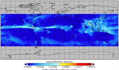
Figure 1. Map of rainfall amount per hour through June 1st to August 31st with a spatial resolution of 0.25o * 0.25o Figure 1 shows the rainfall amount of the study area at a spatial resolution of 0.25 degree. We can observe that higher rainfall
Tropical Convergence Zone (ITCZ). ITCZ is a belt of low pressure which circles the Earth generally near the equator where the trade winds of the Northern and Southern Hemispheres come together. It is characterized by convective activity which generates often vigorous thunderstorms over large areas. Therefore, large amount of rainfall appears there. Other areas of the high rainfall are the maritime continent and the Amazon over land. In addition, there are regions in the western boundaries of the Pacific and Atlantic showing the storm tracks.
2.2 Procedure
Firstly, the separate data files of the same date during the study period are merged into one file in NetCDF format, and a time dimension is created to express time of the data. The monitoring periods of raw data are 00:00~03:00, 03:00~06:00, 06:00~09:00, 09:00~12:00, 12:00~15:00, 15:00~18:00, 18:00~21:00, 21:00~00:00 UTC, corresponding to 8 intervals per day.
The second step is to aggregate these merged data into different temporal and spatial resolutions, and store all the data with the same temporal and spatial resolution into one file in NetCDF format. A time dimension will be created to describe the rainfall amount of one pixel on a given time point. The size of the time dimension is determined by its temporal resolution:
DT = !"#$ ∗ '(
) (1) Where DT is the size of temporal dimension, N+,- is number of days of the study period, and T is the temporal resolution of the satellite rainfall data. Take dataset with a temporal resolution of 3 hour and a spatial resolution of 0.25*0.25 degree as an example, it will have a time dimension size of 92*8(=736). After spatial and temporal aggregation, 3-dimensional datasets of rainfall rate, denoted by Rt,x,y, are obtained for the following statistical analysis. For a set temporal and spatial resolution, its value is equal to the rainfall amount (RAt,x,y) per hour.
And the third step is to analyze the characteristics and difference of and between datasets with different resolutions.
The new rainfall rate on one pixel after temporal aggregation is as follows:
where T is the new temporal resolution; t0 is the time when the monitoring of rainfall rate on the pixel started; x and y is the latitude/longitude coordinates of the pixel, which is not considered to be a variable at this case.
When we fix the temporal resolution, t will not be a variable. Then the rainfall rate of the pixel after aggregated on spatial new spatial resolution; x0, y0 is the original coordinates of the pixel before aggregation.
There are many situations in which the cumulative distribution function contains jumps at some points but is otherwise continuous. Such a distribution is neither discrete nor continuous but rather a combination of a discrete component and a continuous component (Kedem, Chiu, & North, Estimation of Mean Rain Rate: Application to Satellite Observations, 1990). The case of rain rate presents an example of a mixed distribution. For pixels’ RAt,x,y=0, it has a probability 1-p, otherwise the probability is p when RAt,x,y>0. The cumulative distribution function G(r), of RA can be presented as a convex combination of two increasing function H and F, and F is a continuous distribution function (Kedem, Chiu, & North, Estimation of Mean Rain Rate: Application to Satellite Observations, 1990):
G(r) = (1 -p) H(r) + pF(r) (4) generalized density g(r) corresponding to G(r) can be expressed as follow (Aitchison & Brown, 1963):
for
r < 0, g(r) = 0
r=0, g(r)=1-p (5) r> 0, g(r)=pf(r)
Hence the probability of detecting no rain is (1-p) and p is the probability of detecting rain in a space/time element. f(r) is also referred to as the marginal distribution.
2.4 KS test
In statistics, the Kolmogorov–Smirnov test (K–S test or KS test) is a nonparametric test of the equality of continuous, one-dimensional probability distributions that can be used to compare a sample with a reference probability distribution (one-sample K–S test), or to compare two (one-samples (two-(one-sample K–S test). It is named after Andrey Kolmogorov and Nikolai Smirnov (Hazewinkel, 2001).
In this study, KS test is used to test if the distribution of samples from two different resolutions differ. two-sample KS test is used. In this case, the Kolmogorov–Smirnov statistic is
D9,H= sup FM,9(r) − F',H(r) (6) where F1,m(r) and F2,n(r) are the empirical distribution functions of the first and the second sample respectively, and sup is the supremum function. The null hypothesis is that the two sample distributions are different if
D9,H> c 9SH9H (7)
Where c =1.36 at the 95% level and n and m are the number of samples of each dataset. KS tests are performed between distributions of the total distribution (mixed distribution) and the marginal (non-raining) distribution separately.
2.5 Chi-Square Goodness of Fit Test
Parametric tests are also performed using the Lognormal and gamma distribution. This study uses chi-square (X') goodness-of-fit test to compare the distributions, i.e. check how "close" are the observed values to those which would be expected under the fitted model (Department of Statistics and Data Science, n.d.). The X' test estimates the difference between the observed data and the expected value according to the theoretical distribution. If the data are grouped in k categoried (i=1,2,3,…,k), the observed frequency in each class is denoted as O, and the expected probability from the hypothesized distribution is E (CHO, BOWMAN, & NORTH, 2004), then the chi-square test statistic is of the form:
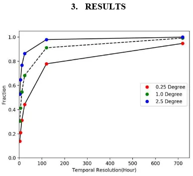
Figure 2. Rain probability in different temporal and spatial resolutions
Figure 2 shows p (rain probability) in different temporal resolutions with spatial resolution of 0.25, 1.0 and 2.5 degrees respectively. It can be found that, with the decrease of temporal and spatial resolutions, the fraction of raining pixels increases and probability of none-rainfall pixels decreases in each spatial resolution, i.e. the larger the observation interval, there is a higher probability of detecting raining events. (Kedem & Chiu, 1987)
3_0.25 12_0.25 daily_0.25 panted_0.25 monthly_0.25
p 0.139 0.311 0.443 0.779 0.948
N 59035625 32998727 23486118 8073365 1637343
Mean(mm/hr) 0.119 0.119 0.119 0.119 0.119
CV 6.286 4.143 3.303 1.975 1.286
Table 1. Rain probability (p), standard deviation (σ), number of samples (N) and mean of datasets in different temporalresolutions with a spatial resolution of 0.25o * 0.25o
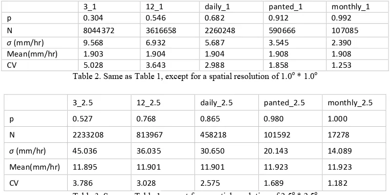
3_1 12_1 daily_1 panted_1 monthly_1
p 0.304 0.546 0.682 0.912 0.992
N 8044372 3616658 2260248 590666 107085
σ (mm/hr) 9.568 6.932 5.687 3.545 2.390
Mean(mm/hr) 1.903 1.904 1.904 1.908 1.908
CV 5.028 3.643 2.988 1.858 1.253
Table 2. Same as Table 1, except for a spatial resolution of 1.0o * 1.0o
3_2.5 12_2.5 daily_2.5 panted_2.5 monthly_2.5
p 0.527 0.768 0.865 0.980 1.000
N 2233208 813967 458218 101592 17278
σ (mm/hr) 45.036 36.035 30.650 20.143 14.089
Mean(mm/hr) 11.895 11.901 11.901 11.923 11.923
CV 3.786 3.028 2.575 1.689 1.182
Table 3. Same as Table 1, except for a spatial resolution of 2.5o * 2.5o Table 1 to Table 3 show the rain probability, standard
deviation(σ), mean value and CV of rainfall rate per hour of different resolutions.
When spatial resolution stays the same and temporal resolution decreases, the mean value doesn’t change because they are derived from the same original data. The slight difference is due to the aggregation process with some missing data. The p value become larger as discussed above. On the other
hand, the variance becomes smaller. That is, the distribution becomes less dispersive. When spatial interval becomes larger, p increases while the mean stay almost the same and the variance decreases if we normalize the data to the same unit area. The coefficient of variations (CV= σ /mean) decrease as the resolution decreases. For example, the CV at the daily temporal resolution are 3.30, 2.99, and 2.58 at spatial resolutions of 0.25, 1.0, and 2.5 degrees.
d D 3_0.25 12_0.25 daily_0.25 panted_0.25 monthly_0.25
3_0.25 0.215 0.278 0.304 0.332
12_0.25 0.0003 0.078 0.126 0.175
daily_0.25 0.0003 0.0004 0.076 0.124
panted_0.25 0.0005 0.0005 0.0006 0.086
monthly_0.25 0.0011 0.0011 0.0011 0.0012
Table 4. KS-test of different temporal resolutions with a spatial resolution of 0.25o * 0.25o
Table 4 shows the D value of KS-test between different temporal resolutions as well as d which refers to the threshold, c*[(n+m)/nm]1/2. Similar tables are constructed at other spatial
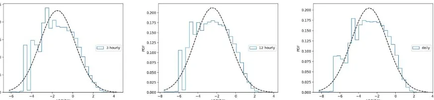
Figure 3. PDF of log value of rainfall rate in different temporal resolutions with a spatial resolution of 0.25o * 0.25o
Figure 4. PDF of log value of value of rainfall in different temporal resolutions with a spatial resolution of 1.0o * 1.0o
Figure 5. PDF of log value of value of rainfall in different temporal resolutions with a spatial resolution of 2.5o * 2.5o
Figure 3 to Figure 5 show the PDF of log rainfall rate at different temporal resolutions with spatial resolutions of 0.25o * 0.25o, 1.0o * 1.0o, and 2.5o * 2.5o. The rainfall amount is binned respectively at 0.42 mm/hr, 1.67 mm/hr and 6.67 mm/hr. It should be noted that the low rain rate data (<0.1mm/hr) deviates substantially from the lognormal distribution. At these low rain rates, the radiometer data used in the algorithm may not be able to discriminate low rain and cloud signatures. The peak of the Lognormal distribution coincides with the data at high resolutions, but shifts toward the low rain rates as the resolutions are degraded. At the mid-high rain rate range, the lognormal distribution underestimates the observed distribution but over-estimates at the high rain end (log r ~ 3). The 12-hourly data fit the lognormal distribution best according to the Chi
square test. For the 3-hourly data, the first half part doesn’t fit the lognormal perfectly as well as the last half part of the daily data.
Another parametric fit to rainfall data in this study is the gamma distribution. Cho et al. (CHO, BOWMAN, & NORTH, 2004) compared the fit of TRMM data to lognormal and gamma distribution and showed that in general the lognormal (gamma) distribution generally fits better in dry (wet) regions. Our data are fitted to these distributions and the fits are compared using the Chi square statistics.
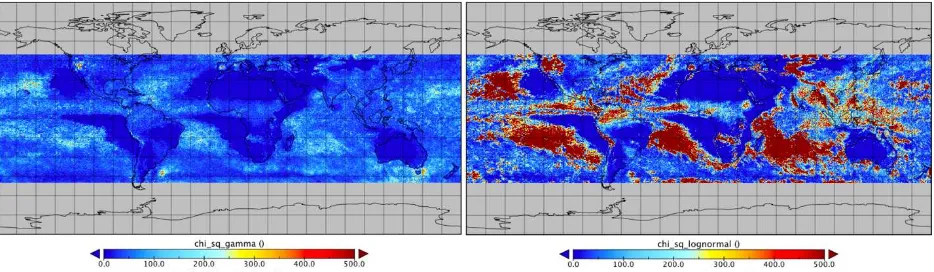
Figure 6. χ2 test of lognormal distribution and gamma distribution in temporal resolution of 3 hourly with a spatial resolution of 0.25o * 0.25o
Figure 7. χ2 test of lognormal distribution and gamma distribution in temporal resolution of 3 hourly with a spatial resolution of 1.0o * 1.0o
Figure 8. χ2 test of gamma distribution and lognormal distribution in temporal resolution of 3 hourly with a spatial resolution of 2.5o * 2.5o
Figure 6 to Figure 8 show the X' value of gamma and lognormal distribution. The observed data of each pixel is generated in 30 groups. In the same temporal and spatial resolution, the
X' value of Gamma distribution is less than that of lognormal
Figure 9. PDF of Lognormal and Gamma distribution fitting to data with temporal resolution of 3 and 12 hourly and spatial resolution of 0.25o * 0.25o
Figure 9 shows PDF of the Lognormal and Gamma distribution. The 3 hourly-0.25degree data is generated in 100 bins and the interval is 0.8mm/hr. Most of the rainfall amount values concentrate in the first few bins. More than 85% is in the first bin which means most of the rainfall amount (per hour) is small than 0.8 mm/hr. The PDF of Gamma distribution fits the observed data well in the first two bins and smaller than the observed PDF in the following bins. The PDF of Lognormal distribution fails to fit the first bin and larger than the observed data in the
following bins. But the first bin of the observed histogram contains most part of the rainfall amount value, therefore the lognormal performs worse than the Gamma distribution. The 12 hourly-0.25degree data is generated in 50 bins and the interval is 1.0mm/hr. The first bin still contains most of the data. The Lognormal distribution fits the first bin better than 3hourly data. It has some improvement in fitting the 12hourly data, but still fail to outperform the Gamma distribution generally.
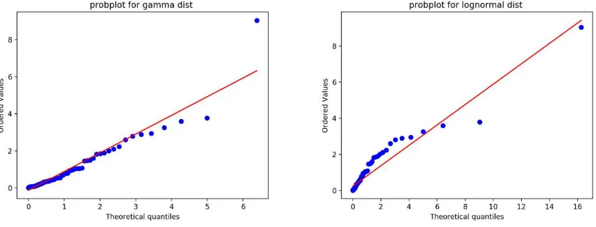
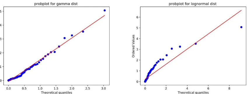
Figure 11. Probplot-plot of Gamma and Lognormal distribution fitting to data with temporal resolution of 12 hourly and spatial resolution of 0.25o * 0.25o
Figure 10 and Figure 11 show Probplot-plot of Gamma and Lognormal distributions fitting to data with temporal resolution of 3 and 12 hourly and spatial resolution of 0.25o * 0.25o. And the paper take 100 samples evenly from each of the original datasets. According to the Probplot-plots, the Gamma distribution fits the datasets better than the Lognormal distribution in both resolutions. And the Gamma fitting result improves when decreasing the temporal resolution, but on the contrary, the Lognormal has a worse fit on the smaller temporal resolution.
4. CONCLUSION
In this study, the characteristics and distribution of rainfall derived from different temporal and spatial resolutions are compared. It is found that: With the decrease of temporal resolution: (1) The fraction of raining pixels (p) becomes larger, as shown in Figure 12. (2) Since the total rainfall amount at any temporal resolution is the same, the conditional rainfall
rate will be decrease according to the relation: CRR= RA/RF, where CRR, RA and RF are the conditional rain rate, rain amount and rain frequency. As temporal resolution decreases, the average conditional rainfall rates become smaller, as shown in Figure 12. (3) As the resolutions decreases, the variance decreases as the data becomes less dispersive (lower CV). (4) The increasing rate of CDF become larger.
And with the decrease of spatial resolution: (1) Raining pixels’ fractions increase and more non-rainfall events are missed, which means an increase on rainfall frequency. This conclusion is also proved by Figure 12. (2) But for pixel area is enlarged with the decrease of spatial resolution, conditional rainfall rate is not comparable between different spatial resolutions. (3) Difference between samples from two spatial resolutions increases when the value of these two resolutions differ greater.
Figure 12. Mean and median of rainfall frequency(RF) and conditional rainfall rate(CRR) in different resolutions.
The study also compare the goodness of fit of the lognormal and gamma distribution. The lognormal fits are in general better over dry areas than over wet areas, consistent with the results of Cho et al. (2004). The gamma distribution performs better than the lognormal distribution both on the
While the datasets are all distinct, there are similarity among some datasets, such as [3hr, 1̊] and [12hr, 0.25̊] when their rain fraction (p) and CV are quite similar. This can be understood in terms of Taylor’s frozen field hypothesis (Gupta & Waymire, 1987), i.e. the field is advected by the mean field, and hence the properties averaged over 3 hourly 1̊ is the same as that at 0.25̊ averaged over 12 hours.
The results herein are only based on one season of data. Our next step is to examine all the available TMPA data and other datasets. Further studies are needed to examine the contributions of the rain fraction and conditional rain rate to the amount at various resolutions, and to examine the scales for which the data are compatible with certain parametric models. The introduction of an autocorrelation scale will also be needed to refine the downscaling model as it has been argued the multi-scale properties of rainfall fields.
REFERENCES
Adler, R. F., Negria, A. J., Keehnb, P. R., & Hakkarinenc, I. M. (1993). Estimation of Monthly Rainfall over Japan and Surrounding Waters from a Combination of Low-Orbit Microwave and Geosynchronous IR Data. Journal of Applied Meteology, 32(2), 335-356.
Aitchison, J., & Brown, J. A. (1963). The Lognormal Distribution (Vol. 3). New York: Cambridge University Press.
Chen, S., Hong, Y., Gourley, J. J., & Huffman, G. J. (2013). Evaluation of the successive V6 and V7 TRMM multisatellite precipitation analysis over the Continental United States. Water Resources Research, 49, 8174–8186.
CHO, H.-K., BOWMAN, K. P., & NORTH, G. R. (2004, November). A Comparison of Gamma and Lognormal Distributions for Characterizing Satellite Rain Rates from the Tropical Rainfall Measuring Mission. 43, 1584-1597.
Chokngamwong, R., & Chiu, L. (2007). Thailand Daily Rainfall and Comparison with TRMM Products. Journal of
Gupta, V. K., & Waymire, E. (1987). On Taylor's hypothesis and dissipation in rainfall. Journal of Geophysical Research: Atmospheres, 92(D8).
Hazewinkel, M. e. (2001). Kolmogorov–Smirnov test. (Springer) Retrieved 6 25, 2017, from Wikipedia: https://en.wikipedia.org/wiki/Kolmogorov%E2%80%93Smirno v_test
Huffman, G. J., Adler, R. F., & Bolvin, D. T. (2007). The TRMM Multisatellite Precipitation Analysis (TMPA): Quasi-Global, Multiyear, Combined-Sensor Precipitation Estimates at Fine Scales. Journal of Hydrometeology, 8, 38-55.
Kedem, B., & Chiu, L. S. (1987). Are rain rate processes self-similar? Water Resource Research, 23(10).
Kedem, B., Chiu, L. S., & North, G. R. (1990, February). Estimation of Mean Rain Rate: Application to Satellite Observations. Journal of Geophysical research, 95, 1965-1972.
Kidd, C. (2001). Satellite rainfall climatology: a review. International Journal of Climatology, 21(9).
Kummerow, C., Barnes, W., Kozu, T., Shiue, J., & Simpson, J. (1998). The tropical rainfall measuring mission (TRMM) sensor package. J. Atmos. Ocean. Technol, 15, 809– 817.
Moazami, S., Golianc, S., Kavianpoura, M. R., & Hongb, Y. (2013). Comparison of PERSIANN and V7 TRMM Multi-satellite Precipitation Analysis (TMPA) products with rain gauge data over IranComparison of PERSIANN and V7 TRMM Multi-satellite Precipitation Analysis (TMPA) products with rain gauge data over Iran. International Journal of Remote Sensing, 34, 8156–8171.