Estimating labor supply of farm households under nonseparability:
empirical evidence from Nepal
Awudu Abdulai
a,∗, Punya Prasad Regmi
baSwiss Federal Institute of Technology, Zurich, Switzerland bAsian Institute of Technology, Bangkok, Thailand
Received 17 June 1999; received in revised form 19 November 1999; accepted 29 December 1999
Abstract
This paper examines the labor supply of farm households in Nepal using a recently developed methodology that accounts for the simultaneity between production and consumption decisions of the households. Estimates of marginal products of male and female labor or shadow wages are obtained from an agricultural production function. An instrumental variable approach is then used to recover the household’s structural labor supply from variations in the shadow wages and income, as well as other household characteristics. The findings reveal that both male and female total labor supply are sensitive to changes in shadow wages and income. Human capital embodied in education is found to exert a significant positive effect on output, but has no statistically significant impact on total labor supply of individuals. The results also rejects the existence of efficient labor markets in rural Nepal. © 2000 Elsevier Science B.V. All rights reserved.
Keywords: Nepal; Agricultural household model; Farm couples; Nonseparability; Local labor markets; Structural estimation; Shadow wage rates
1. Introduction
An understanding of the response of the labor sup-ply of farm households to changes in economic op-portunities is crucial for the achievement of the dual goals of income growth and equity in developing coun-tries. Empirical studies providing information on the determinants of intrafamily allocation of time in pro-ductive activities performed by rural households are particularly important in helping policy makers un-derstand the effects of policies on individual welfare
∗Corresponding author. Tel.:+41-1-632-7930;
fax:+41-1-632-1086.
E-mail address: [email protected] (A. Abdulai)
(Huffman, 1980). In addition, knowledge from such studies may show insight into the intermediary role of the family between public policies and the welfare of family members (Rosenzweig, 1986). More recently, Heckman (1993) argued that empirical evidence on individuals’ labor supply decisions constitutes an im-portant part of the understanding of aggregate labor supply. Considerable effort has therefore been devoted to the analysis of time allocation behavior of rural households in developing countries.
Most of the empirical literature dealing with time allocation of farm households in developing countries are based on the assumption of independence between farm household production and consumption decisions (e.g., Barnum and Squire, 1979; Rosenzweig, 1980;
Ahn et al., 1981). Under this assumption, the farm household acts as if it seeks to maximize profits from its production activities, subject to production con-straints. The resulting farm profits then form part of its full income constraint, subject to which the household is assumed to maximize its utility from consumption. This approach is justifiable algebraically under cer-tain assumptions. The prominent assumptions made are that rural labor markets are efficient and free of transaction costs, and that family and hired labor are perfect substitutes.
While this separability assumption provides analyt-ical advantages for empiranalyt-ical analysis, its shortcom-ings have been clearly documented in the economic literature. Benjamin (1992) points out that market im-perfections that results in hiring-in or off-farm em-ployment constraints, or even differing efficiencies of family and hired labor are all major sources of inter-dependence of production and consumption decisions. Lopez (1984) also argues that farmers may have pref-erences towards working on or off the farm. The sep-arability assumption generally breaks down under any of these conditions. For example, if there are no labor markets, the household must equate its labor demand and supply according to a virtual or shadow wage de-termined by all the variables that influence household decision making (Singh et al., 1986).
Given that rural institutions that pertain to the link-age of factor markets and tenancy rights in developing countries inhibit the working of competitive markets for inputs and output, labor allocation is likely to be determined by shadow wages rather than actual market wages. Recent empirical evidence also call into ques-tion the validity of the perfect substitutability of family and hired labor assumption for developing countries (e.g., Deolalikar and Vijverberg, 1987).
The purpose of this paper is to examine the labor supply responses of males and females of farm house-holds in Nepal to changes in economic opportuni-ties by applying a methodology developed by Jacoby (1993). For policy purposes it is more useful to exam-ine the factors influencing the labor supply responses of males and females separately rather than to note the simple presence of each gender in the household. By following Jacoby’s approach, which permits the analysis of peasant family labor supply behavior under the alternative assumption of nonseparability, the re-strictive assumptions of separability can be eliminated.
Nonseparability between production and consumption decisions implies that a change in any of the exoge-nous variables affecting the production choices of the household — such as changes in the prices of inputs and outputs — will influence the labor supply choices of the household, both directly and indirectly (Singh et al., 1986). While the direct effects occur through changes in the household’s shadow profits, the indirect effects tend to occur through the resulting changes in the shadow wages of family labor.
The paper is laid out as follows. After presenting the theoretical framework in Section 2, Section 3 de-scribes the data used in the study. Empirical results are contained in Section 4 and the paper concludes with a summary section outlining the main findings of this paper.
2. Economic model
The theoretical basis for the model presented be-low draws on the agricultural household model de-veloped in Jacoby (1993) and Skoufias (1994). The model considers a two person household in which both males and females jointly choose the consumption of home produced goods (Q), market goods (G), their re-spective allocation of time (T) between market work (Mi), own-farm work (Fi), home production (Si), and
leisure (Li), as well as the inputs of male and female
hired labor (Hi) into own-farm production, where i
in-dexes males (1) and females (2). Time spent on market work yields wage income that allows the household to purchase the market goods (G). The time allocated to home production involves activities such as child care and meal preparation. The effective real wage earned from off-farm work (Wi) is assumed constant.
It is further assumed that the number of children in the household as well as demographic composition of the adult members of the households are exogenous. Given these specifications the household is assumed to maximize
U=U (C, L1, L2;ZZZ) (1)
category. As in Jacoby (1993), C is total household consumption, which is the sum of home produced (Q) and market purchased goods (G).
The maximization of U is bound by the budget con-straint:
G=Y +W1M1+W2M2−W1hH1−W2hH2+V(2)
where Wi and Wih are the wages of family and
hired labor, respectively, and V is household non-farm nonlabor income net of any fixed costs asso-ciated with farm-household production; the strictly
concave agricultural production function, Y =
Y (F1, F2, H1, H2;EEE), whereEEEis a vector of fixed
in-puts (e.g., land) and Y is farm output. The price of the composite consumption good is normalized to unity and set equal to the price of farm output; the strictly concave home production function, Q=Q(S1, S2;AAA),
whereAAAis a vector of fixed inputs. The agricultural commodity that is either produced by the household or purchased from the market is assumed to be per-fectly substitutable with the home produced commod-ity. The following non-negativity constraints are also assumed to be binding: Si≥0, Mi≥0, Fi≥0, Hi≥0.
In addition, all individuals are assumed to work in at least one sector (Li<Ti).
The first-order conditions for this problem state that each household member equates their marginal rate of substitution between consumption and leisure, or shadow wage, either to their market wage or to their marginal product in either farm work or housework. The decision of some family members not to partici-pate in the labor market results in a budget constraint that is non-linear in hours worked. However, Jacoby (1993) shows that the gradient of the budget constraint is the shadow wage vector (Wˆi) at the optimum, where
ˆ
Wi =YLi, at which point the constraint is linear. This requires redefining the full income of the household as:
male and female time, respectively. Eq. (3) implies that household ‘shadow full income’ (Vˆ) is composed of ‘shadow farm profit’, (5∗) with the opportunity cost of family labor properly deducted and the ‘profit’ from housework (9∗). The household full income constraint evaluated at the optimum is then given as:
G+ ˆQ+ ˆW1L1+ ˆW2L2= ˆV + ˆW1T + ˆW2T (4)
where the expression on the left-hand side is the value of total household expenditures on goods and leisure and the expression on the right-hand side is
the ‘shadow full income’.Qˆ denotes the amount of
the home produced commodity at the optimum Sˆi.
Maximization of Eq. (1) subject to Eq. (4) yields the same first-order conditions as discussed earlier. Solv-ing this revised utility maximization problem yields a set of structural household leisure demand functions:
L∗i =GLi(Wˆ1,Wˆ2,Vˆ;ZZZ), i=1,2 (5)
Given that the shadow wages are the prices of pure leisure in Eq. (5), labor supply can be defined as total hours in productive activities, as opposed to market hours alone as found in traditional labor supply mod-els using observed wages (e.g. Huffman, 1980; Rosen-zweig, 1980). DenotingPi∗as the total hours of work of family males and females in market work, farm pro-duction, and hours used in producing the home good, the structural labor supply functions can be written as:
Pi∗=GPi(Wˆ1,Wˆ2,Vˆ;ZZZ), i=1,2 (6)
wherePi∗=T−L∗i =Si∗+Fi∗+Mi∗, ifMi∗>0, and Pi∗=T−L∗i =Si∗+Fi∗, ifMi∗=0. Male and female labor supply will generally depend on both shadow wages, since men and women are not necessarily per-fect substitutes in production, and separability on the preference side is not imposed.
3. Data and empirical definition of variables
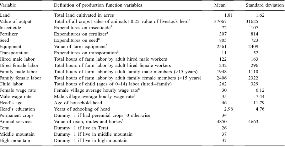
Table 1
Description of the variables used in the estimation of the production function
Variable Definition of production function variables Mean Standard deviation
Land Total land cultivated in acres 1.81 1.62
Value of output Total of all crops+sales of animals+0.25 value of livestock herda 37667 31625
Insecticide Expenditures on insecticidea 72 107
Fertilizer Expenditures on fertilizera 307 814
Seed Expenditures on seeda 805 723
Equipment Value of farm equipmenta 2561 2409
Transportation Expenditures on transportationa 11 52
Hired male labor Total hours of farm labor by adult hired male workers 122 163 Hired female labor Total hours of farm labor by adult hired female workers 242 296 Family male labor Total hours of farm labor by adult family male members (>15 years) 1948 1110 Family female labor Total hours of farm labor by adult family female members (>15 years) 2406 2322 Child labor Total hours of child (ages of 0–14) labor (hired+family) 262 329
Female wage rate Female village average hourly wage ratea 30 6.12
Male wage rate Male village average hourly wage ratea 35 7.44
Head’s age Age of household head 46 11.79
Head’s education Years of schooling of head 2.98 4.76
Permanent crops Dummy: 1 if had perennial crops, 0 otherwise 34
Animal services Value of oxen, mules and horsesa 4850 4663
Terai Dummy: 1 if live in Terai 26
Middle mountain Dummy: 1 if live in middle mountain 37
High mountain Dummy: 1 if live in high mountain 37
a1997 rupees.
period between May 1996 and April 1997. Eight villages were selected to represent the three broad agroclimatic zones of the country. A stratified random sample of a total of 35 households was selected in each of the eight villages to ensure representation of all categories of households. The three zones include the Terai, the Hilly, and the Mountainous zones. The Terai zone which represents the low flat lands of the southern part of the country is very suitable for cereal and vegetable production. The Hilly zone is located in the central part with a climate that ranges between subtropical to temperate. The area is considered very good for fruit production, with cereals and livestock production largely practiced. The Mountainous area, in the northern part of the country, has a climate that is mostly suitable for livestock production and tem-perate fruits, although cereals and potatoes are also cultivated in the area. Mechanization is often difficult on the steep mountain slopes, and households tend to diversify their production activities by cultivating different crops.
The survey collected detailed information on farm and non-farm activities, as well as demographic and
location characteristics. Detailed time allocation in-formation for each household member was collected on a fortnightly basis. Thus, males and females family labor allocated to farm and non-farm activities were fully recorded. Hired labor, differentiated by sex was also included.
Table 1 summarizes the key characteristics of the households. The input of land is measured as amount of land actually used by the household in the year of the survey. Since most households in the sam-ple cultivate more than one crop and also raise live-stock, and data on input use is not available, the ap-proach by Huffman (1976) is followed by aggregat-ing different outputs usaggregat-ing prices. The total value of output is computed as the sum of the value of all crops harvested, the sales of animal products and some fraction of the value of the household’s herd.1 The value of each crop is estimated using village level me-dian prices of the prices that farmers indicate their crops would currently fetch on the market. This avoids
the problem of using the same set of prices for all farms.2
For the variable physical inputs such as fertilizer, insecticides, seeds, and transportation, the only avail-able data are levels of expenditure. Using such data in place of quantities in the production function can lead to biased estimates if input price variation is substan-tial. Including the expenditure levels of these inputs is, however, preferable to ignoring them altogether and suffering an omitted variables problem (Jacoby, 1992). The value of farm equipment (mainly animal ploughs), a dummy variable for whether or not peren-nial crops are grown, and a set of location dummies for Terai, Hilly and Mountainous zones of Nepal are also included as explanatory variables.
Given that better education improves management and may raise technical and allocative efficiency of the individual, education represented by the number of years of schooling is used as an indicator of the poten-tial productivity of the individual. The average head spent about 3 years in school. Female members of the household have a much lower education than males. 38% of males have no education, vs. 64% for females. Age is used as a measure of experience. The use of hired labor is quite low, accounting on average for as little as 7.9% of total labor used in farm production.
4. The empirical estimation
On condition that both household members work on the family farm, estimation of the labor supply functions (6) can be done by substituting the marginal product of family farm labor for the corresponding shadow wage, and by replacing full income with farm profits. As pointed out by Jacoby (1993), if the sam-ple contains part time workers, the market wage could be employed in place of the marginal product of la-bor on the farm, provided working off the farm en-tails no transaction cost. The estimation in the present study proceeds in two steps. Estimates of marginal
2As argued by Bardhan (1979), if farmers face the same prices and the true production possibility frontier is concave, rather than linear, crop composition cannot be allowed to vary across farms, since farmers are assumed to have the same technology. However, if crop composition is variable in the sample, movements along a given production possibility frontier will be construed as shifts in the value of output.
productivity of family male and female labor are first obtained through a production function analysis. The estimated shadow wages and income are then used in the second stage to estimate the male and female labor supply functions.3
4.1. Estimation of the production function
The Cobb–Douglas functional form is used to fit the production function. Despite its well known limi-tations, the Cobb–Douglas form is used because pre-liminary analysis with more flexible functional forms such as the translog, yielded results that were incon-clusive. Specifically, most of the coefficients of the in-teraction terms were not statistically significant, while some of the coefficients turned out to be negative, con-trary to a priori expectations.4 The advantage of the Cobb–Douglas form is its ease of estimation and in-terpretation. The coefficient of an input in the function represents the production elasticity of that input. The production function is specified as:
lnYi =
where Yi represents the total value of agricultural
out-put produced by farm household i, Xij is a vector
de-noting the quantity of input j used by farmer i, DK
is a vector of location dummies that represent some location-specific characteristics, such as topology and temperature, which affect output but are not observ-able to an econometrician;αj andgk are parameters,
and εi is an error term summarizing the effects of
omitted variables. The inputs included in the vector
Xj include cropped area, value of seed, value of
fer-tilizer, value of insecticide, expenditure on
transporta-3 As stated in Lopez (1984), if the production and labor sup-ply disturbance are correlated, then greater efficiency might be achieved by employing a full-information estimation method. Ja-coby (1993), however, points out that even if the production func-tion and the labor supply funcfunc-tions are linear in their parameters, the later functions will generally not be linear in the parame-ters, presenting computational difficulties. The approach of Jacoby (1993) and McCurdy and Pencavel (1986) is therefore followed in this study.
tion, hours of hired male labor, hours of hired female labor, hours of family male labor, hours of family fe-male labor, hours of child labor (family and hired), hours of draft animals services and livestock inputs (mainly medicine and feed).
The age and level of education of household head are also included as proxies for the management input. This is done under the assumption that the household head, whether male or female, is also the primary de-cision maker on the family farm. In the regression, all the independent variables except for the dummies are in logarithmic form. Given the presence of zero values in most of the variable inputs, the logarithmic transfor-mation was carried out by adding one to all the inputs, except land and adult male and female labor which are always positive by construction of the sample.
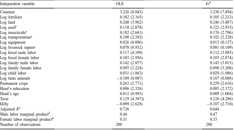
Table 2 reports OLS estimates of the coefficients of the production function. The results indicate that most of the inputs have significantly positive effects on agri-cultural output. Land appears to be an important input in the production process. With the notable exception of child labor, all the variables representing labor are significantly different from zero. The coefficients for the labor variables show that the use of family labor has a greater impact on agricultural output than the use of hired labor, supporting the hypothesis that fam-ily members have stronger work incentives compared to hired labor. Quite striking is the fact that family male labor has a greater impact on output than family female labor. This result is in contrast to the findings reported by Skoufias (1994) who finds that family fe-male labor has a greater impact on output than fam-ily male labor in India. The result here is probably due to the fact that the activities such as ploughing, which are undertaken by men, contribute more at the margin to output than activities such as weeding and transplanting in which females are largely engaged in Nepal. The head’s schooling also has a positive and significant impact on agricultural output, confirming the widely accepted role of human capital toward im-proving farmers’ efficiency (Abdulai and Huffman, 1999). The choice of livestock appreciation rate does not seem to influence the estimated marginal products of male and female labor.5
5When the rate is set at 0.2 or 0.3, instead of 0.25, the resulting marginal products are perfectly correlated with those derived from the estimates reported in Table 2.
Given that the physical inputs themselves are likely to be endogenous variables, the estimates from OLS could be biased. Hence, instrumental vari-able technique (IV) is also applied to estimate the Cobb–Douglas production function. The second col-umn in Table 2 presents the instrumental variable estimates. The variables used as identifying instru-ments in the estimation are indicated at the bottom of Table 2. The value of the Wu–Hausman statistic given in Table 2 suggests that the instruments can be considered exogenous in the estimation. Following Jacoby (1993), the shadow wage rates (or marginal products) of family male and female labor hours are calculated from the instrumental variable estimates of the Cobb–Douglas production presented in Table 2, using the formula:6
whereYˆ is the predicted value of output derived from the estimated coefficientαˆj. F1 and F2 are the total
hours of labor by adult male and female, respectively. The estimates of the shadow income of the household,
ˆ
where 9 is the sum of net returns from sales of
livestock products and trade and handicrafts, V is non-labor income such as land rent and transfers re-ceived by households, W1, W2, Waare village average
wage rates for males, females, and animal services, respectively; FERTV, INSV, and SEEDV are expendi-tures on fertilizer, insecticide, and seeds, respectively.
4.2. Specification of the labor supply functions
The labor supply of males and females are fitted separately to data for the farm households used in the previous analysis. Analysis is focused on impacts of wages, income and other exogenous variables on the
Table 2
Cobb–Douglas production function estimates (dependent variable: log value of output)a
Independent variable OLS Ivb
Constant 3.226 (8.043) 3.230 (7.894)
Log fertilizer 0.102 (2.165) 0.105 (2.213)
Log land 0.248 (3.962) 0.246 (3.887)
Log seedc 0.118 (2.878) 0.122 (2.933)
Log insecticidec 0.182 (2.661) 0.176 (2.706)
Log transportationc 0.108 (2.392) 0.102 (2.228)
Log equipment 0.026 (0.086) 0.013 (0.137)
Log livestock inputsc 0.078 (0.932) 0.081 (0.109)
Log hired male labor 0.117 (4.109) 0.112 (3.885)
Log hired female labor 0.103 (2.956) 0.105 (2.874)
Log family male labor 0.142 (2.857) 0.145 (3.013)
Log family female labor 0.095 (3.224) 0.098 (3.208)
Log child labor 0.031 (1.063) 0.029 (1.086)
Log farm animals −0.109 (0.087) 0.107 (0.088)
Permanent crops 0.263 (2.771) 0.259 (2.616)
Head’s education 0.086 (2.326) 0.085 (2.372)
Head’s age 0.012 (0.983) 0.009 (1.004)
Terai 0.129 (4.307)) 0.126 (4.286)
Hilly −0.099 (2.628) −0.107 (2.710)
Adjusted R2 0.726 0.644
Male labor marginal productd 0.44 0.47
Female labor marginal productd 0.31 0.33
Number of observations 280 280
aAbsolute values of t-statistics in parentheses.
bWu–Hausman statistic for the joint exogeneity test is 15.8 against a critical value ofχ2
(9,0.01)=16.9.
cVariables considered endogenous in the instrumental variable estimation.
dMeans over the sample of 280 households are reported. Computed as given in Eq. (8). The set of instruments used in the production function analysis include male daily field wage, female daily field wage, fraction of land owned, village size dummy (1 if 1500 inhabitants, 0 otherwise), light source dummy (1 if electricity, 0 otherwise), water source dummy (0 from river, 1 otherwise), cooking fuel dummy (0 if use wood, 1 otherwise), village level price if rice, and adults above 60 years old.
total hours worked by males and females. Since all households reported positive hours for male and fe-male farm labor, the entire sample is used. For each household, the male and female labor supply variables are computed as the average number of hours per day spent in farm work, off-farm self-employment, wage employment and housework by males and females in the household, respectively. Time spent on social cer-emonies, religious activities, and other pure consump-tion activities, such as eating or sleeping are consid-ered as leisure. All females in the sample reported positive hours for farm work and domestic activities, while all males reported positive hours for farm work, with some reporting positive hours for domestic ac-tivities. The average daily hours in non-leisure activ-ities (total hours worked) are 8.5 for males and 10.0
for females, indicating that women spend more time in working than men.
The empirical specification of Eq. (5) for males and females are:
lnP1∗=α10+α11lnWˆ1+α12lnWˆ2
+α13lnVˆ +α14Z1+µ1 (10a)
lnP2∗=α20+α21lnWˆ1+α22lnWˆ2
+α23lnVˆ +α24Z2+µ2 (10b)
where Wˆ1, Wˆ2 and Vˆ are as described in the
pre-vious section, Zi is a vector of individual- and/or
compo-sition variables, etc. affecting taste towards work,α’s are parameters to be estimated, andµi is an error term
summarizing the effects of unobserved factors.7 As
in the production function analysis, age and educa-tion are measured in years. Including age in quadratic form allows estimation of life cycle effects. Number of adult males and females, as well as children in the household are also included. The rationale for including children is that women with children of pre-school or primary school age are less likely to have time to engage in market activities.
The coefficients α13 and α23 provide estimates of
the income elasticities of male and female labor, re-spectively. If leisure is a normal good, higher levels of income would result in fewer hours of work. Previ-ous studies generally support this hypothesis although estimates have been inelastic (Jacoby, 1993; Skoufias, 1994). The estimated coefficients α11 and α22
rep-resent the uncompensated own-wage elasticities for males and females, respectively, while α12 and α21
provide estimates of the uncompensated cross-wage elasticities.
To obtain consistent estimates, the labor supply functions are estimated using instrumental variable procedure. In the first-stage, the shadow wage rates and shadow income are regressed on variables of household composition such as the number of chil-dren less than or equal to 14 years, and the number of males and females greater than or equal to 15 years and less than 60 years, individual characteristics such as age and age squared, and number of years of schooling; zonal dummies, value of buildings, land and farm implements owned by the household, and all the instruments that are given in Table 2. The predicted values from these regressions are then used in the second stage to estimate the labor supply functions employing ordinary least squares.
Estimating the labor supply functions with the pre-dicted values requires deleting some variables that are used in the first stage regression to allow for identifica-tion of the models. Household assets such as land and value of buildings, village level wage rates, and the interaction variables were deleted from the labor
sup-7It is significant to mention that the estimated shadow income and marginal products of family male and female labor are house-hold specific and as such take on the same value for different members of the household of the same gender.
ply functions, thus serving as identifying instruments. The Wald test statistics (χ102) for the joint significance of these variables in the shadow wage equations are 20.06 and 24.28 for males and females, respectively, against the critical value of χ(210,0.05) = 18.31. The corresponding figure for the shadow income equation is 23.19, also against a critical value ofχ(210,0.05) =
18.31. The joint significance of these variables in the first stage regressions suggests that the instruments do enter the first stage estimation and are therefore ap-propriate instruments (Staiger and Stock, 1997).
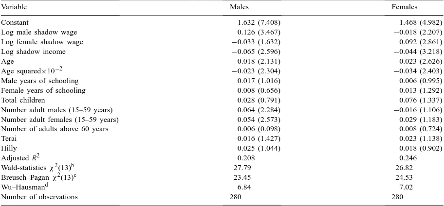
Table 3 presents the parameter estimates of the male and female labor supply functions. The Breusch–Pagan test was employed to test for po-tential heteroskedasticity that may be induced by the two-stage procedure of using estimated shadow wages and income as well as heteroskedasticity pos-sibly present across households. The computed χ132 values of 23.45 and 24.53 for males and females, re-spectively, are above the critical value of 22.4 at the 5% level, suggesting the presence of heteroskedas-ticity. In order to account for the heteroskedasticity, the t-statistics reported are calculated from White’s (White, 1980) formula that accounts for nonpara-metric forms of heteroskedasticity. The values of the Wu–Hausman statistics given in the Table suggest that the instruments can be considered exogenous in the labor supply functions. The joint hypotheses that all non-intercept coefficients in the labor supply models are zero are tested with Wald statistics. The sample values of the Wald statistics8 are 27.79 and 26.82 for the male and female labor supply functions, respectively, with a critical value ofχ132,0.05 =22.4, thus rejecting the null hypotheses.
Consistent with Jacoby’s findings, the estimates of uncompensated own-wage effects are significant and positive for both males and females, suggesting an upward sloping labor supply. The findings, however, contrast with backward bending market labor supply functions reported by Skoufias (1994) for Indian fe-males and Rosenzweig (1980) for Indian fe-males. More-over, the own-wage elasticities are slightly higher for men than for women. Given that the definition of
Table 3
Instrumental variable estimates of male and female labor supply functions using shadow wages and incomea
Variable Males Females
Constant 1.632 (7.408) 1.468 (4.982)
Log male shadow wage 0.126 (3.467) −0.018 (2.207)
Log female shadow wage −0.033 (1.632) 0.092 (2.861)
Log shadow income −0.065 (2.596) −0.044 (3.218)
Age 0.018 (2.131) 0.023 (2.626)
Age squared×10−2 −0.023 (2.304) −0.034 (2.403)
Male years of schooling 0.017 (1.016) 0.006 (0.995)
Female years of schooling 0.008 (0.656) 0.013 (1.292)
Total children 0.028 (0.791) 0.076 (1.337)
Number adult males (15–59 years) 0.064 (2.284) −0.016 (1.106)
Number adult females (15–59 years) 0.054 (2.573) 0.029 (1.183)
Number of adults above 60 years 0.006 (0.098) 0.008 (0.724)
Terai 0.016 (1.427) 0.023 (1.138)
Hilly 0.025 (1.044) 0.018 (0.902)
Adjusted R2 0.208 0.246
Wald-statisticsχ2(13)b 27.79 26.82
Breusch–Paganχ2(13)c 23.45 24.53
Wu–Hausmand 6.84 7.02
Number of observations 280 280
aAbsolute values of White’s t-statistics in parentheses.
bWald test for the joint significance of the non-intercept exogenous variables against a critical value ofχ2
(13,0.05)=22.4.
cBreusch–Pagan test for homoskedasticity.
dWu–Hausman test for exogeneity of the set of instruments against a critical value ofχ2
(3,0.01)=7.81.
labor supply used in this study includes housework, a greater response by females to changes in their shadow wage should not be expected a priori (Jacoby, 1993). Both point estimates of shadow income are significant and negative for males and females, indicating that both male and female leisure are normal goods. The income elasticities are greater for men than women, a finding that is in line with the results obtained by Skoufias (1994) for India, but contrasts with that of Jacoby (1993) for Peru.
The cross male wage effect on the market labor sup-ply of females is negative and significant, indicating that female labor supply is sensitive to movements in the male wage. This is consistent with family utility maximization and indicates that studies that restrict such cross-wage effects to be zero may result in spec-ification errors.
The age variable represents a combination of expe-rience and life-cycle effects on labor supply. The co-efficients suggest that more experience initially tends to increase the market labor supply of individuals, al-though at a decreasing rate. The labor supply of males
and females begin to decrease after the ages of 39.1 and 35.9, respectively. There is no effect of the num-ber of years of schooling on the labor market decisions of households, indicating that the main impact of ed-ucation on male and female labor supply is indirect through farm profitability and marginal productivity of male and female time in farm production. The num-ber of children appears to have no significant impact on the market labor supply of males and females in Nepal, a result that is consistent with findings based on data from other developing countries (Rosenzweig, 1980; Abdulai and Delgado, 1999). The presence of other men and women in the household of working age tends to increase the market labor supply of men. However, the variable representing the number of men of working age in the household has a negative, al-though statistically insignificant effect in the women’s labor supply equation.
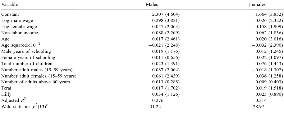
Table 4
Instrumental variable estimates of male and female labor supply functions using market wages and non-labor incomea,b
Variable Males Females
Constant 2.307 (4.604) 1.664 (3.852)
Log male wage −0.298 (3.821) 0.026 (2.322)
Log female wage −0.047 (2.063) −0.158 (1.909)
Non-labor income −0.088 (2.269) −0.062 (1.836)
Age 0.017 (2.461) 0.020 (3.016)
Age squared×10−2 −0.021 (2.248) −0.032 (2.390)
Male years of schooling 0.019 (1.176) 0.012 (1.245)
Female years of schooling 0.011 (0.656) 0.022 (1.097)
Total number of children 0.023 (1.391) 0.076 (1.443)
Number adult males (15–59 years) 0.087 (2.064) −0.018 (1.302)
Number adult females (15–59 years) 0.061 (2.439) 0.036 (1.258)
Number of adults above 60 years 0.013 (0.288) 0.009 (0.403)
Terai 0.017 (1.702) 0.019 (1.518)
Hilly 0.034 (1.126) 0.025 (0.890)
Adjusted R2 0.276 0.314
Wald-statisticsχ2(13)c 31.22 28.97
aAbsolute values of White’s t-statistics in parentheses.
bMale and female market wages are endogenous variables, as such predicted wages are used in estimating the labor supply functions. Wages are predicted with village dummies and land owned as excluded exogenous variables.
cWald test for the joint significance of the non-intercept exogenous variables against a critical value ofχ2
13,0.05=22.4.
(Wi) in place of the shadow wages (Wˆi), and non-labor
income in place of the shadow income (Vˆi). These
results are reported in Table 4. It can be observed that the estimates obtained using market wages differ from those with shadow wages discussed above. In particular, the coefficients for the wage and income variables are much higher, while the own-wage effects are negative for males and females, suggesting that assumptions about separability are crucial in labor supply estimations (Skoufias, 1994).
4.3. Examining the equality of market wage and marginal productivity
In order to gain further insights into the efficient functioning of labor markets in rural Nepal, the hy-pothesis of equality between marginal products of la-bor and the market wages is tested in this section. This is done by using the sub-samples of males and females who report working mostly for wages during the sur-vey period. Approximately 39% of males and 34% of females in the sample fall in this category. Under the assumption that households maximize utility, the ef-fective wage received by family members participat-ing in the non-farm labor market should be equal to
the marginal productivity of work on the family farm. Further assuming that working off the farm entails no transaction cost, the effective wage reported should be equal to the market wage. As in Jacoby (1993), the following regression is estimated to verify the equality of marginal productivity and wage rate
ˆ
Wi =a+bWi+υi, i=1,2 (11)
whereWˆi is the estimated shadow wage of male and
female labor, Wi is the wage received by working in
the market, andυiis a random term probably including
measurement error.
As indicated above, utility maximization and effi-ciency of the labor market imply that a=0, and b=1. This means that the allocation of time between farm and market is made purely on efficiency grounds by individuals in the sub-sample. The theory also implies thatυiis independent of the taste for work. In addition
to the OLS estimates, instrumental variable estimation is also carried out to account for potential measure-ment errors in the wage rates.
Table 5 reports the estimates of Eq. (11). The
F-statistics from the OLS and instrumental variable
Table 5
Tests of the market wages and estimated marginal products for labor market participantsa
ˆ
a bˆ R2 F-testb
Males (n=109)
OLS 0.192 (0.108) 0.737 (0.201) 0.093 23.86 2SLS 0.236 (0.249) 0.814 (0.312) 0.075 19.72 Females (n=95)
OLS 0.414 (0.159) 0.371 (0.126) 0.061 37.63 2SLS 0.863 (0.392) 0.648 (0.230) 0.039 33.78
aStandard errors in parentheses.
bNull hypothesis: (a, b)=(0, 1). The 5% critical value is 3.
product and wage rates can be rejected for both males and females. This finding is in line with the ear-lier results reported by Jacoby (1993) and Skoufias (1994). The presence of transaction costs or other imperfections such as commuting cost or disutility associated with working off the farm, or employment constraints in the labor market, could be responsible for the inequality between the marginal product and the market wage. It is, however, noteworthy that even under these circumstances, the marginal product and the shadow wage would still be equal (Jacoby, 1993). The findings here indirectly lend some support to the concern about interdependence of production and consumption decisions of farm households (Table 5).
5. Concluding remarks
Farm households in developing countries often face partly absent labor markets or institutionally imposed constraints. Under such conditions, households tend to face a shadow wage that depends on both produc-tion technology and household preferences. Hence, it is significant to examine how their labor supply is af-fected by changes in their shadow wages and income. This paper applied a model that permits the estima-tion of the labor supply of farm household members under the assumption of nonseparability between pro-duction and consumption decisions of households to a sample of 280 Nepalese farm households. Estimates of the marginal productivities of family male and fe-male labor were derived from an agricultural produc-tion funcproduc-tion. In a second stage, the estimated shadow wages and income were then used to examine the
response of individual time of work to changes in the economic conditions facing the household.
Evidence was found to support the behavioral assumption that farm households allocate their members’ time as if to maximize a family utility function. The male and female labor supply function estimates appeared similar in many respects to econo-metric labor supply findings based on other devel-oping country data sets. Specifically, the total hours of male and female work were found to be sensitive to changes in the shadow wages and income. An in-crease in the wage rate of a family member tends to have a negative impact on the market labor supply of other family members. These cross wage effects on the labor supply of family members provide evidence on the significant role of the family as an intermediary between public policies and individual welfare.
The results also were consistent with the hypothesis that schooling enhances agricultural productivity in Nepal. In contrast to several studies on labor supply of farm households in developing countries, school-ing did not seem to have a direct effect on either male or female total hours of work. This suggests that the main impact of schooling on male and female mar-ket labor supply is indirect through farm profitability and marginal productivity of male and female time in farm production. Furthermore, the analysis provides evidence against the perfect factor market hypothesis. A finding that is in line with much of the development literature in which inefficient markets are regarded as part of the economic landscape in developing economies.
The methodology employed here provides further information on the usefulness of shadow wages in es-timating time allocation models, particularly where wage data are not available, or the conditions required to make use of available wage data are not in place. This information is essential to establish distributional impacts of changing economic conditions on farm household welfare.
Acknowledgements
dur-ing his stay. He also acknowledges financial support from the German Technical Cooperation and Swiss Agency for Development and Cooperation for the data collection. The first author also benefited from ear-lier discussions with Wallace Huffman. The authors wish to thank two anonymous referees for valuable comments on an earlier version of this paper.
References
Abdulai, A., Huffman, W.E., 1999. Structural Adjustment and Efficiency of Rice Farmers in Northern Ghana. Econ. Dev. Cult. Change, in press.
Abdulai, A., Delgado, C., 1999. Determinants of nonfarm earnings of farm-based husbands and wives in Northern Ghana. Am. J. Agric. Econ. 81, 117–130.
Ahn, C.Y., Singh, I., Squire, L., 1981. The model of an agricultural household in a multi-crop economy: the case of Korea. Rev. Econ. Stat. 63, 520–525.
Bardhan, P.K., 1979. Wages and employment in a poor agrarian economy: a theoretical and empirical analysis. J. Pol. Econ. 87, 479–500.
Barnum, H., Squire, L., 1979. An econometric application of the theory of the farm household. J. Dev. Econ. 60, 79–102. Benjamin, D., 1992. Households composition, labor markets, and
labor demand: testing for separation in agricultural households models. Econometrica. 60, 287–322.
Deolalikar, A.B., Vijverberg, W., 1987. A test of the heterogeneity of family and hired labor in Asian agriculture. Oxf. Bull. Econ. Stat. 49, 291–305.
Greene, W.H., 1997. Econometric Analysis, 3rd Edition. Macmillan, New York.
Heckman, J., 1993. What has been learned about labor supply in the past twenty years? Am. Econ. Rev. 83, 116–121. Huffman, W.E., 1980. Farm and off-farm work decisions: the role
of human capital. Rev. Econ. Stat. LXII, 14–23.
Huffman, W.E., 1976. The productive value of human time in US agriculture. Am. J. Agric. Econ., 672–683.
Jacoby, H.G., 1992. Productivity of men and women and the sexual division of labor in peasant agriculture of the Peruvian Sierra. J. Dev. Econ. 37, 265–287.
Jacoby, H.G., 1993. Shadow wages and peasant family labor supply: an econometric application to the Peruvian Sierra. Rev. Econ. Stud. 60, 903–921.
Lopez, R.E., 1984. Estimating labor supply and production decisions of self-employed farm producers. Eur. Econ. Rev. 24, 61–82.
McCurdy, T.E., Pencavel, J.H., 1986. Testing between competing models of wage and employment determination in unionized markets. J. Pol. Econ. 94, S3–S39.
Rosenzweig, M.R., 1980. Neoclassical theory and the optimizing peasant: an econometric analysis of market family labor supply in a developing country. Quart. J. Econ. 94, 31–55.
Rosenzweig, M.R., 1986. Progam interventions, intrahousehold distribution and the welfare of individuals: modeling household behavior. World Dev. 14, 233–243.
Singh, I.J., Squire, L., Strauss, J., 1986. Eds. Agricultural Household Models: Extensions, Applications, and Policy. Johns Hopkins University Press, Baltimore, MD.
Skoufias, E., 1994. Using shadow wages to estimate labor supply of agricultural households. Am. J. Agric. Econ. 76, 215– 227.
Staiger, D., Stock, J.H., 1997. Instrumental variables regression with weak instruments. Econometrica. 65, 557–586.