Photographic exposure affects indirect estimation of leaf area in
plantations of
Eucalyptus globulus
Labill
Craig Macfarlane
a,∗, Michael Coote
a, Donald A. White
b, Mark A. Adams
aaDepartment of Botany, Faculty of Science, The University of Western Australia, Nedlands, Western Australia 6907, Australia bCSIRO Forestry and Forest Products, Private Bag, PO Wembley, Western Australia 6014, Australia
Received 16 February 1999; received in revised form 29 September 1999; accepted 29 September 1999
Abstract
Calibrations of indirect methods for estimating leaf area are usually based on small data sets and are often species-specific and may even be stand-specific. We used the Licor LAI-2000 plant canopy analyser (PCA) as a reference to calibrate leaf area measurements based on hemispherical photography. Ten stands of 6–8 year-old, plantation grown Tasmanian bluegum (Eucalyptus globulusLabill.) in Western Australia were used to investigate the effects of variations in sampling position, photographic exposure and image processing on leaf area (or leaf area index,L) estimated using hemispherical photography. We also compared our photographic estimates ofLwith those obtained via destructive sampling (allometry) in both evenly spaced and highly clumped stands ofE. globulus. Varying exposure by one stop affected estimatedLby approximately 13% but we confirmed that correct exposure can be approximately predicted by metering exposure outside the canopy. In situations where metering exposure outside the canopy is impractical, we recommend the use of empirically derived relationships betweenLestimated from photographic images made at a constant exposure and actualLderived from other means. Mean tilt angle obtained forE. globulusfrom the photographic method (68.7◦±2.5 s.e.) agreed well with estimates for
Eucalyptusspecies from other studies. Owing to the non-random arrangement of crowns within plantations, sampling position significantly affected mean tilt angle. In highly clumped stands with closely spaced double rows and wide inter-double row gaps, underestimation ofLby 16–30% with the photographic method was probably the result of greater foliage clumping at the crown level. We concluded that, in stands ofE. globulusand probably other broadleaf species with evenly distributed crowns, foliage clumping at the shoot or branch level is unlikely to be a significant source of error in indirect estimates ofL. Scattering of blue light may result in large underestimates ofLwhen using the PCA. In stands with ‘extreme’ architecture, indirect, light interception-based methods are likely to greatly underestimateL, although, positioning the sensor so as remove large gaps from view may allow accurate estimates ofLeven in these stands. ©2000 Published by Elsevier Science B.V. All rights reserved.
Keywords:Blue light scattering; Foliage clumping; Hemispherical photography; LAI-2000; Leaf angle distribution; Mean tilt angle
1. Introduction
Leaf area is a key determinant of the productivity and water use of vegetation (Watson, 1958; Lieth,
∗Corresponding author. Fax:+61-8-9380-7925.
E-mail address:[email protected] (C. Macfarlane).
1975; Waring, 1983; Gholz et al., 1990). Accurate estimation of leaf area (or leaf area index, L) is thus critical to understanding and modelling ecosys-tem function. MeasuringL directly is laborious and time consuming, especially in tall vegetation such as forests and plantations, and destructive sampling and allometry may not always be practical. L of
tion can be estimated indirectly from the proportion of incident radiation transmitted through the canopy at a given zenith angle (known as the gap fraction) as-suming that individual foliage elements are small, do not transmit any light, are randomly distributed and have no ‘azimuthal preference’ (Norman and Camp-bell, 1989). The gap fraction measured at each zenith angle is dependent on the amount, spatial distribution and orientation of foliage but is also influenced by the instruments used to measure the gap fractions and the techniques used for their analysis. Comprehensive reviews of the theory, instruments and methods for measurement of gap fractions and estimation ofLare contained in Norman and Campbell (1989); Welles and Cohen (1996); Chen et al. (1997).
Of all the sensors available for measuring gap fractions in tall canopies, the LAI-2000 plant canopy analyser (PCA, Licor Inc., Lincoln, NE, USA) and hemispherical photography are most popular because hemispherical sensors can simultaneously measure the canopy gap fraction at a range of zenith angles, enabling more efficient sampling than is possible with linear sensors (Welles and Norman, 1991). Hemi-spherical photography is a relatively cheap alternative to the PCA for measurement of gap fractions but there are several potential sources of error associated with both techniques, in particular, foliage clump-ing. Consistent underestimation of L by the PCA in stands of both broadleaf and conifer species has been attributed to clumping of foliage at the shoot level; invalidating the assumption of random distribution of foliage (Gower and Norman, 1991; Stenberg, 1996). Generally, clumping of foliage at the shoot level is less in broadleaf than in coniferous species (Chen et al., 1997). Foliage can also be clumped at the branch or crown scale (Chen and Cihlar, 1996).
Leaf area estimated from hemispherical photogra-phy is sensitive to photographic exposure (Chen et al., 1991) but indicated exposure may vary among cam-eras and light meters (Chen et al., 1991; Wagner, 1998) and exposure may be metered either outside or be-low the canopy by different operators (Canham et al., 1990; ter Steege, 1994). The ‘correct’ exposure for hemispherical photographs is that required to obtain good contrast between foliage and sky (Rich, 1990; Chen et al., 1991) such that when the grayscale im-ages are converted to black and white, the sky appears white and the foliage black. The effect of exposure
on leaf area can be reduced by varying the threshold at which the grayscale images are converted to black and white during digitisation (Rich et al., 1995) but this introduces subjectivity into the analysis (Martens et al., 1993). Chen et al. (1991) proposed that the cor-rect exposure is achieved when the exposure settings (shutter speed and lens aperture) are selected to make the sky appear white. They suggested that 1–2 stops of overexposure relative to the automatic exposure me-tered outside the canopy should produce this outcome. However, metering exposure outside the canopy is not always possible owing to the rapid changes in light conditions at sunrise and sunset, and the time required to travel from outside the canopy to sample areas be-neath the canopy. We note also that this theory was only tested on a single canopy.
Scattering of blue light, especially at large zenith an-gles, invalidates the assumption that the foliage trans-mits and reflects no radiation. This is a more impor-tant source of error for the PCA than hemispherical photographs because the PCA overestimates the gap fraction at large zenith angles resulting in underes-timates of leaf area. In contrast, hemispherical pho-tography can underestimate the gap fraction at large zenith angles as a result of insufficient angular resolu-tion (Chen et al., 1997) and darker sky near the hori-zon (Wagner, 1998) which together cause small gaps at large zenith angles to disappear during image pro-cessing. Scattering of light from well-lit foliage at the top of the canopy can result in underestimation of the gap fraction from photographs at small zenith angles. This problem is minimal if photographs are obtained in even lighting conditions, before sunrise or after sun-set (Norman and Campbell, 1989).
Rich (1990) observed that techniques for hemi-spherical photography are not sufficiently standard-ised to enable results from different sites to be com-pared owing to the lack of rigorous assessment of the significance of errors introduced at each stage of the process. Furthermore, calibrations of indirect methods for estimating leaf area are usually based on small data sets and may be stand-specific.
morphology and stand structure (E. nitens(Deane and Maiden) Maiden andE. grandisW. Hill ex Maiden; Dye, 1993; Battaglia et al., 1998). We also compared our photographic technique with destructive sampling (allometry) in plantations ofE. globuluswith different canopy structures. Our objectives were:
1. To investigate the effect of photographic exposure and image processing on estimates of Lin plan-tations ofE. globulus.
2. To examine the effect of stand structure and sam-pling position onLestimated from hemispherical photography.
2. Theory
Chen et al. (1991) suggested that photographs should be overexposed by 1–2 stops relative to the brightness of the sky outside the canopy to obtain accurate estimates of Le from hemispherical
photog-raphy. Exposure is the amount of light acting on the emulsion of the film (or paper) and is determined by the lens aperture (fnumber) and shutter speed (Grimm and Grimm, 1997). Built-in light camera meters mea-sure the brightness or luminance of the subject being photographed and the camera calculates ‘automatic’ exposure settings assuming the light comes from a mid-gray surface (18% visible reflectivity; Unwin, 1980). The degree of overexposure or underexpo-sure of a photo image can be expressed simply by the relative exposure value (EVR) where EVR=0 is
‘automatic’ exposure, EVR=1 is one stop of
over-exposure and EVR= −1 is 1 stop of underexposure
(Unwin, 1980). A change inEVRof 1 stop represents
a halving or doubling of the amount of light reaching the film. Therefore, to make an unobscured overcast sky (18% visible reflectivity) appear completely white (100% visible reflectivity) should require 2.5 stops of overexposure (EVR=2.5). Overexposing the image also increases the uniformity of the sky brightness (Wagner, 1998).
However, digital grayscale images are typically converted to black and white prior to analysis using a threshold algorithm which classifies pixels as black or white based on their brightness. In this process, not only completely ‘white’ pixels are classified as sky but any pixel with a brightness value above a ’threshold’ value. If a constant threshold value of 50% brightness
is used, then only 1.5 stops of overexposure should be required to make an unobscured overcast sky appear completely white (50% visible reflectivity). This agrees well with the 1–2 stops of over-exposure suggested by Chen et al. (1991).
Assuming that foliage is completely black, the ‘cor-rect’EVRmetered below the canopy should decrease
below 1.5 as the proportion of light penetrating be-low the canopy decreases bebe-low 100% and could be derived from Eq. (1), whereID is the fraction of light transmitted beneath the canopy. For example, beneath a canopy through which 18% of the light above the canopy penetrated, EVR= −1 should be required.
‘Automatic’ exposure would be correct for a canopy through which 36% of the light was transmitted.
EVR=log2
In this study, the diffuse non-interceptance of light (τ; Welles and Norman, 1991), calculated using the soft-ware from the PCA (Licor, 1991;see Section 3), was used as an estimate ofIDto predictEVRfrom Eq. (1).
3. Materials and methods
3.1. Site descriptions
In Spring 1997, L was estimated in 10 stands
from nine plantations of 6–8 year-old E. globulus
Table 1
Location, climate, age and stocking rate (SR) of the research stands ofE. globulus. Rainfall is the long term median rainfall recorded at the nearest Bureau of Meteorology recording station.
Site Longitude (E) Latitude (S) Elevation (m) Rainfall PE SR Age (years) (mm per year) (mm per year) (stems per hectare)
Bunbury 115◦ 43′ 33◦ 09′ 10 791 1692 836 7.2
Busselton 115◦ 15′ 33◦ 43′ 17 807 1408 1425 7.2
Collie 116◦ 14′ 33◦ 19′ 250 926 1533 1175 7.2
Cowaramup 115◦ 05′ 33◦ 51′ 125 1161 1319 1078 7.2
Cundinup 115◦ 49′ 33◦ 50′ 270 820 1280 1100 7.2
Grimwade 116◦ 01′ 33◦ 36′ 240 804 1426 1578 7.2
Mandurah 115◦ 49′ 32◦ 29′ 10 879 1729 1000 6.2
Northcliffe 116◦ 08′ 34◦ 42′ 75 1336 1237 1250 8.1
Scott River 115◦ 25′ 34◦ 17′ 20 923 1277 1525 6.2
3.2. Indirect estimation of Le using the plant canopy analyser (PCA)
The PCA was operated in two sensor mode (Licor, 1991). The two sensors were cross calibrated under field conditions prior to measurements being taken. The reference sensor was positioned above the canopy using a mast, which could be raised to a maximum height of 20 m, while the measuring sensor was po-sitioned below the canopy on a tripod 1.3 m above ground level. Both sensors were levelled and oriented in the same direction. At Northcliffe, the trees were taller than the mast which was then positioned outside the plot and a 180◦view restrictor used on both
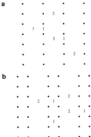
sen-sors to obscure the trees from the external sensor. Two measurements were made at each of three randomly selected positions (Fig. 1a) where each position was: (1) between trees within rows, (2) between two trees between rows, (3) diagonally between four trees be-tween rows. The software accompanying the PCA was used to calculateLand mean tilt angle (α) after Lang¯
(1986).
Interception of light by woody elements of vegeta-tion, clumping of foliage and scattering of blue light at large zenith angles are all potential sources of error in the raw reading from the PCA denoted here asLp.L
was calculated fromLpusing the relationship derived
by Hingston et al. (1998); (Eq. (2), R2=0.88) from
E. globulusstands withLranging from 1 to 6. Identi-cal relationships betweenLandLpwere obtained for
E. nitensandE. grandis(Dye, 1993; Battaglia et al., 1998).
L=1.51Lp (2)
Assuming 15% of the underestimation of L by the PCA is the result of scattering of blue light (Chen et al., 1997) we calculated the effective plant area
index,Le, for our stands from Eq. (3). The clumping
index () is the ratio ofLetoL(Black et al., 1991).
Le=1.15Lp (3)
3.3. Indirect estimation of L using hemispherical photography
Exposures were taken at a height of 1.7 m above ground level with a Nikon F90s camera equipped with a databack (Nikon MF-25), remote control shutter module (Nikon ML-3) and Sigma 8 mm, F4, fisheye lens with a clear internal filter. The focus ring was set to infinity and taped in place. The camera was mounted in a self-levelling bracket (Rich, 1989) and aligned to magnetic north. Some photographs were overexposed for use as a template to locate the boundary of the circular image on canopy photographs. Within the 10
E. globulusstands, three exposures were taken at ran-domly selected positions corresponding to positions 1, 2 and 3 (Fig. 1a). For the stands at Mandurah (low
L) and Collie (high L) photographs were taken over a greater range ofEVR within rows (position 1, Fig. 1a) to investigate the relationship betweenEVRandL
andα¯ in greater detail. No photographs were taken at position 2 (Fig. 1a) at Collie.
Initially, luminance beneath the canopy was me-tered with a handheld light meter (Capital DB3). The camera was operated in manual mode with three lens apertures (fnumber 5.6, 8.0, 11.0) and a constant shut-ter speed selected to obtainEVRof approximately−1, −2 and−3 relative to the handheld light meter. We later concluded that it was preferable to use the inter-nal light meter of the camera rather than the handheld light meter. The camera light meter was sensitive to smaller values of luminance, was more convenient to use and there was a strong linear relationship between exposure metered with the camera and with the hand-held meter (R2=0.94) which was used to deriveEVR
relative to the camera’s light meter. All subsequent references toEVRin this paper are relative to the cam-era’s light meter. The consistency of estimation ofL
obtained in variable light conditions by metering ex-posure with the camera light meter with the fisheye lens attached was tested by photographing two sites at
EVR=0 from sunset until the camera’s light meter
in-dicated a low reading and shutter speeds exceeded 4 s.
Exposures taken using Ilford XP2 ASA 400 film (suitable for the automated C41 development process) were developed by a commercial photography service. A comparison between Ilford XP2 ASA 400, Kodak T400CN ASA 400 black and white chromogenic film and Ilford Delta Professional ASA 400 pan chromatic black and white film confirmed that film type did not affect estimates ofL. In our experience, there is no improvement in contrast from using ASA 50 or ASA 100 film. ASA 5 film improves contrast but does not enable fast enough shutter speeds to freeze foliage movement due to wind (Pearcy, 1989).
Photographic negatives were scanned at 400×600
pixels as 16 tone grayscale negatives with a Nikon LS-1000 35 mm Film Scanner. Adobe PhotoShop Ver-sion 3.0 was used for image processing. The over-exposed template was used to identify the boundary of the circular canopy images. The grayscale images were converted to black and white bitmap images at 50% threshold, cropped to 400×400 pixels and saved in PCX format suitable for use in HEMIPHOT (ter Steege, 1994). A second copy of each image was twice sharpened during image processing, using the sharpen filter prior to converting to black and white. Sharpen-ing is an image compositSharpen-ing technique that increases the contrast between adjacent pixels.
HEMIPHOT was used to estimateLfrom the bitmap images after Lang (1986) based on the gap fraction at the same five zenith angles used by the PCA (7, 23, 38, 53 and 68◦; Licor, 1991). The subscript h is used to
denoteLandα¯ estimated from hemispherical photog-raphy and p to denote those estimated from the PCA. A preliminary study confirmed that there was negligi-ble difference betweenLhestimated using the method
of Lang (1986) and two other methods (Campbell, 1986; Lang, 1987). The gap fractions at the five zenith angles calculated in HEMIPHOT were recorded and used to estimateα¯h (Welles and Norman, 1991).
3.4. Estimation of diffuse light penetration beneath canopies
The diffuse non-interceptance of light (τ; Welles and Norman, 1991), calculated using the software from the PCA (Licor, 1991), was used as an esti-mate of ID to predictEVR from Eq. (1). This value
and light scattering, assuming that light scattering for all wavelengths of visible light (λ=400–700 nm) is similar to that for blue light (λ <490 nm).
3.5. Statistical treatment of data
Variation ofLhandα¯howing to sampling position,
EVRand sharpening of images, was tested using analy-sis of covariance whereEVRwas the covariate. Linear regression was used to develop relationships between
EVR,Lhandα¯hfor each stand. Separate relationships were developed for sharpened and unsharpened im-ages. These relationships were used to determine, iter-atively, theEVRthat gave agreement betweenLh
esti-mated using hemispherical photography, andLandLe
calculated fromLpusing Eqs. (2) and (3). The ‘correct’ EVR estimated by this method was compared to that
predicted from Eq. (1) using linear regression.α¯h esti-mated from sharpened and unsharpened photographs at ‘correct’EVR was compared with a pairedt-test.
3.6. Comparison of hemispherical photography and direct measurement of L
After calibrating the hemispherical photography method against the PCA, the method was tested against a direct estimate ofLobtained by destructive sampling and allometry in four stands ofE. globulus
located on the Water Authority of Western Australia effluent disposal treefarm 10 km north of Albany, Western Australia. Three stands were established with a 2 m spacing between trees within rows which were alternately 2 (comprising a ‘double row’) and 5 m apart to give an initial stand density of 1500 stems per hectare (Fig. 1b). Trees in these stands were about 13 m tall. The fourth stand was of similar spacing and density to the stands used to calibrate the hemispherical photography technique, and trees were about 11.5 m tall.
Three trees within each stand were selected to cover the range of diameters at breast height (1.3 m) over bark (Dbh) and felled. For each of the 12 trees, all live branches were removed and stratified into five groups on the basis of branch diameter (<11; 11–16; 16–22; 22–28; >28 mm). The total mass of branches in each group was measured to the nearest 0.1 kg and two sample branches were selected from each group.
These branches were immediately stripped of leaves and the wood and leaf components weighed. The area of a 200–250 g sub-sample of leaves from each branch was measured with a calibrated leaf area meter. The mean ratio of leaf area to total fresh branch mass for all branches from all sample trees in each size class was calculated and used to estimate the total leaf area of each sample tree. A logarithmic regression was devel-oped to predict total tree leaf area from tree diameter (Dbh) and used to calculate the total leaf area of each stand. The regression was corrected for proportional bias using Snowden (1991) ratio estimator for bias correction and tested for homogeneity of slope and in-tercept between stands using analysis of covariance.L
for each stand was calculated as the total area of leaves for the stand divided by the total area of the stand.
3.6.1. Indirect estimation of L by hemispherical photography
Within each of the four stands, three exposures were taken within rows (or within the 2 m spaced double rows; position 1; Fig. 1a, b) and between rows (posi-tion 2, 3) atEVR= −0.3. Photographic negatives were
scanned and processed as described earlier and all digitised images were sharpened twice.Lh was
esti-mated in HEMIPHOT and the gap fractions at the five zenith angles used to estimateα¯h after Lang (1986).
Lwas derived fromLhusing a relationship developed from the other stands. Analysis of variance was used to test the effect of sampling position within the three double-row stands onLestimated from photography. A pairedt-test was used to compareLestimated from photography and that from allometry within the three double-row stands.
4. Results
4.1. Effect of EVR, sampling position and sharpening on L andα¯estimated from hemispherical photography
Analysis of covariance indicated significant re-lationships among EVR, Lh and α¯h and significant
differences between stands. Regressions ofLhagainst EVRwere usually highly significant (P<0.001) with
Table 2
Slope and intercept of regressions of mean tilt angle (α¯h) estimated from hemispherical photography against relative exposure value (EVR)
of the form:α¯h=EVR×a+b, with adjusted correlation coefficient (R2), standard error (s.e.), statistical significance of the slope (P) and
number of observations (n)
Site Sharpened negatives Unsharpened negatives
a b R2 s.e. P n a b R2 s.e. P n
Bunbury 3.78 69.2 0.00 15.4 0.544 9 5.85 66.0 0.00 22.8 0.527 9
Busselton −0.72 79.8 0.00 12.1 0.886 9 −0.36 80.6 0.00 10.8 0.937 9
Collie 0.02 63.1 0.00 1.1 0.977 6 −0.07 62.2 0.00 3.5 0.980 5
Cowaramup 2.04 65.8 0.00 8.6 0.568 9 3.06 70.8 0.00 14.2 0.605 9
Cundinup1 1.33 77.5 0.00 9.4 0.769 9 4.61 80.7 0.09 7.5 0.224 9
Cundinup2 3.60 67.2 0.00 11.5 0.435 9 5.81 69.3 0.04 13.5 0.293 9
Grimwade 3.42 78.1 0.02 7.5 0.312 9 2.93 78.9 0.00 8.4 0.483 8
Mandurah −3.70 52.1 0.00 10.8 0.454 9 −4.10 51.8 0.00 12.1 0.456 9
Northcliffe 2.80 60.6 0.69 1.9 0.004 9 3.35 61.9 0.58 2.8 0.010 9
Scott River 1.31 61.8 0.22 1.8 0.111 9 1.72 63.2 0.33 1.9 0.063 9
(Northcliffe, Table 2).Lhincreased by 0.31–0.74 for a
one-unit reduction inEVR. Later results demonstrated
that the slope of the relationship betweenLhandEVR
increased with increasing L (R2=0.86, s.e.=0.4,
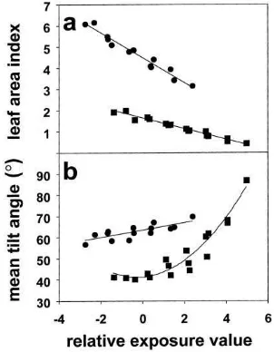
P<0.001) such that the change inLhresulting from a one-unit change inEVRwas approximately 13±0.6% of L. Detailed examination confirmed a linear rela-tionship betweenLhandEVR (Fig. 2a) but there was evidence of non-linearity in the relationship between
¯
αhandEVRat Mandurah (Fig. 2b).
Sampling position had little effect onLh(P=0.06)
but poor relationships between α¯h andEVR resulted
partly from large variation in α¯h between sampling positions within stands (P<0.001). A significant in-teraction between position and stand indicated that the effect of sampling position onα¯hwas inconsistent. In some stands,α¯hestimated between rows (positions 2 and 3; Fig. 1) was larger than that within rows (po-sition 1; Fig. 1) by up to 15◦. This could result in
an overestimate ofα¯ because twice as many measure-ments were taken from sampling positions between rows where values ofα¯hare larger. In stands, where differences betweenα¯h at position 1 and positions 2 and 3 were large,α¯ may have been overestimated by as much as 10◦.
Sharpening significantly reduced Lh (P<0.001)
at the same relative exposure and caused an average 3◦ decrease of α¯
h at ‘correct’ exposure (P=0.05).
Sharpening increased the contrast between gaps and foliage resulting in larger gaps when sharpened canopy images were converted from grayscale to
black and white, and reduced Lh estimated from
sharpened compared to unsharpened images (Fig. 3). Small gaps at large zenith angles often disappeared from unsharpened images. In canopies with large L
(Grimwade and Collie) this sometimes resulted in a gap fraction of zero for the largest zenith angle which caused excessively largeLh(e.g. 12–15) from some of the most underexposed images. These were not used for the regressions. A significant interaction between
Fig. 2. The effect of relative exposure value (EVR) on (a) leaf area
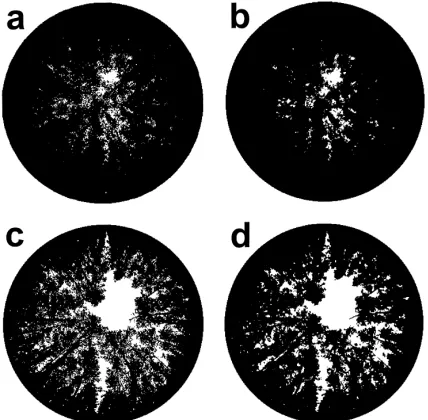
Fig. 3. Comparison of sharpened (a, c) and unsharpened (b, d), digitised images of E. globulus canopies at Collie (a, b) and Mandurah (c, d). Unsharpened images have smaller gap fractions and fewer gaps at large zenith angles compared to sharpened images.
sharpening and EVR indicated that sharpening
digi-tised images also influenced the slopes of regressions for Lh (P<0.001). Regressions of Lh on EVR
de-rived from unsharpened images always had more negative slopes than those derived from sharpened images (Table 3). Largerα¯h from unsharpened
com-Table 3
Slope and intercept of regressions of leaf area index (L) estimated by hemispherical photography against relative exposure value (EVR)
of the form:L=EVR×a+b, with adjusted correlation coefficient (R2), standard error (s.e.), statistical significance of the slope (P) and
number of observations (n) for stands ofE. globulus
Site Sharpened negatives Unsharpened negatives
a b R2 s.e. P n a b R2 s.e. P n
Bunbury −0.367 2.82 0.95 0.08 <0.001 9 −0.400 3.11 0.85 0.15 <0.001 9 Busselton −0.489 3.06 0.86 0.17 <0.001 9 −0.500 3.39 0.90 0.15 <0.001 9
Collie −0.692 4.33 0.95 0.14 0.001 6 −0.737 5.21 0.86 0.22 0.015 5
Cowaramup −0.394 3.18 0.82 0.16 <0.001 9 −0.422 3.58 0.65 0.26 0.005 9 Cundinup1 −0.390 2.67 0.81 0.14 <0.001 9 −0.474 3.15 0.68 0.24 0.004 9 Cundinup2 −0.378 3.15 0.45 0.37 0.029 9 −0.420 3.61 0.41 0.43 0.037 9 Grimwade −0.677 4.74 0.96 0.11 <0.001 9 −0.715 5.51 0.97 0.11 <0.001 8 Mandurah −0.312 1.55 0.83 0.11 <0.001 9 −0.376 1.71 0.84 0.13 <0.001 9 Northcliffe −0.452 3.51 0.87 0.18 <0.001 9 −0.604 4.22 0.85 0.26 <0.001 9 Scott River −0.314 2.74 0.68 0.18 0.004 9 −0.436 3.28 0.66 0.26 0.005 9 Fig. 4. Comparison of the relative exposure value (EVR) predicted
from Eq. (1) to obtain leaf area index (d) and effective plant area index (j) from sharpened, digitised hemispherical photographs with that estimated from the regressions in Table 3 for nine stands ofE. globulus. An outlier (Mandurah) was not included in the regression.
pared to sharpened images were also the result of the disappearance of small gaps at large zenith angles in unsharpened images.
4.2. Comparison of predicted and estimated EVR
The EVR required to obtain Le or L from
Fig. 5. Comparison of leaf area index (d) and effective plant area index (j) withLh from nine stands ofE. globulus. An outlier
(Mandurah) was not included in the regression.
hemispherical photographs but was a poor predictor of
EVRrequired to obtainLe.EVRrequired to obtainLe
from hemispherical photographs ranged from 0 to 2 while that required to obtainLranged from−1.5 to 1.
4.3. Calibration of hemispherical photography against the plant canopy analyser
Lhcalculated atEVR=0 (intercepts from equations
in Table 3) was strongly correlated withLandLe
ob-tained from the PCA (Fig. 5a, b;R2=0.93,P<0.001,
n=9). For all regressions, including those of predicted against estimatedEVR, the stand at Mandurah had a
large residual value and was excluded from the regres-sions.Lranged from 2.3–5.3 (Table 4).
Table 4
Effective plant area index (Le), leaf area index (L) and mean tilt angle (α, mean¯ ±standard error) for stands ofE. globulusin south-western
Australia measured by the Licor LAI-2000 plant canopy analyser (n=6) and hemispherical photography. For hemispherical photography, standard errors are those of the regressions used to calculateα¯h
Stand Le L α¯p α¯h (sharp) α¯h (unsharp)
Bunbury 2.0±0.05 3.0±0.06 63±1 69±15 68±23
Busselton 1.9±0.02 2.9±0.03 62±1 81±12 80±11
Collie 3.5±0.02 5.3±0.03 62±2 61±1 62±4
Cowaramup 2.0±0.03 3.0±0.05 61±5 67±9 75±14
Cundinup1 1.6±0.02 2.4±0.03 62±3 79±9 88±8
Cundinup2 2.2±0.05 3.3±0.06 61±2 67±12 74±14
Grimwade 3.3±0.07 5.0±0.09 62±5 78±8 81±8
Mandurah 1.5±0.05 2.3±0.06 62±5 62±11 58±12
Northcliffe 2.6±0.02 3.9±0.03 59±6 59±2 64±3
Scott River 1.6±0.05 2.4±0.06 69±4 65±2 67±2
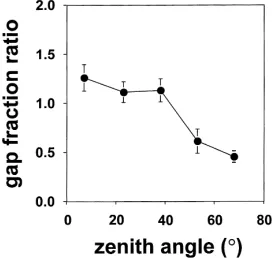
Fig. 6. The ratio of the gap fraction estimated using hemispherical photography to that measured using the Licor LAI-2000 plant canopy analyser at five zenith viewing angles in eight stands ofE. globulus. For each stand, gap fractions are means of six measurements from the PCA, and one image from each of position 1 and either 2 or 3 (Fig. 1a) taken at an exposure near that required to obtainLe.
Within a stand, the gap fraction at small zenith an-gles was usually larger from photographic images than from the PCA while the gap fraction at large zenith angles was much smaller compared to the PCA (Fig. 6). As a result, α¯p was generally less than α¯h from either sharpened or unsharpened photographic images (Table 4).
4.4. Comparison of hemispherical photography and direct estimation of L in highly clumped stands
Lhof the single row stand ofE. globulus(Fig. 1a;
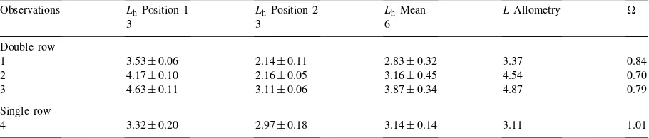
Table 5
Leaf area index (L) measured by allometry and hemispherical photography (mean±s.e.) and clumping index () of four stands ofE. globulusnear Albany, Western Australia. Three stands were planted in closely spaced double-rows and one in evenly spaced single rows. The positions refer to Fig. 1a, b.is calculated as the ratio of meanLh toLfrom allometry
Observations Lh Position 1 Lh Position 2 Lh Mean LAllometry
3 3 6
Double row
1 3.53±0.06 2.14±0.11 2.83±0.32 3.37 0.84
2 4.17±0.10 2.16±0.05 3.16±0.45 4.54 0.70
3 4.63±0.11 3.11±0.06 3.87±0.34 4.87 0.79
Single row
4 3.32±0.20 2.97±0.18 3.14±0.14 3.11 1.01
the stands planted in double rows (Fig. 1b; stands 1–3),
Lh underestimatedL by 16–30% (Table 5).Lh
mea-sured beneath the double rows (position 1; Fig. 1b) was 1.5–2 times greater than that measured between the double rows (position 2; Fig. 1b;P<0.001). Lh
measured only beneath the double rows agreed well with directly measuredL.
5. Discussion
This study revealed that hemispherical photography, a technique which is markedly cheaper than alterna-tives, can be used to obtain estimates of leaf area in-dex (L) as reliable as those from the LAI-2000 plant canopy analyser in plantations of E. globulus. Lh is
influenced by photographic exposure and stand struc-ture but consistent measurements of Lh can be
ob-tained under varying light conditions by metering light with a camera’s light meter with the fisheye lens at-tached. Lh estimated at a constant photographic
ex-posure is strongly correlated withLdetermined from other methods such that, once calibrated, Lh can be
used to predictL.
Lh is larger at smallerEVRbecause the calculated gap fraction decreases as images become darker with greater underexposure. The rates of increase ofLhwith decreasingEVRin this study (0.3–0.7) were similar to that found inP. menziesii(c. 0.6; Chen et al., 1991) and indicates that variations of photographic exposure can greatly affect estimates ofL. The rate of increase of Lh withEVR was proportional toL such that a 1
stop change of exposure changedLhby approximately
13% ofL. The rate of change ofLhwith photographic
exposure as a proportion of Lwas so consistent that
it may be possible to use this relationship to predict
L. For such a relationship to be generally applicable it would need to be tested in vegetation where the value ofLeis more certain because the effect of exposure on Lhis related toLe, rather thanL. The variation ofLh
that can be expected from varying exposure is of sim-ilar magnitude to the total accumulated errors associ-ated with both indirect (10–30%) and direct (<25%) methods (Chen et al., 1997).
Strong correlation between the predicted and mea-sured exposure required to correctly estimateLorLe
from hemispherical photographs supports the proposal of Chen et al. (1991) that the ‘correct’ exposure to ob-tain good contrast between sky and foliage decreases with increasing canopy density. However, the ‘cor-rect’ exposure to obtain estimates ofLepredicted from
Eq. (1) underestimated the measured exposure by 2.5 stops. This may result in part from variation between light meters (Wagner, 1998) but the much better agree-ment between predicted exposure and that required to estimateLfrom photographs suggests instead thatLe
may be more similar toL than indicated in Eq. (3). This implies that much of the underestimation ofLby the PCA in evenly spaced stands ofE. globulusresults from scattering of blue light rather than foliage clump-ing. Using Eq. (1) to predict correct exposure would have resulted in an over-estimation ofLby up to 10% because of the 0.8 stop difference between predicted and actual correct exposure.
Scattering of light generally results in 8–19% underestimation by the PCA of Le in conifers but
eucalypt foliage would also have larger scattering coefficients than conifers. This could result in greater underestimation ofLein eucalypt and deciduous
for-est by the PCA. Thomas and Barber (1974) measured reflectance of photosynthetically active radiation (PAR) of leaves ofE. urnigera. Reflectance for PAR ranged from 13% for glossy green leaves, similar to adult leaves ofE. globulus, up to 30% for glaucous leaves, similar to juvenile foliage of E. globulus. In comparison, reflectance of PAR by old foliage of P. menziesiiranged from 6 to 10% (Jarvis et al., 1976). The size of the PCA correction factors for species such as E. globulus,E. grandis and E. nitens (Dye, 1993; Battaglia et al., 1998; Hingston et al., 1998) may be increased by the glossy adult foliage of these three species and, except forE. grandis, any glaucous juvenile foliage that may be present (Brooker and Kleinig, 1996). Numerous other studies have found underestimation ofLe by the PCA of 10–40% in
ev-ergreen and deciduous broadleaf species which are not noted for foliage clumping (e.g.Wang et al., 1992; Martens et al., 1993; Eschenbach and Kappen, 1996; Strachan and McCaughey, 1996). Large underestima-tion of Le by the PCA might also be expected for stands ofPiceaspp. with large reflectance in the blue waveband (Jarvis et al., 1976).
If the objective of sampling is solely to obtain an estimate of L (and not an accurate distribution of gap fractions) then as an alternative to attempting to predict ‘correct’ exposure, L can be estimated from empirical relationships between Lh measured at the
sameEVR beneath the canopy, regardless of canopy
density. This approach is convenient as it does not require the operator to return outside the canopy to determine the correct exposure under changing light conditions. In climates, where clear skies are com-mon and most measurements are made at sunrise and sunset, light conditions change rapidly and it is impractical to regularly re-meter exposure outside the canopy. The time required for metering expo-sure also reduces the number of stands that can be sampled. Allometry or another calibrated indirect method is necessary to determine the relationship between Lh and L, but even if the ‘correct’
expo-sure were used, the relationship between Le and
L would need to be determined by similar
meth-ods, assuming that the clumping index is unknown. The need for destructive sampling appears to negate
one of the main advantages of indirect methods for estimatingL. However, indirect methods still have one great advantage over allometric methods in that indi-rect measurements can be made and their relationship toL determined either retrospectively when the op-portunity and resources for destructive sampling are available, or in similar vegetation to that being studied. Once calibrated for a vegetation type, indirect methods should provide reliable results whereas allometric methods often remain site-and age-specific. In cli-mates, where uniform overcast skies persist for much of the day and light conditions change slowly, meter-ing of exposure outside the canopy may be practical. The difference between the gap fraction measured at large zenith angles by the PCA and that measured with photographs is also consistent with more scattering of blue light near the horizon and is further evidence that much of the underestimation of L inE. globulus by the PCA may result from light scattering rather than foliage clumping. Evenly spaced crowns in a closed or nearly closed canopy generally meet the assumption of randomly distributed foliage (Chen and Cihlar, 1996), hence, it is likely that there was little foliage clumping in the stands measured with the PCA. Agreement of
Lmeasured between and within rows of these stands further suggests that the foliage was not significantly clumped at the crown level.
The small gap fractions derived from photographic images at large zenith angles compared to the PCA may also result from the loss of small gaps when the images were converted from grayscale to black and white. We attempted to reduce this effect by sharp-ening the images during processing. Sharpsharp-ening of images increased the overall gap fraction by increas-ing the size of gaps in foliage and preventincreas-ing small gaps at large zenith angles from disappearing when images were converted from grayscale to black and white (Fig. 3). Similarly, Chen et al. (1991) found that increasing the contrast during processing of im-ages from ASA 100 film gave similar results to those obtained from high contrast ASA 5 film. The greater sensitivity ofLh to exposure in unsharpened images is further argument for sharpening of images prior to analysis.
underestimated at large zenith angles owing to re-duced sky brightness. Wagner (1998) observed that, even when overexposed by 3 stops, sky brightness in photographs decreased rapidly at zenith angles larger than 70◦. Fournier et al. (1997) observed that
simu-lated gap fractions in the BOREAS study sites agreed well with those obtained from photographs between zenith angles of 20–70◦. The larger gap fraction at
the 7◦ zenith angle obtained from photography in
our study probably indicates some scattering of light from high foliage, even under relatively uniform, dif-fuse light conditions. This phenomenon would also explain the poor agreement at zenith angles less than 20◦ observed in the BOREAS sites (Fournier et al., 1997). However, this effect is small compared to large differences observed at large zenith angles. It may be preferable to avoid measuring gap fractions at zenith angles larger than 70◦ with hemispherical
photography and at zenith angles larger than 50◦with
the PCA. If much of the underestimation ofLby the PCA results from blue light scattering then the gap fraction ratios (Fig. 6) are overestimates because they are based on photographs that agreed withLe. Using photographs that agreed withL would have resulted in ratios closer to one for the smaller zenith angles but increased the difference between gap fractions from photographs and the PCA at large zenith angles. Good agreement betweenα¯hfor the 10E. globulus
stands (68.7◦±2.5 s.e.) with those obtained from
di-rect measurements for another species noted for near vertical foliage, E. regnans (68◦±10 s.d.), from a
range of Eucalyptus saplings (70–77◦) and with α¯ h
obtained for a range of eucalypt forests in eastern Australia (60–80◦) suggests that the gap fraction
tained from photographs is more realistic than that ob-tained from the PCA (Ashton, 1976; Anderson, 1981; King, 1997). Chen et al. (1991) concluded that the gap fraction distribution from photographs was unrealistic but their conclusion assumed that blue light scatter-ing made a negligible contribution to the gap fraction distribution obtained from the PCA. The difference betweenα¯h estimated at different sampling positions within stands and at different stands indicates that the structure of the stand influencesα¯h independently of the foliage angle distribution, and that estimates ofα¯
derived from any zenith angle range, with either the PCA or hemispherical photography, should be inter-preted with caution.
In plantations with closely spaced double rows and large inter-row gaps (Fig. 1b), foliage clumping at the crown level appeared to cause significant underesti-mation of L: ranged from 0.70 to 0.84 for these stands (Table 5). Chen and Cihlar (1996) found that for a stand obtained from indirect light interception methods was influenced by stand density,Leand tree
height. As tree height (or canopy depth) increases, and as gap size decreases, the zenith angle at which large gaps disappear decreases. Large errors in estimation ofL may result from optical methods in stands with ‘extreme’ architecture. In the double-row stands, the trees were several metres shorter than in the stands where the photographic technique was calibrated and the gaps were much larger owing to the spacing of the rows.was probably larger in these stands than in even the sparsest single row stands. This resulted in significant differences betweenLhmeasured within
and between double rows.Lh measured only beneath
the double rows was within 5–8% ofLderived from allometry. This could be the result of the large gaps between rows being removed from view by position-ing the camera directly beneath the rows of trees and suggests that even in stands with ‘extreme’ architec-tureL could be indirectly estimated with reasonable accuracy if the camera can be positioned to remove large gaps from view.
6. Conclusions
This study has shown that in young stands of
Eucalyptuswith foliage evenly distributed through the canopy, hemispherical photography can reliably esti-mate leaf area index (L), once the technique has been calibrated. Hemispherical photography is cheaper and simpler to use than the PCA which has the further disadvantage that scattering of blue light can cause significant underestimation ofL. Estimates of leaf area from photographs (Lh) are sensitive to photographic exposure but ‘correct’ exposure can be reasonably predicted from exposure metered outside the canopy. If the main objective is to obtain estimates ofL and not to describe the full architecture of the canopy, we recommend the use of empirical relationships be-tweenLhandL. Whether exposure is metered outside
the relationship betweenL and eitherLh or effective
plant area index.
Underestimation ofLby the PCA appears to be as-sociated mainly with scattering of blue light in single row stands ofE. globulus. In stands with ‘extreme’ ar-chitecture, indirect, light interception methods can be subject to large errors as a result of foliage clumping at levels above the shoot. In such stands ofE. globu-luswe estimatedto be between 0.70 and 0.84. Po-sitioning the camera to remove large gaps from direct view may allow accurate estimates ofLeven in these stands.
7. List of symbols and abbreviations
ASA American Standards Association film
speed
Dbh tree diameter at breast height (1.37 m; m) EVR relative exposure value (dimensionless)
ID diffuse radiation penetration
(dimensionless)
L leaf area index (dimensionless)
Le effective plant area index (dimensionless)
Lh plant area index estimated from
hemispherical photography (dimensionless)
Lp raw value of plant area index from the
PCA (dimensionless)
PCA plant canopy analyser (Licor LAI-2000)
¯
α mean tilt angle (degrees)
¯
αh mean tilt angle estimated from
hemispherical photography (degrees)
¯
αp mean tilt angle estimated from the
PCA (degrees)
λ wavelength of light (nm)
τ diffuse radiation non-interceptance
(dimensionless)
foliage clumping index at all levels
(dimensionless)
Acknowledgements
The authors wish to acknowledge Bunning’s Tree-farms Pty. Ltd., the Department of Conservation and Land Management, Western Australia and the Water Authority of Western Australia for permission to use
experimental sites and the Australian Research Coun-cil for financial assistance. We thank Paul Dignan for advice on image analysis and HEMIPHOT, Michael Kemp and Lachlan Ingram for technical assistance, and Andrew Stilwell for valuable suggestions. Craig Macfarlane is supported by an Australian Postgraduate Award with Stipend and a Jean Rogerson Postgradu-ate Scholarship. Michael Coote is supported by a Wa-ter Authority of WesWa-tern Australia/UWA Scholarship. We also thank one anonymous reviewer for valuable advice on analysis of the data.
References
Anderson, M.C., 1981. The geometry of leaf distributions in some south-eastern Australian forests. Agric. Meteor. 25, 195–205. Ashton, D.H., 1976. The development of even-aged stands of
Eucalyptus regnansF. Meull. in Central Victoria. Aust. J. Bot. 24, 397–414.
Battaglia, M., Cherry, M.L., Beadle, C.L., Sands, P.J., Hingston, A., 1998. Prediction of leaf area index in eucalypt plantations — effects of water stress and temperature. Tree Physiol. 18, 521–528.
Black, T.A., Chen, J.M., Lee, X., Sagar, R.M., 1991. Characteristics of short-wave and long-wave irradiances under a Douglas-fir stand. Can. J. For. Res. 21, 1020–1028.
Brooker, I., Kleinig, D., 1996. Eucalyptus: An Illustrated Guide to Identification. Reed Books, Port Melbourne.
Campbell, G.S., 1986. Extinction coefficients for radiation in plant canopies calculated using an ellipsoidal inclination angle distribution. Agric. For. Meteor. 36, 317–321.
Canham, C.D., Denslow, J.S., Platt, W.J., Runkle, J.R., Spies, T.A., White, P.S., 1990. Light regimes beneath canopies and tree-fall gaps in temperate and tropical forests. Can. J. For. Res. 20, 620–631.
Chen, J.M., 1996. Canopy architecture and remote sensing of the fraction of photosynthetically active radiation absorbed by boreal conifer forests. IEEE Trans. Geosci. Remote Sens. 34, 1353–1368.
Chen, J.M., Black, T.A., Adams, R.S., 1991. Evaluation of hemispherical photography for determining plant area index and geometry of a forest stand. Agric. For. Meteor. 56, 129–143. Chen, J.M., Cihlar, J., 1996. Retrieving leaf area index of
boreal conifer forests using Landsat TM images. Remote Sens. Environ. 55, 153–162.
Chen, J.M., Rich, P.M., Gower, S.T., Norman, J.M., Plummer, S., 1997. Leaf area index of boreal forests — theory, techniques and measurements. J. Geophys. Res. 102 (D24), 29429–29443. Dunin, F.X., Mackay, S.M., 1982. Evaporation of eucalypt and coniferous forest. In: The First National Symp. on Forest Hydrology, 11–13 May, 1982. Melbourne, pp. 18–25. Dye, P., 1993. A Report on a Visit to Australia by Dr. Peter Dye.
Eschenbach, C., Kappen, L., 1996. Leaf area index determination in an alder forest: a comparison of three methods. J. Exp. Bot. 47, 1457–1462.
Fournier, R.A., Rich, P.M., Landry, R., 1997. Hierarchical characterization of canopy architecture for boreal forest. J. Geophys. Res. 102 (D24), 29445–29454.
Gholz, H.L., Ewel, K., Teskey, R.O., 1990. Water and forest productivity. For. Ecol. Manage. 30, 1–18.
Gower, S.T., Norman, J.M., 1991. Rapid estimation of leaf area index in conifer and broad-leaf plantations. Ecology 72, 1896– 1900.
Grimm, T., Grimm, M., 1997. The Basic Book of Photography. Plume, New York.
Hingston, F.J., Galbraith, J.H., Dimmock, G.M., 1998. Application of the process-based model BIOMASS toEucalyptus globulus subsp. globulus plantations on ex-farmland in south western Australia I. Water use by trees and assessing risk of losses due to drought. For. Ecol. Manage. 106, 141–156.
Jarvis, P.G., James, G.B., Landsberg, J.J., 1976. Coniferous forest. In: Monteith, J.L. (Ed.), Vegetation and the Atmosphere, vol. 2. Academic Press, London, pp. 171–240.
King, D.A., 1997. The functional significance of leaf angle in Eucalyptus. Aust. J. Bot. 45, 619–639.
Lang, A.R., 1986. Leaf area and average leaf angle from transmittance of direct sunlight. Aust. J. Bot. 34, 349–355. Lang, A.R., 1987. Simplified estimate of leaf area index from
transmittance of the sun’s beam. Agric. For. Meteor. 41, 179– 186.
Licor, 1991. Plant Canopy Analyser Instructional Manual. LI-COR Inc., Lincoln, Nebraska, USA.
Lieth, H., 1975. Modeling the primary productivity of the world. In: Lieth, H., Whittaker, R.H. (Eds.), Primary Productivity in the Biosphere. Springer, New York, pp. 237–263.
Martens, S.N., Ustin, S.L., Rousseau, R.A., 1993. Estimation of tree canopy leaf area index by gap fraction analysis. For. Ecol. Manage. 61, 91–108.
Norman, J.M., Campbell, G.S., 1989. Canopy structure. In: Pearcy, R.W., Ehleringer, J.R., Mooney, H.A., Rundel, P.W. (Eds.), Plant Physiological Ecology. Field Methods and Instrumentation. Chapman and Hall, London, UK, pp. 301–326.
Pearcy, R.W., 1989. Radiation and light measurements. In: Pearcy, R.W., Ehleringer, J.R., Mooney, H.A., Rundel, P.W. (Eds.), Plant Physiological Ecology. Field Methods and Instrumentation. Chapman and Hall, London, UK, pp. 97–116.
Rich, P.M., 1989. A Manual for Analysis of Hemispherical Canopy Photography. Los Alamos National Laboratory Report LA-11733-M.
Rich, P.M., 1990. Characterizing plant canopies with hemispherical photographs. Remote Sens. Rev. 5, 13–29.
Rich, P.M., Chen, J., Sulatycki, S.J., Vashisht, R., Wachspress, W.S., 1995. Calculation of Leaf Area Index and Other Canopy Indices from Gap Fraction: A Manual for the LAICALC Software. Kansas Applied Remote Sensing Program Open File Report.
Snowden, P., 1991. A ratio estimator for bias correction in logarithmic regressions. Can. J. For. Res. 21, 720–724. Stenberg, P., 1996. Correcting LAI-2000 estimates for the clumping
of needles in shoots of conifers. Agric. For. Meteor. 79, 1–8. Strachan, I.B., McCaughey, J.H., 1996. Spatial and vertical leaf
area index of a deciduous forest resolved using the LAI-2000 plant canopy analyser. For. Sci. 42, 176–181.
ter Steege, H., 1994. Tropenbos Document 3. Hemiphot: A Programme to Analyze Vegetation Indices, Light and Light Quality from Hemispherical Photographs. The Tropenbos Foundation, Wageningen, The Netherlands.
Thomas, D.A., Barber, H.N., 1974. Studies on leaf characteristics of a cline of Eucalyptus urnigera from Mount Wellington, Tasmania. II Reflection, transmission and absorption of radiation. Aust. J. Bot. 22, 701–707.
Unwin, D.M., 1980. Microclimate Measurement for Ecologists. Academic Press, London.
Wagner, S., 1998. Calibration of grey values of hemispherical photographs for image analysis. Agric. For. Meteor. 90, 103– 117.
Wang, W.S., Miller, D.R., Welles, J.M., Heisler, G.M., 1992. Spatial variability of canopy foliage in an oak forest estimated with fisheye sensors. For. Sci. 38, 854–865.
Waring, R.H., 1983. Estimating forest growth and efficiency in relation to canopy leaf area. Adv. Ecol. Res. 13, 327–354. Watson, D.J., 1958. The dependence of net assimilation rate upon
leaf area index. Ann. Bot. Lon. New Ser. 22, 37–54. Welles, J.M., Cohen, S., 1996. Canopy structure measurement by
gap fraction analysis using commercial instrumentation. J. Exp. Bot. 47, 1335–1342.