Trend-stationarity, difference-stationarity, or neither:
further diagnostic tests with an application to
U.S. Real GNP, 1875–1993
Paul Newbold
a,*, Stephen Leybourne
a, Mark E. Wohar
baDepartment of Economics, University of Nottingham, Nottingham NG7 2RD, UK b
Distinguished Enron Professor, Department of Economics, University of Nebraska at Omaha, Omaha, NE 68182, USA
Received 4 May 1999; received in revised form 24 July 2000; accepted 28 July 2000
Abstract
Recent studies have found evidence suggesting that US Real GNP is trend-stationary over a long period of time. This paper presents an analysis of US real GNP over the period 1875–1993 and finds that neither simple trend-stationary nor difference-stationary specifications are adequate. We find very strong evidence against a common fixed trend-stationary representation in the periods 1875–1929 and 1950 –1993. If a choice between difference-stationarity and trend-stationarity must be made, we prefer the former, as it implies less stringent assumptions. Our analysis provides a new diagnostic testing procedure that practitioners can employ when faced with conflicting results concerning trend-station-ary versus difference-stationtrend-station-ary specifications. © 2001 Elsevier Science Inc. All rights reserved.
JEL classification:C22; C51
Keywords:Unit root; Trend-stationary; Difference-stationary
1. Introduction
Prior to the publication of the Nelson and Plosser (1982) paper it was common to model real GNP as transitory deviations about a deterministic trend. With the publication of the Nelson-Plosser paper, the tide changed, and US real GNP (henceforth RGNP) was deemed
* Corresponding author. Tel.:1011-44-115-951-5392; fax:1011-44-115-951-4159. E-mail addresses:[email protected] (P. Newbold).
to contain a nonstationary stochastic trend (random walk) and hence, it was argued, should be modeled as a first difference stationary (DS) process. Empirical studies by Stock and Watson (1986), Perron and Phillips (1987), Campbell and Mankiw (1987), Evans (1989) and most recently, Murray and Nelson (2000), have failed to reject the null of a unit root in RGNP (supporting a DS model) for post-World War II quarterly RGNP.
Other studies, using longer spans of data on RGNP, have argued against the apparent stochastic trend (or DS) nature of RGNP, in favor of a trend stationary (TS) process. For example, using Dickey-Fuller tests,1 Diebold and Senhadji (1996) and Cheung and Chinn (1997), analyzing US RGNP beginning in the 1870s, found very strong evidence against unit autoregressive roots, and, by implication, in favor of TS.2 Diebold and Senhadji (1996) suggested that, in part, this outcome could be attributed to the additional power resulting from a larger sample, and also that the Nelson-Plosser findings were driven by the special circumstances in an important subperiod of their series.
As there is still considerable debate about the time series nature of RGNP, it seems appropriate to ask how robust are these results to various factors, including sample period and testing techniques. The purpose of this paper is to critically examine the conflicting results concerning the data generating process for RGNP over the period 1875–1993, a period chosen so as to make our results comparable with previous studies. In particular, this paper provides a new diagnostic testing procedure that practitioners can employ when faced with conflicting results concerning TS vs. DS specifications. Specifically, we first utilize a moving Dickey-Fuller (parametric bootstrap) test, based on standard deviations, to test the adequacy of a TS specification versus a DS specification. Second, we combine this test with multistep ahead forecasts and ratios of mean squared errors to provide guidance in choosing between alternative specifications.
2. Uncertainty about the unit root hypothesis
As argued by Christiano and Eichenbaum (1990), and more technically by Faust (1996), every DS process is arbitrarily close to some TS process, and vice versa. Cochrane (1991) has identified a similar observational equivalence between a TS process and a DS process when the variance of the innovation is small. Statistical distinction between such processes is practically impossible, although it is practically important for inference, modeling, and forecasting at long-run horizons. However, given limited amounts of data, parsimoniously parameterized TS and DS models achieved in practice can be quite distinct.
It is important to be precise about the null and alternative hypotheses of the traditionally used Dickey-Fuller test. In the present context, the null hypothesis is that a time series is
stationary after, but only after, first differencing. The alternative hypothesis is TS, generally about a linear trend, in levels. The emphasis on stationarity in differences under the null is crucial, so that this hypothesis is best stated as DS. Rejection of the null is then rejection of DS.3Although the Dickey-Fuller test is designed to have power against TS, strong rejections of the null hypothesis can occur as a result of departures from DS other than TS. Similarly, failure to reject the null of DS can be a manifestation of phenomena other than a DS data generating process. There are a number of possibilities.4
First, Dickey-Fuller tests are based on the prior fitting of relatively low order autoregres-sions. It follows that these tests are valid only if the true generating process is a low order autoregression, or can be adequately approximated by such. However, for some time series, the true generating process will incorporate a moving averagecomponent.5 Such a compo-nent arises, for example, from simple models where an outcome is viewed as the sum of permanent and transitory components. It is well known (Schwert, 1989; Agiakloglou and Newbold, 1992) that large moving average components generate spurious rejections by Dickey-Fuller tests. Ng and Perron (1995) prove that use of particular criteria for selecting autoregressive order in Dickey-Fuller tests leave the asymptotic null distribution undisturbed for a range of generating models involving moving average terms.6While this seems about the best that can be done, Agiakloglou and Newbold (1996) demonstrate for typical sample sizes, that although the spurious rejection problem is somewhat alleviated, it may be far from cured.
is the sum of an integrated component with drift and an occasional large transitory compo-nent will generate data in finite samples that is difficult to distinguish from a trend stationary process with a trend break. They report that purely transitory disturbances can cause rejection of the unit root null hypothesis and spurious results indicating that there has been a permanent shift in the level.
Third, it is also the case that outliers (Franses and Haldrup, 1994) or structural breaks (Leybourne, Mills and Newbold, 1998) can induce spurious rejections by Dickey-Fuller tests. This issue was raised by Nelson and Murray (2000) in discussing tests for unit roots in RGNP. Lengthening the span of data increases the possibility of major structural changes. Failure to account for such structural changes will bias unit root tests. For example, Leybourne, Mills and Newbold (1998) found results converse to those of Perron (1989). They show that when a series is generated by a process that is I(1), with an early (but not late) break, application of the Dickey-Fuller test will lead to spurious rejection of the unit root null hypothesis. These results suggest that the application of the Dickey-Fuller tests will yield misleading results when applied to data that have a structural break early in the series. One important implication of these findings is that studies that justify using longer spans of data on the grounds of increasing the power of the tests and more precise estimates, can lead to erroneous findings if the early data contains a structural break.
In our view, statistical tests of unit roots will almost inevitably be based explicitly or implicitly on models that are drastic simplifications of the underlying generating process. It is simply impossible, given available data, to simultaneously contemplate models that are more highly parameterized than the typical parsimonious forms, including possible moving average terms, and allow for the possibility of both outliers and structural breaks of unknown form and type, occurring at unknown points in time. Whether the simplified structures on which the tests are necessarily based are helpful or misleading is difficult to anticipate in any application.
3. US real GNP, 1875–1993
In the remainder of this paper we present statistical evidence against the TS hypothesis, while accepting that this does not imply DS as a likely alternative. To allow comparison with earlier studies, we employ the same series as Diebold and Senhadji (1996) in our empirical analyses. These authors used four series, GNP-BG, GNP-R, GNP-BGPC, GNP-RPC based on whether measures from Balke and Gordon (1989) or Romer (1989) were used or whether RGNP was expressed in per capita form. In all cases the logarithmic transformation was applied.
by considering autoregressive-moving average, ARMA(p,q) models as possible generators of the series of first differences.
Ifytdenotes the logarithm of RGNP, these models are of the form
~12f1L2. . .2fpLp!~Dyt2b!5~12u1L2. . .2uqLq!et (1)
where L is the lag operator and et zero-mean white noise. To ensure replicability of our results, the orders (p,q) were chosen through the Schwarz Bayesian Criterion (SBC), rather than judgmental methods. This criterion is known to yield consistent estimators of (p,q) when the true model is in the contemplated set (Hannan, 1982). The parameters of (1) were estimated through full maximum likelihood, using a GAUSS subroutine, and all combina-tions of orders withp1q#7 were estimated. For all four time series, SBC selected a model whose estimated parameters implied a unit moving average root, indicating overdifferencing in the model (1).9
These results reinforce the Diebold-Senhadji evidence against difference-stationarity, and moreover do so with no prior assumption of a pure autoregressive generating model. However, our evidence is not entirely conclusive, as it is well known [Cryer and Ledolter (1981), Shephard and Harvey (1990), and Davis and Dunsmuir (1996)] that maximum likelihood estimates can fall on the boundary of the invertibility region in the absence of a unit moving average root. Nevertheless, it is difficult to see how an investigator can proceed with a DS model of the form (1) in these circumstances. If that investigator is committed to linear models with fixed parameters, the next step would be to consider stationarity around a linear trend. We applied the test of Leybourne and McCabe (1994, 1996), in which the null hypothesis is TS and the alternative is DS. In no case was TS rejected at the usual significance levels [see Cheung and Chinn (1997), for a similar finding over almost the same period].
The apparently strong evidence of TS over a period of 119 years is somewhat perplexing, as many analyses using post-World War II quarterly RGNP have supported a DS model. Moreover, Dickey-Fuller tests applied to the annual series over the period 1950 –1993 failed to yield strong evidence against DS.10The test statistics are the t-ratios associated with the least squares estimate ofg in the regression
Dyt5a 1 bt1gyt211
O
j51
k
djDyt2j1et (2)
In line with the recommendation of Ng and Perron (1995), we chose k in (2) through general-to-specific testing at the 10%-level, with a maximum possible value of 5. The resulting test statistics are 21.993 for RGNP and 22.516 for RGNP per capita. Neither is significant at the 10%-level. Nelson and Murray (1997) present further tests which, on balance, failed to provide strong evidence of trend-stationarity in the postwar period.
longer period.12The true DGP may have changed between the postwar and prewar periods. A third possibility is that the existence of structural breaks leads to spurious results.
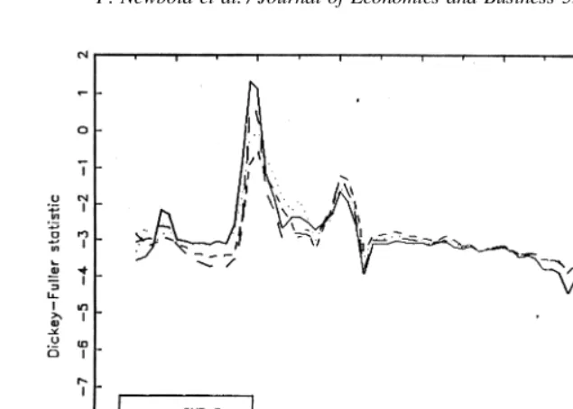
To explore these possibilities, and assist in sorting out some of the complexities mentioned above when attempting to test DS against TS specifications, we develop a new diagnostic methodology. First, we applied the Dickey-Fuller test (lag 55), implemented precisely as described in the previous paragraph, to all blocks of 44 consecutive observations, beginning with 1875–1918, and ending with 1950 –1993, giving 76 Dickey-Fuller statistics. The results for the four RGNP series are graphed in Fig. 1. Two notable features of these graphs are: i) two periods of extreme volatility and ii) a very wide range for the test statistics. Intuition would suggest that patterns of this kind are very unlikely to be found for (trend) stationary generating processes. Trend stationary processes would yield much larger and stable Dickey-Fuller values. Indeed, thoughtful graphical inspection can often alert one to at least the most extreme problems.
To check this intuition, we carried out a simulation experiment, in which series of 119 observations were generated from the second order autoregressive TS models given in Table 1 of Diebold and Senhadji (1996).13Moving Dickey-Fuller statistics, based on 44 observa-tions, precisely as in Fig. 1, were calculated. For each of the 2000 replicaobserva-tions, the standard deviations and ranges of the 76 Dickey-Fuller statistics were compared with the correspond-ing values from the actual time series. In the terminology of Tsay (1992), this can be viewed as a parametric bootstrap specification test of the TS model. The p-values for these tests are shown in Table 1.14For example, in only 1.6% of replications was the standard deviation of the moving Dickey-Fuller statistics greater than that for the actual GNP-R data. Put differ-ently, 98.4% of the 2000 replicated standard deviations (of the 76 Dickey-Fuller statistics) had values less than those of Fig. 1. Stated another way, if the actual data were TS then one
would obtain the actual moving Dickey-Fuller statistic pattern or one more extreme only 1.6% of the time (for GNP-R). This means that one would reject the null of TS at the 1.6% level with these large values.
The moving Dickey-Fuller (parametric bootstrap) tests which we offer here, based on standard deviations, suggest that the adequacy of the TS specifications can be rejected at significance levels between 1.6% (for GNP-R) and 3.5% (for GNP-BGPC), while the tests based on ranges generate rejections at levels of practically zero. It is for this reason that, though we concur with the conclusion of Diebold and Senhadji (1996) and others, that DS over the whole 119-year period is unlikely, we are evenmoreskeptical about the hypothesis of TS over this period.
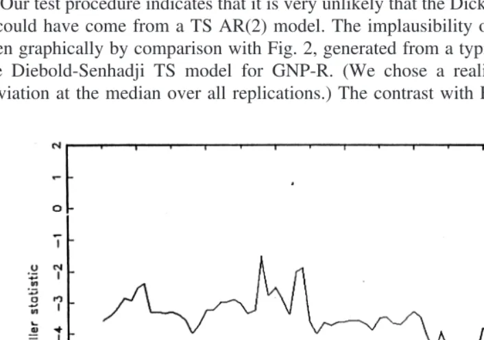
Our test procedure indicates that it is very unlikely that the Dickey-Fuller statistics of Fig. 1 could have come from a TS AR(2) model. The implausibility of Fig. 1 under TS can be seen graphically by comparison with Fig. 2, generated from a typical series simulated from the Diebold-Senhadji TS model for GNP-R. (We chose a realization giving a standard deviation at the median over all replications.) The contrast with Fig. 1 is quite stark.
Table 1
p-values of parametric bootstrap tests of trend-stationary models, based on moving Dickey-Fuller tests
GBP-R GNP-RPC GNP-BG GNP-BGPC
Std. deviation 0.016 0.028 0.025 0.035
Range 0.000 0.000 0.004 0.000
This bootstrap method is not without limitations. One might argue that in order to test for power we should also reverse the null to be DS and redo the test. But issues of power are more of a concern when one is not able to reject the null of TS when DS is true. In the case whereb(i.e. the likelihood of not rejecting TS, given that DS is true) is large, the power of the test will be low.15Reversing things and generating moving Dickey-Fuller tests from a DS series, would yield p-values that are very large. That is, the likelihood of getting the observed actual series would be very high in this case. This means that the likelihood of not rejecting TS, given that DS is true (b), would be small. With a small value ofbthe power of the test would be high.16Regardless of the above, since our objective is to investigate the degree of evidence against TS, repeating our simulation, replacing the current null of TS with DS, would yield little as Diebold and Senhadji (1996) have already shown there is evidence against the DS model.
Although the earlier Dickey-Fuller tests and ARMA models clearly cast doubt on the DS specification over the 119 years of data, from the moving Dickey-Fuller tests it appears equally unlikely that the series over 119 years was generated from a TS model.17 The progression over time of the graphs of Fig. 1 is interesting and suggestive. As observations from the early 1930s enter towards the end of a block of data, we find Dickey-Fuller statistics close to zero, suggesting, on the surface, virtually no evidence against DS. If the true process was TS, we could view this as reflecting the finding of Perron (1989) of very low power of Dickey-Fuller tests in the presence of a structural break. By contrast, when this possible break is early in the block, the Dickey-Fuller statistics are very far from zero. Leybourne, Mills and Newbold (1998) have shown that, if the true generating process is DS with an early (but not late) break, spurious rejections by Dickey-Fuller tests will frequently occur.
Our own view is that the series of RGNP over the whole period 1875–1993 are neither trend-stationary nor difference-stationary. Indeed, a casual inspection of a graph of the data would make this point transparent (see Figs. 5 and 6, discussed in the next section). The aberrant behavior of the time series over the period 1930 –1949 is a strong factor in arriving at this conclusion. The behavior of the series over a period of approximately twenty years, from 1930 –1949, is quite different from anything previously or subsequently. It is simply unreasonable to believe that the same generating regime operated over this period as elsewhere. As we have noted, it is precisely this period that generates the peculiar graphs of Fig. 1.
4. US real GNP, 1875–1929 and 1950 –1993
It is possible to inquire into the plausibility of TS between 1875 and 1993 while discounting the experience of 1930 –1949. This would still require the existence of a fixed trend line over the whole period, and presumably the same second moment structure around that line before 1930 and after 1949. To investigate this possibility, we established a TS regime by fitting to the 1875–1929 period TS models from the ARMA(p,q) class given below.
~12f1L2. . .2fpLp!~yt2a 2 bt!5~12u1L2. . .2uqLq!et (3)
As before (p,q) were selected through SBC, which yielded afirst-orderautoregression for all four series (GNP-BG, GNP-R, GNP-BGPC, GNP-RPC).18We then used these fitted models to generate forecasts from base years 1950, 1951, . . . , 1992. This yields 43 one-year-ahead forecasts, 42 two-year-ahead forecasts, and so on, that can be compared with the observed true values of the series. To give a basis for comparison, we also fitted DS models of the form (1) to the 1875–1929 data. In all cases, the random walk model was selected by SBC. We used these fitted models to generate forecasts in the later period.
The ratios of the forecast mean squared errors (MSE) are shown in Table 2. Clearly the TS models are seriously inferior based on this criterion, particularly for the nonper capita series. Although the high ratios, MSE(TS)/MSE(DS), for the raw data constitute very strong evidence against TS, they should not be interpreted as strong evidence in favor of DS. The TS assumption of a fixed trend line over all time is a very strong one. When this assumption is false, forecasts will not readily adapt to new generating structures as will forecasts from a random walk.
Of course, it could be argued that the relatively poor performance of the TS forecasts could be due in part to sampling error in the estimated parameters, particularly those of the trend function, given that we are extrapolating so far ahead. To allow for this possibility we again carried out parametric bootstrap tests of the TS specifications. Specifically, we generated 2000 series of 119 observations from the TS models fitted to the 1875–1929 data. We then fitted random walk models to the first 55 observations of each sample (correspond-ing to 1875–1929) and computed forecasts of the last 44 observations (correspond(correspond-ing to 1950 –1993), precisely in the manner that generated the entries of Table 2. For the one-step
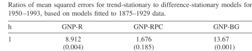
Table 2
Ratios of mean squared errors for trend-stationary to difference-stationary models for h-years-ahead forecasts, 1950 –1993, based on models fitted to 1875–1929 data.
h GNP-R GNP-RPC GNP-BG GNP-BGPC
ahead forecasts, we report in that table the portion of times that the DS forecasts outperform the TS forecasts by more than was found for the actual data sets (i.e. the proportion of times that the simulated ratio of mean squared errors exceeded the actual entry).
These are then p-values of a test of the TS specification. While it is possible to get these large values for the ratio, MSE(TS)/MSE(DS), with a true TS series it is unlikely. How unlikely? We find from Table 2 that TS can be rejected at very low significance levels for the nonper capita series. For the per capita series, the p-values are 0.185 for the Romer data and 0.154 for the Balke-Gordon data. The results thus show that if the true model is TS, then the ratio (MSE TS/MSE DS) for the simulated series will exceed the actual value only 0.4% of the time for GNP-R, 18.5% of the time for GNP-RPC, 0.1% of the time for GNP-BC and 15.4% of the time for GNP-BGPC. Given that the competitor is just a simple random walk, this represents moderately strong evidence against TS. The forecasting performance of the TS models remains surprisingly poor in a TS world, when allowing for sampling error in the parameter estimates.
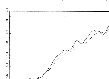
Further insight can be obtained through a more detailed examination of the one-year-ahead forecasts. Figs. 3 and 4 show logarithms of RGNP together with one-year-one-year-ahead forecasts generated from DS and TS models fitted to the Balke-Gordon data, 1875–1929. (The pictures for models fitted to the Romer data are similar). Fig. 3, for the nonper capita series clearly illustrates the difficulty of tying forecasts to a fixed trend. The forecasts from the TS models are consistently too high, particularly in the later years. As shown in Table 2, and illustrated in Fig. 4, forecasts of per-capita GNP from a TS model are somewhat less poor. Now, forecasts from the TS model are too low for much of the period. It is certainly
clear that the one-year-ahead forecast errors are not zero-mean white noise, as would be the case if the same TS model held in 1875–1929 and 1950 –1993.
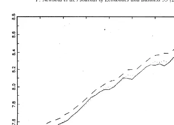
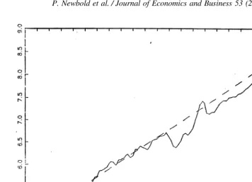
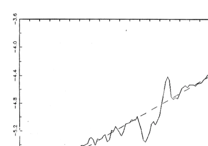
The source of the results in Table 2 can also be seen through graphs of the complete series. Figs. 5 and 6 show the two Balke-Gordon series. We have drawn on these graphs the trend lines obtained from fitting a TS model to the 1875–1929 data, and extrapolated those lines. Substantial deviations from the extrapolated trend lines in 1950 –1993 are apparent, partic-ularly for the nonper capita series.
Further examination of the one-year-ahead forecast errors is useful. For the forecast errors generated from DS models, we fitted processes of the form (3). In fact, (p,q) 5 (0,0) was selected by SBC in all cases. Table 3 shows t-ratios associated with the estimated intercept and slope parameters. Although the slope parameter estimates are moderately far from zero for the nonper capita series, there is not very strong evidence against the contention that these forecast errors are zero-mean white noise—that is, that the difference-stationary model fitted to 1875–1929 data has generated optimal forecasts in 1950 –1993.
The TS forecasts are based on first order autoregressions. If, in fact, the 1950 –1993 data are generated by a random walk, it can be shown that the one-year-ahead forecast errorset
should then follow an ARIMA (0,1,1) process
Det5b 1~12uL!et (4)
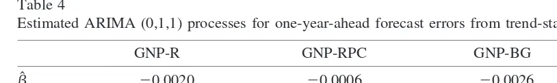
Table 4 shows parameter estimates from fitting this model to the forecast errors. Although the moving average parameter estimates are large, corresponding to the large autoregressive
parameter estimates used to generate the forecasts, they are still far from one. Moreover, the residual autocorrelations from the fitted models (4) do not suggest serious misspecification. In fact, fitting models of the form (1), with et in place of yt, to the forecast errors, the ARIMA(0,1,1) model was selected by SBC for both nonper capita series. This model was a close second choice for the two per capita series. However, the first choice in both cases was an ARIMA(1,1,1) model, with estimated moving average parameter one. This should not be taken as strong evidence of overdifferencing, as maximum likelihood estimation is very likely to produce such an outcome in sample sizes as small as this.
Our analysis of forecasts of the years 1950 –1993, generated by models fitted to the years 1875–1929 suggests that, even discounting the experience of the intervening years, station-arity around a single trend over the whole period 1875–1993 is implausible. Indeed there is little evidence against a random walk in the post-World War II years. As Diebold and Senhadji (1996) suggest, distinction between TS and DS processes can be important for forecasting purposes. We have seen that tying forecasts to an inappropriate fixed trend can generate seriously suboptimal outcomes.
5. Conclusions
Although every difference-stationary model is arbitrarily close to some trend-stationary model, when data are limited, the models of these types achieved in practice can be quite
distinct. It may then be important to distinguish between them, or indeed to conclude that neither is adequate. This distinction may be important for forecasting and modeling purposes. Our own analysis of RGNP over the period 1875–1993 suggests that neither simple trend-stationary nor difference-trend-stationary specifications are adequate. The aberrant behavior of the time series over the period 1930 –1949 is undoubtedly a strong factor in reaching this conclusion. However, even when we discount the experience of these years we find very strong evidence against a common fixed trend-stationary representation in the periods 1875–1929 and 1950 –1993. Indeed, technology shocks are for the most part permanent and most certainly not smooth. Interchangeable parts, the division of labor, the assembly line, and other older innovations still affect us positively today. Trend stationarity would seem to be incompatible with such a view. Faith in the hypothesis of trend-stationarity in RGNP over the period 1875–1993 would imply a belief that, at the beginning of time, God stretched out Her hand and drew a (straight) line in the sky, ordaining that henceforth (or at least from 1875) RGNP (measured in logarithms) would not wander arbitrarily far from that path. This paper offers a new diagnostic testing procedure that practitioners can employ when faced with conflicting results concerning TS vs. DS series.
Fig. 6. GNP-BGPC: Fitted (1875–1929) and extrapolated (1930 –1993) trend.
Table 3
t-ratios for estimated linear trend for one-year-ahead forecast errors from difference-stationary models
GNP-R GNP-RPC GNP-BG GNP-BGPC
t(aˆ ) 0.60 0.72 0.68 0.80
We do not find strong evidence against difference-stationarity in the post-World War II years, while accepting that relatively little data are available from which to uncover such evidence. The results of this paper suggest that the application of unit root tests performed over long sample periods should be done carefully with a keen eye for the type of economic shocks which impinge on the series over the full sample. In these circumstances, if a choice between difference-stationarity and trend-stationarity must be made, we prefer the former, as it implies less stringent assumptions.19For example, forecasts will not be tied to a possibly inappropriate trend line. Moreover, the spurious regression phenomenon of Granger and Newbold (1974) and Phillips (1986) would then be avoided with the DS assumption. Finally, Clements and Hendry (1999) have shown that in a world of structural breaks, using a DS model (even though it may be false) will result in lower costs in terms of forecasting accuracy since this model will adapt more rapidly to structural change than a TS model, which fixes one to a given trend.
On a more general note, we have serious doubts about the application of standard unit root tests to long annual macroeconomic time series. The hypotheses compared - trend-station-arity and difference-stationtrend-station-arity are far from exhaustive, and indeed both are a priori implausible. Moreover, it is far from clear that the position can be rectified by the procedures currently available for incorporating a very small number of structural breaks or outliers. Practical model building seeks simple parametric structures that adequately characterize a given data set. No such model is “true,” and it is difficult to believe that any could be adequate to describe the evolution of macroeconomic activity over a period of more than a hundred years. In that case, unit root tests may amount to little more than the comparison of irrelevant alternatives.
Notes
1. The use of the term Dickey-Fuller test encompasses the augmented version as well. 2. Ben-David and Papell (1995) employ modifications of the Dickey-Fuller type tests which account for structural change and examine real GDP for 16 countries. They found that most of the OECD countries analyzed exhibited trend breaks over the past 125 years. Cheung and Chinn (1996) examine the time series properties of GNP for 126 countries.
3. To be specific, the rejection of a null hypothesis amounts to the rejection of a specific parameterization, and not necessarily of TS or DS processes.
Table 4
Estimated ARIMA (0,1,1) processes for one-year-ahead forecast errors from trend-stationary models
4. Christiano and Eichenbaum (1990), Stock (1991), Rudebusch (1992, 1993), and DeJong, Nankervis, Savin, and Whiteman (1992) showed that the Dickey-Fuller test has low power to differentiate between trend-stationarity and difference-stationarity properties of real GNP. Elliot, Rothenberg, and Stock (1996) indicate that conditional volatility tends to reduce the power of unit root tests.
5. It is well documented that postwar US inflation has a large moving average component that creates large size distortions in the Dickey-Fuller tests, see Crowder and Hoffman (1996). 6. Said and Dickey (1984) and Schwert (1987) suggest using high order autoregressive
polynomials to approximate the MA component. The standard Dickey-Fuller test augmented with lagged changes is commonly referred to as the Augmented Dickey-Fuller test. In this paper the term Dickey-Dickey-Fuller will encompass both the standard and augmented versions. When the augmented version is used, the lag length employed will be specified.
7. Perron’s model implies that there was one permanent shock (a negative one) to output during the years 1909 –1970, and that all other shocks were transitory. In Perron (1989) the date of the break was assumed known. Banerjee, Lumsdaine and Stock (1992), Christiano (1992), and Zivot and Andrews (1992) argue that the date of the break should be treated as unknown a priori.
8. A test has size distortions when it rejects a true null more often than the nominal significance level,a. Type I Error: a5 Pr(rejecting H0uH0 is true).
9. The first differencing of an I(0) process should induce a moving average unit-root process. When estimating an ARIMA(2,1,1) model for postwar quarterly GNP data, Campbell and Mankiw (1987) found a moving average coefficient of20.455, while Cheung and Chinn (1997) estimated a value of 20.442. Cheung and Chinn (1997) estimate an ARIMA(2,1,1) model for annual data over the period 1869 –1986 and found a moving average coefficient of 1.0258, suggesting trend-stationary behavior for the longer span of data.
10. We took 1950 as a starting point to allow for a postwar recovery period where economic activity may have been generated by a different regime.
11. The importance of having a long time span of data in the study of persistence in real GNP has been argued in Shiller and Perron (1985) and Perron (1989).
12. Applying the structural break test of Banerjee, Lumsdaine and Stock (1992), Cheung and Chinn (1997) examined real GNP over the period 1869 –1986, and found mixed evidence for two structural breaks in trend in 1924 and 1942.
13. The models are:
15. Type II Error: b 5 Pr(not rejecting H0uH1 is true). Power 5 (1 2 b). The usual approach (called the Neyman-Pearson approach) is to fix the significance level,a, at a certain level, and minimize b. That is, choose the test-statistic that has the most power (i.e. maximize (1 2b).
16. Minor limitations include the fact that it is not clear whether this procedure accounts for model uncertainty. More importantly, evidence of instability over time in the t-statistics might be expected in the presence of macroeconomic transitional dynam-ics. Thus, one might argue that the finding of instability in the Dickey-Fuller t-statistics from the 1930s on, is not prima facie evidence of a trend break or outliers or of a unit root.
17. Diebold and Senhadji show that forecast accuracy tests based on the trough of the Great Depression strongly favor the trend stationary model, suggesting that deviation from the trend during this period is indeed stationary. This is quite possible. However, Leybourne, Mills and Newbold (1998) have shown that, if the true generating process is DS with an early (but not late) break, spurious rejections of the null of DS by Dickey-Fuller tests will frequently occur.
18. Diebold and Senhadji prefer a second order autoregressive TS model for the whole period 1875–1993. Fitting this model to the 1875–1929 data to generate forecasts for 1950 –1993 yielded results that differed little from those of Table 2, and in fact the estimated second order autoregressive parameters were all close to zero.
19. For example, one can think of an I(1), DS series as a slowly evolving trend over time. If one restricts the trend to be fixed, so it is not able to evolve at all, you have a TS series. In this sense trend-stationarity is more restrictive than difference-stationarity.
Acknowledgments
The authors would like to thank Chris Murray and Charles Nelson for helpful comments on an earlier draft of this paper.
References
Agiakloglou, Christos & Paul Newbold. (1992). Empirical evidence on Dickey-Fuller-type tests,Journal of Time Series Analysis, 13, 471– 83.
Agiakloglou, Christos & Paul Newbold. (1996). The balance between size and power in Dickey-Fuller tests with data-dependent rules for the choice of truncation lagEconomics Letters, 52, 229 –34.
Balke, Nathan S., & Thomas B. Fomby, “Shifting Trends, Segmented Trends, and Infrequent Permanent Shocks,” Journal of Monetary Economics, 28(1991), 61– 85.
Balke, Nathan S., & Gordon, Robert J., “The Estimation of Pre-war Gross National Product: Methodology and New Evidence,”Journal of Political Economy, 97(February, 1989), 38 –92.
Banerjee, A., Lumsdaine, R., & James H. Stock, “Recursive and Sequential Tests of the Unit Root and Trend Break Hypotheses: Theory and International Evidence,” Journal of Business and Economic Statistics, 10(1992), 271–287.
Campbell, John Y., & Gregory N. Mankiw, “Are output fluctuations transitory?”Quarterly Journal of Econom-ics, 102(November 1987), 857– 80.
Cheung, Yin-Wong W., & Menzie D. Chinn, “Further investigation of the uncertain unit root in GNP,”Journal of Business and Economic Statistics, 15(January 1997), 68 –73.
Cheung, Yin-Wong W., & Menzie D. Chinn, “Deterministic, Stochastic, and Segmented Trends: A Cross Country Analysis,”Oxford Economics Papers, 48(1996), 134 –162.
Christiano, Lawrence J., & Martin Eichenbaum, “Unit roots in real GNP: Do we know and do we care?” Carnegie-Rochester Conference Series on Public Policy, 32(Spring 1990), 7– 61.
Christiano, Lawrence J., “Searching For a Break in GNP,”Journal of Business and Economic Statistics, 10(1992), 237–250.
Clements, Michael P., & David F. Hendry, Forecasting Non-Stationary Time Series(Cambridge, MIT Press 1999).
Cochrane, John H., “A Critique of the Application of Unit Root Tests,”Journal of Economic Dynamics and Control, 15(1991), 275–284.
Crowder, William J., & Dennis L. Hoffman, “The Long Run Relationship between Nominal Interest Rates and Inflation: The Fisher Equation Revisited,” Journal of Money, Credit and Banking, 28(February 1996), 102–118.
Cryer, J. D., & Ledolter, J., “Small sample properties of the maximum likelihood estimator in the first order moving average model,”Biometrika, 68(1981), 691– 4.
Davis, Richard A., & W. T. M. Dunsmuir, “Maximum likelihood estimation for MA(1) processes with a root on or near the unit circle,”Econometric Theory, 12(March 1996), 1–29.
DeJong, David N., Nankervis, J. C., Savin, N. E., & C. H. Whiteman, “Integration Versus Trend Stationarity in Time Series,”Econometrica, 60(1992), 423– 433.
Diebold, Francis X., & Abdelhak S. Senhadji, “The uncertain root in real GNP: Comment”American Economic Review, 86(December 1996), 1291– 8.
Dickey, David A., & Wayne A. Fuller, “Distribution of the estimators for autoregressive time series with a unit root,”Journal of the American Statistical Association, 74(June 1979), 427–31.
Elliot, Graham, Rothenberg, Thomas J., & James H. Stock, “Efficient Tests for An Autoregressive Unit Root,” Econometrica, 64(1996), 813– 836.
Evans, G. W., “Output and Unemployment Dynamics in the US,”Journal of Applied Econometrics, 4(1989), 213–237.
Faust, Jan, “Near observational equivalence and theoretical problems with unit root tests,”Econometric Theory, 12(October 1996), 724 –31.
Franses, Phillip H., & Niels Haldrup, “The effects of additive outliers on tests for unit roots and cointegration,” Journal of Business and Economic Statistics,(October 1994), 471– 8.
Granger, Clive W. J., & Paul Newbold, “Spurious regressions in econometrics,”Journal of Econometrics, 2(July 1974), 111–20.
Hannan, E. J., “The Estimation of the Order of an ARMA Process,”Annals of Statistics, 10(1982), 1071– 81. Kilian, Lutz, & Lee E. Ohanian, “Is There a Trend Break in US GNP? A Macroeconomic Perspective,”Federal
Reserve Bank of Minneapolis Working Staff Report, 244(January 1998).
Leybourne, Stephen J., & B. P. M. McCabe, “A consistent test for a unit root,”Journal of Business and Economic Statistics, 12(April 1994), 157– 66.
Leybourne, Stephen J., & B. P. M. McCabe, (1996). “Modified stationarity tests with data-dependent model selection rules,” Discussion paper, Department of Economics, University of Nottingham.
Leybourne, Stephen J., Mills, Terence C., & Paul Newbold, “Spurious rejections by Dickey-Fuller tests in the presence of a break under the null,”Journal of Econometrics, 87(November 1998), 191–203.
Nelson, Charles R., & Charles I. Plosser, “Trends and Random Walks in Macroeconomic Times Series,”Journal of Monetary Economics, 10(1982), 139 –162.
Ng, Serena, & Pierre Perron, “Unit root tests in ARMA models with data-dependent methods for the selection of the truncation lag,”Journal of the American Statistical Association, 90(March 1995), 268 –281.
Perron, Pierre, “The great cash, the oil price shock, and the unit root hypothesis,”Econometrica, 57(November 1989), 1361– 401.
Perron, Pierre, & Peter C. B. Phillips, “Does GNP Have a Unit Root?”Economic Letters, 23(1987), 139 –145. Phillips, Peter C. B., “Understanding spurious regressions in econometrics,”Journal of Econometrics,
33(De-cember 1986), 311– 40.
Romer, Christina D., “The Pre-war Business Cycle Reconsidered: New Evidence of Gross National Product, 1869 –1908,”Journal of Political Economy, 97(February, 1989), 1–37.
Rudebusch, Glen D., “Trends and Random Walks in Macroeconomic Time Series: A Re-Examination,” Inter-national Economic Review, 33(1992), 661– 680.
Rudebusch, Glen D., “The Uncertain Unit Root in Real GNP,”Economic Letters, 83(1993), 264 –272. Said, S. E., & David A. Dickey, “Testing For Unit Roots in Auto-Regressive Moving Average Models of
Unknown Order,”Biometrika,(1984), 599 – 608.
Schwert, G. W., (1987). “Effects of Model Specification on Tests for Unit Roots in Macroeconomic Data,” Journal of Monetary Economics, 20,73–103.
Schwert, G. William, “Tests for unit roots: a Monte Carlo investigation,”Journal of Business and Economic Statistics, 7(1989), 147–59.
Shephard, N. G., & Andrew C. Harvey, “On the probability of estimating a deterministic component in the local level model,”Journal of Time Series Analysis, 11(1990), 339 – 47.
Shiller, Robert J., & Pierre Perron, “Testing the Random Walk Hypothesis: Power Versus Frequency of Observation,”Economic Letters, 18(1985), 381–386.
Stock, James H., & Mark W. Watson, “Does GNP Have A Unit Root?”Economic Letters, 22(1986), 147–151. Stock, James H., “Unit Roots, Structural Breaks, and Trends,” in Z. Griliches and M. D. Intriligator (eds.)
Handbook of Econometrics,(New York, North-Holland) (1994, Chapter 46).
Tsay, R. S., “Model checking via parametric bootstraps in time series analysis,”Applied Statistics, 41(1992), 1–15.