Conjunctive surface–subsurface modeling of
overland flow
Vivekanand Singh* & S. Murty Bhallamudi
Department of Civil Engineering, Indian Institute of Technology, Kanpur, India(Received 10 June 1996; revised 10 January 1997; accepted 28 May 1997)
In this paper, details of a conjunctive surface–subsurface numerical model for the simulation of overland flow are presented. In this model, the complete one-dimensional Saint-Venant equations for the surface flow are solved by a simple, explicit, essentially non-oscillating (ENO) scheme. The two-dimensional Richards equation in the mixed form for the subsurface flow is solved using an efficient strongly implicit finite-difference scheme. The explicit scheme for the surface flow component results in a simple method for connecting the surface and subsurface components. The model is verified using the experimental data and previous numerical results available in the literature. The proposed model is used to study the two-dimensionality effects due to non-homogeneous subsurface characteristics. Applicability of the model to handle complex subsurface conditions is demonstrated. q1998 Elsevier Science Limited. All rights reserved
Key words: Overland flow, Saint-Venant equations, Richards equation, Conjunctive model.
1 INTRODUCTION
Overland flow is a dynamic part of a watershed response to the rainfall and has many engineering applications, such as (i) water budgeting, (ii) flood prediction, (iii) soil erosion studies, (iv) investigations into infiltration process, (v) trans-port of pollutant to streams, and (vi) design of runways and parking lots. Mathematical modeling of overland flow involves the solution of the governing equations for both the surface flow and the groundwater flow with seepage at the ground surface acting as the connecting link. The level of model sophistication depends on the assumptions made for simplifying the governing equations before they are solved. Many models consider only the surface flow system along with an empirical treatment of the infiltration term. On the other hand, some models consider both the surface and the subsurface flow systems, but use either a diffusion wave or a kinematic wave approximation for modeling overland flow.
Akan 3,4, Sunada and Hong 30, De Lima and Van der Molen 13, and Govindaraju et al. 17 developed overland flow models based on the kinematic wave approximation.
It should be noted here that the kinematic wave approxima-tion fails for highly subcritical flows on flat slopes and when the downstream boundary condition is an important factor
25
. Diffusion wave models are applicable over a wider range of flow conditions and, therefore, may be used for such cases. Hromadka et al.21developed a two-dimensional dif-fusion wave model assuming a constant effective rainfall intensity. Govindaraju et al. 15 derived an approximate analytical solution to overland flow under a specified net lateral inflow using the diffusion wave approximation. They also provide the complete numerical solutions for the diffusion wave equation. Todini and Venutelli 32 also developed a similar two-dimensional diffusion wave model in which the governing equations were solved by the finite-difference as well as the finite-element methods.
Vieira 33 conducted a comprehensive study of various approximations usually applied to the Saint-Venant tions. It was suggested that the complete Saint-Venant equa-tions should be used in cases where the kinematic wave number is less than 5. Although, the overland flow models based on the complete Saint-Venant equations are compu-tationally very intensive, they are more versatile and can also act as standards of comparison for simplified models. Among the earliest full dynamic models are those developed q1998 Elsevier Science Ltd Printed in Great Britain. All rights reserved 0309-1708/98/$19.00 + 0.00
PII: S 0 3 0 9 - 1 7 0 8 ( 9 7 ) 0 0 0 2 0 - 1
by Woolhiser and Liggett34and by Lin et al.24. Chow and Ben-Zvi12and Kawahara and Yokoyama22developed two-dimensional overland flow models for impervious surfaces based on the Lax–Wendroff method23and a finite-element method, respectively. Zhang and Cundy37developed a two-dimensional overland flow model for a temporally constant, but spatially varying infiltration. MacCormack finite-differ-ence method was used to obtain the numerical solution. Tayfur et al.31also developed a two-dimensional overland flow model based on an implicit method 8for solving the governing equations and applied the model to experimental hill slopes. It was reported that consideration of microtopo-graphy in fine detail could result in numerical instability and convergence problems.
All the overland flow models discussed so far describe the infiltration process in an empirical way. Smith and Woolhiser 29 were probably the first to develop a con-junctive model for overland flow. They solved the one-dimensional Richards equation for unsaturated flow in the subsurface together with the one-dimensional kinematic wave equation for the surface flow. The Richards equation was solved by an implicit Crank–Nicolson finite-difference formulation. Akan and Yen5developed a sophisticated con-junctive model in which they solved the complete Saint-Venant equations and the two-dimensional Richards equation. The Saint-Venant equations were solved by the four-point implicit method, while Richards equation was solved by the SLOR technique. In the very versatile, com-plete catchment model, SHE2, the overland flow component is simulated using the diffusion wave approximation. The subsurface flow in the unsaturated zone is represented by the one-dimensional Richards equation. The surface flow equa-tions are solved by the explicit procedure developed by Preissmann and Zaoui 28, while the Richards equation is solved by the implicit finite-difference scheme. Govindaraju and Kavvas 16, in a detailed study of hillslope hydrology through a stream flow—overland flow—subsurface flow model, used the diffusion wave approximation for the sur-face flow component. The sursur-face flow equation was solved by the centred implicit scheme, while the two-dimensional Richards equation was solved by the SLOR technique.
In this paper, an alternative conjunctive numerical model is presented for simulating the overland flow. The numerical model is based on a conjunctive solution of the complete Saint-Venant equations for the surface flow and the two-dimensional Richards equation. Presently available full dynamic models for the overland flow employ classical second-order accurate finite-difference methods for solving the Saint-Venant equations. These methods often result in high frequency oscillations when there are sharp changes in the flow parameters and require ad hoc procedures for obtaining smooth solutions 6. In this study, a simple to implement high-resolution essentially non-oscillating (ENO) scheme27is applied to solve the surface flow com-ponent in the conjunctive model. The explicit ENO scheme also results in a simple method for connecting the surface and subsurface flow components. Presently available
conjunctive models for the overland flow use Richards equation in pressure-head form, which may result in signi-ficant mass balance error for complex subsoil conditions. Many studies 7,19,9 have shown that the ‘mixed form’ of the Richards equation results in better numerical behaviour than the other forms. Therefore, in this study, the two-dimensional Richards equation in the mixed form is used for simulating the subsurface component. This equation is solved by a recently developed strongly implicit procedure
20. This is computationally more efficient than the SLOR
technique adopted in the currently available conjunctive models. The proposed numerical model is verified using the experimental data available in the literature29. Robust-ness of the numerical model is demonstrated by considering a test case in which a clay lens is present in the subsurface. One of the objectives of developing a sophisticated model is that it can act as a standard of comparison for simplified models. Therefore, the proposed numerical model is used to study the errors that may result in the prediction of the out-flow hydrograph if a one-dimensional simulation of the sub-surface flow is used.
2 GOVERNING EQUATIONS
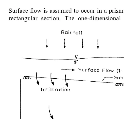
Mathematical modeling of overland flow involves the solu-tion of the governing equasolu-tions for both the surface flow and the groundwater flow with seepage at the ground surface acting as the connecting link. In the present study (Fig. 1), the surface runoff is represented by the one-dimensional flow equations in the x-direction, while the groundwater flow is represented by the two-dimensional Richards equa-tion in the x and z direcequa-tions.
2.1 Surface flow equations
Surface flow is assumed to occur in a prismatic channel of rectangular section. The one-dimensional shallow water
flow equations in conservation form for such a case are ¼volumetric rate of rainfall per unit surface area (m/s); I¼ volumetric rate of infiltration per unit area (m/s); S0 ¼
bottom slope in the direction of flow; Sf ¼friction slope;
x¼distance along the flow direction (m); and t¼time (s). The assumptions and the derivation of the above equations have been reported earlier36,1,11and are not repeated here. The friction slope, Sf is computed using the Darcy–
Weisbach formula taking into account the effect of rainfall on frictional resistance.
Sf¼fd q2
8gh3 (3)
in which, fd¼frictional resistance coefficient. Evaluation
of fddepends on the instantaneous state of flow. The flow is
laminar in all the studies reported here and, therefore, fdis
given by the following equation5. fd¼
CL
Re (4)
where Re ¼ Reynolds number ¼ q/v (v ¼ kinematic viscosity of water), and CL is a constant which depends
on the rainfall intensity.
2.2 Subsurface flow equations
In the present study, subsurface flow is modeled as two-dimensional motion of a single-phase incompressible fluid in an incompressible porous medium. The two-dimensional, transient flow equation in an isotropic porous medium is derived by applying the principle of conservation of mass. This equation without sources and sinks within the flow domain can be written as
]v
where,v¼volumetric moisture content; Vxand Vz¼darcy flow velocity in the x and z direction, respectively, and x and z are distances along the two coordinate directions; z is taken positive downwards. It is assumed that the Darcy’s law is applicable for evaluating the velocity components. hydraulic conductivity (m/s) which depends on the pressure head, w. Substitution of eqn (6) in eqn (5) yields the Richards equation14:
]v
eqn (7) is said to be in ‘mixed form’ since it includes both the dependent variables v and w. Hydraulic relationships between the pressure head,w, and the hydraulic conductiv-ity, K (w–K relationship), and between the moisture con-tent, v, and the pressure head w (w–v relationship), are needed while solving eqns (5) and (6) in the unsaturated zone. In general, w–K and w–v relationships are not unique and soils exhibit different behaviour during wetting and drying phases. This hysteresis in soil charac-teristics is not considered for the cases studied in the present work. However, the hysteresis can be included by employing differentw–K andw–vrelationships for wet-ting and drying processes. Although semi-analytical equations are available for describing w–K andw–v rela-tionships, the soil characteristics derived from the experi-mental and field data are employed wherever available. These relationships are specific to the case studied and are described later.
3 NUMERICAL SOLUTION 3.1 Surface flow
Surface flow equations constitute a set of nonlinear hyper-bolic partial differential equations. A recently developed high-resolution essentially non-oscillating (ENO) scheme for solving the shallow water flow equations27is employed in the present study to solve the surface flow equations. The scheme, proposed by Nujic 27, is modified suitably to account for the non-zero source term in the continuity equa-tion. This scheme, unlike many other classical second-order accurate schemes such as the MacCormack method, is non-oscillatory even when sharp gradients in the flow variables are present. The main advantages of this scheme are its simplicity, ease of implementation and ease of extension to a two-dimensional case. It is also very attractive for the present application because it is possible to account for the variable bottom topography in a convenient and accurate way. It is an explicit, two-step predictor–corrector scheme which results in second-order accuracy in both space and time. Only a brief description of the method as applied in the present study is outlined here.
3.1.1 Predictor part
explicit determination of Ui*is written as where Fiþ1/2n represents the numerical flux through the cell
face between nodes iþ1 and i.Dx is the grid spacing and
Dt is the computational time step. All the terms on the
right-hand side of eqn (8) are evaluated at the known time level n and, therefore, Ui*can be computed explicitly. The numerical flux Fiþ1/2 is computed using the following
formula.
computed using the information from the right side of the cell face and FL ¼ f(UL) ¼the flux computed using the
information from the left side of the cell face. ULand UR
are obtained using a MUSCL (monotone upwind scheme for conservation laws) approach.
UL¼Uiþ
There are several ways of determining dUi and dUiþ1
using different slope limiter procedures 6,35. The ‘minmod’ limiter is followed in the present study. Accord-ing to this,
dUi¼minmod(Uiþ1¹Ui, Ui¹Ui¹1) (12)
where the minmod function is defined as
minmod(a,b)¼
The positive coefficient a is determined using the maxi-mum value (for all the grid points) of the largest eigen value of the Jacobian of the system of equations. This is given as
where, N is the total number of grid points. The vector equation (eqn (8)) gives the predicted values of h and q at the unknown time level at any node i.
3.1.2 Corrector part
The vector U at the unknown time level nþ1 and at node i, i.e. Uinþ1 is computed using the predicted values and the values at the time level n.
Uinþ1¼0:5 U
Following the recommendations of Alcrudo et al.6, UR*and
UL*are determined from Ui*þ1and Ui*using the samedUiþ1 anddUias determined in the predictor step. This procedure results in better numerical stability.
In eqn (15), only the source term in the momentum equa-tion (the second component of the vector equaequa-tion) is eval-uated using the predicted values of h and q. However, the source term in the continuity equation i.e. (R¹I)iis eval-uated using the values at the known time level instead of the predicted values. Strictly speaking, this procedure decou-ples the subsurface flow computations and the surface flow computations during the computational time step Dt. However, the response of the subsurface flow to the varia-tion in surface flow depth is much slower than the response of surface flow to changes in the rate of infiltration5. There-fore, the above decoupling does not affect the results sig-nificantly. In fact, numerical experimentation showed that determination of the infiltration rate, I, during the corrector step by using the predicted flow depth did not alter the results. On the other hand, the decoupling procedure resulted in significant savings of the computational time, since the subsurface flow is computed only once during a time step.
3.2 Initial and boundary conditions
Values of the flow depth, the discharge and the infiltration rate are specified at all the nodes at time t¼0 as the initial conditions. The initial infiltration rate is equal to the rainfall rate. Although the initial flow depth and the discharge are equal to zero (overland flow on an initially dry surface), a very thin water film of depth hiniand corresponding uniform
flow discharge, qiniare assumed to exist at time t¼0. This
assumption is made to overcome the numerical singularity in a simple way. However, it should be noted that the out-flow hydrograph may be sensitive to the hini value and,
therefore, it should be chosen as small as possible. The explicit finite-difference scheme described earlier can be used to determine h and q at the unknown time level only at the nodes i ¼2 to N¹1. The values of the variables at the upstream and the downstream ends of the domain are determined using the appropriate boundary con-ditions. The discharge at the upstream end is equal to zero. However, the discharge at the upstream end is specified as qini to be consistent with the initial conditions. The flow
3.3 Stability condition
The high-resolution Lax–Friedrichs scheme adopted in the present study is an explicit scheme. Therefore, the computa-tional time step,Dt, is chosen using the CFL condition.
Cn¼
in which Cn¼Courant number.Dt is chosen dynamically
in the numerical model such that eqn (17) is satisfied at all the nodes i¼1,2…N.
3.4 Subsurface flow
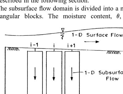
In order to determine the infiltration rate I in the continuity equation for the surface flow, the subsurface flow equations have to be solved along with an appropriate boundary con-dition at the ground surface. In the present study, a recently developed strongly implicit finite-difference scheme20for the mixed based formulation of the Richards equation is used to simulate the unsaturated subsurface flow conditions. This scheme ensures mass balance in its solution regardless of time step size and nodal spacings, and has no limitations when applied to field problems. It is also easy to incorporate different types of boundary conditions in this scheme. In the present study, two different models 1DS2DSS and 1DS1DSS are developed for simulating the overland flow. In the model 1DS2DSS (one-dimensional surface flow with two-dimensional subsurface flow), the infiltration rate, I, is determined by solving the two-dimensional Richards equa-tion. In the model 1DS1DSS (one-dimensional surface flow with one-dimensional subsurface flow), the subsurface flow is assumed to occur only in the vertical direction. Fig. 2 shows the definition sketch for the model 1DS1DSS. In this model, the infiltration rate at any distance x is deter-mined using the one-dimensional Richards equation with the surface flow depth at that point as the top boundary condition. Model 1DS1DSS results in significant savings of CPU time. Numerical solution of the Richards equation is described in the following section.
The subsurface flow domain is divided into a number of rectangular blocks. The moisture content, v, and the
pressure head, w, are specified at the center of the block (the node), while the velocities are specified at the inter-block faces. The subscript i refers to the inter-block number in the x direction and the subscript j refers to the block number in the z direction. The superscripts n and nþ1 refer to the known and the unknown time levels, respectively. The finite-difference form of the eqn (5) is
vni,þj 1¹v
where the bar is used to denote the time-averaged value of the velocity.Dx andDz are the nodal spacings in the x and z directions, respectively. The time-averaged velocities are determined by
¯
V¼wVnþ1þ(1¹w)Vn (19)
in which, w ¼time weighting factor. The velocity at any interblock face is determined using the pressure heads at the neighbouring cell centers. For example;
Vi,jþ1=2¼ ¹Ki,jþ1=2[(wi,jþ1¹wi,j)¹Dz]=Dz (20) in which, Ki,jþ1/2is the unsaturated hydraulic conductivity
evaluated at the interblock faces between the nodes (i,jþ1) and (i,j). Substitution of eqns (19) and (20) in eqn (18) yields
The unsaturated hydraulic conductivity at an interblock face is estimated using the pressure heads at the neighbour-ing cell centers. Cooley10, Haverkamp and Vauclin 18and Narasimhan and Witherspoon 26 have suggested various ways for this purpose. Haverkamp and Vauclin 18 state that the geometric mean is the best choice for estimating the interblock conductivities. However, Hong et al. 20 reported (also experienced during the development of the present model) that the iterative solution of eqn (21) fails to converge if the above procedure is adopted for estimating the K value. This is especially true for infiltration into initially very dry soils. The geometric mean is strongly weighted towards the lower value and, therefore, water cannot drain easily if the soil is initially dry. This results in a non-physical build up of pressure. In this study, the interblock hydraulic conductivity is estimated by the
weighted arithmetic mean. For example,
Ki,jþ1=2¼gK(wi,j)þ(1¹g)K(wi,jþ1) (22)
in which,gis the weight coefficient. Hong et al.20suggest a value of 0.5 forg. Eqn (21) is written for all the blocks in the flow domain and this results in a set of simultaneous algebraic equations in the unknownswi,jnþ1. These simulta-neous equations are highly non-linear sincevnþ1and Knþ1 are non-linear functions ofwnþ1. In the present study, they are solved by using the Newton–Raphson technique.
3.5 Boundary conditions
3.5.1 Flux-type boundary conditions
In the adopted scheme, the grid is arranged in such a manner that the boundaries of the flow domain coincide with an interblock. Therefore, flux or velocity-type boundary con-ditions can be incorporated in a natural way in eqn (18).
3.5.2 Pressure head-type boundary conditions
The imposed pressure head at the boundary is used along with the values of pressure head at the neighbouring interior points to determine the flux at the boundary. Second-order one-sided finite-difference analog is used for this purpose
3.6 Surface and subsurface flow interaction
Surface and subsurface flow components are interrelated by a common pressure head and the infiltration at the ground surface. The top boundary condition for the subsurface flow is determined by the surface flow depth. In turn, the infiltra-tion term in the surface flow equainfiltra-tion is controlled by the subsurface flow conditions. The following procedure is adopted for simulating the interaction between the surface and the subsurface flow components.
1. Subsurface flow solution at time level n is used to determine the infiltration rate at the ground surface. 2. Surface flow equations are now solved using the
infil-tration rate from step 1 to determine q and h at the unknown time level n þ1.
3. The surface flow depth at the time level nþ1 is used as the top boundary condition and the subsurface flow equations are solved. This gives thevandw distribu-tion in the subsurface at time level nþ1.
4. Steps 1–3 are repeated up to the required time level. As mentioned earlier, the above is a decoupled approach which reduces the CPU time by half without significantly affecting the accuracy of the results.
3.7 Boundary conditions
For subsurface flow resulting from rainfall infiltration, the top boundary condition changes with time. During the initial stages of the rainfall, there is no ponding and the infiltration rate is equal to the rainfall rate. The top boundary condition for such a situation is the specification of the flux equal to
the rainfall rate. As time progresses, the upper layers of the subsoil become saturated and then infiltration rate starts decreasing. Before starting the solution of the Richards equation for any time step, the flux at the top boundary is estimated by takingwb¼0. If this velocity is greater than
the rainfall rate, then the flux type of boundary condition is applied. Otherwise, a head type of boundary condition
(wb(x) ¼ h(x) water flow depth at that point) is applied.
The time to ponding comes out as a part of the solution. Specified head or specified flux conditions can be imposed at the lateral and bottom boundaries. For the physical situations considered in the present study, a no-flux boundary condition is imposed at the right and left boundaries. The w values at the bottom boundary are obtained using a simple extrapolation from the interior points. This approximation does not introduce errors because the bottom boundary is taken fairly deep and the moisture front does not reach that far for the computational times considered.
4 VERIFICATION OF THE MODEL
The model presented in the previous section is tested with the experimental data of Smith and Woolhiser29for a con-junctive surface–subsurface flow. The experiments29were conducted in a soil flume of 12.2 m length, 51 mm wide and 1.22 m deep. The slope of the channel was 0.01. The fluid used was a light oil whose viscosity v¼1.94310¹4m2/s. A rainfall simulator was used to produce a rainfall of inten-sity 250 mm/h over a duration of 15 min. The flow regime is laminar throughout and the CLvalue5in eqn (4) is taken as
92.0. The soil used was Poudre fine sand and it was placed in three layers of differing bulk densities. Thicknesses of the three layers, 1, 2 and 3, were 76.5, 229.5 and 761 mm, respectively. The hydraulic properties (vvs.wand K vs.w
curves) of the three layers were determined experimentally
29
. The relative hydraulic conductivity, Krand the effective
saturation, Seare defined as
Kr¼
in which, Ksandvsare the saturated hydraulic conductivity
and saturated moisture content,vris the residual moisture
content. The curves for Se vs. pressure head and Kr vs.
Kr
pressure potential) for the three soil layers are given in the Table 1.
The numerical model is run for a length of 15 m with 2.8 m acting as the buffer length for application of the downstream boundary condition. The finite-difference grid spacings in the x and z directions, Dx and Dz, are equal to 0.25 m and 12.7 mm, respectively, and Courant number Cn¼0.65. A very small value of 0.2 mm is taken as the
initial flow depth, hini. The numerical parameters for
the subsurface flow computations are: w ¼ 1.0, g ¼ 0.5 and e ¼ 10¹3. Although, only a high-resolution (ENO) scheme for the surface flow is presented in this paper, the surface flow equations were also solved using the classical
MacCormack scheme 11 as a double check. Both the methods gave essentially the same results for this run.
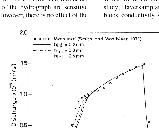
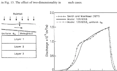
Fig. 3 shows the runoff hydrograph at the downstream end (x ¼12.25 m) for the above experiment obtained (i) experimentally 29, (ii) numerically by Akan and Yen 5, (iii) numerically by the model 1DS1DSS and (iv) numeri-cally by the model 1DS2DSS. It is clear from this figure that both the models 1DSlDSS and 1DS2DSS give almost the same results. Model 1DS2DSS shows only some marginal effect of two-dimensional subsurface flow. It can be seen that the numerical results obtained by the models 1DS1DSS and 1DS2DSS compare satisfactorily with the experimental as well as with the earlier numerical results of Akan and Yen5. The present numerical results are lagging as far as the rising limb of the hydrograph is concerned. However, they are better for the recession phase. The discrepancy between the present numerical results and the earlier numerical results of Akan and Yen5could be due to minor differences in processing the soil-moisture characteristic curves as given by Smith and Woolhiser 29. It should be noted here that the results for the outflow hydrograph are sensitive to the hydraulic properties of the subsurface soil. A 2.8% decrease in the Ks value for layer 1 and a corresponding
2.8% increase in the Ks value for layer 2 resulted in an
outflow hydrograph which matched very well with the experimental data. Fig. 4 shows the volumetric saturation profile under the ground along the depth at a distance of 5.5 m from the upstream end at different times. This figure shows the present numerical results and the previous numerical results obtained by Smith and Woolhiser29. No attempt is made to compare the numerical results with the experimental data because the data points are very few in number. It can be seen from Fig. 4 that the present and previous numerical results of Smith and Woolhiser 29 match satisfactorily at early times. However, as time pro-gresses, the wetting front in the present model moves faster than the wetting front in Smith and Woolhiser’s 29model
Table 1. Hydraulic properties of the soil
Layer Ks
Fig. 3. Verification of models 1DS1DSS and 1DS2DSS: outflow
because the computed infiltration rate is larger. This is con-sistent with the results presented in Fig. 3, where the outflow hydrograph by the present model is lagging the previous results. Fig. 4 also shows that the two-dimensional subsur-face flow effects are marginal for the particular case studied here.
Sensitivity of the numerical results to the numerical parameters hini, and the weighting coefficient,g, is studied
using the model 1DS1DSS. Fig. 5 shows the effect of ad hoc specification of the initial flow depth, hini. Initial flow depth
in these runs varied from 0.2 to 0.5 mm. The numerical results for the rising limb of the hydrograph are sensitive to the specified hinivalue. However, there is no effect of the
hini on the hydrograph beyond a certain time (11 min).
Although it appears that better results can be obtained by taking hini¼0.5 mm, this value should be chosen as small as
possible in order to faithfully represent the initial dry con-ditions. The effect of weighting coefficient,g(in the deter-mination of the interblock hydraulic conductivity), on the outflow hydrograph is shown in Fig. 6. It is obvious from Fig. 6 that the numerical results are highly sensitive to theg
value. Hong et al. 20 recommended a value of 0.5 for g, which results in equal weightage to higher and lower values of K on the two sides of the face. In an earlier study, Haverkamp and Vauclin18concluded that the inter-block conductivity should be weighted more towards the
Fig. 4. Verification of models 1DS1DSS and 1DS2DSS: volumetric saturation in subsurface.
lower value of K and, accordingly, they used the geometric mean. In the limit of grid convergence,g¼0.35 gave better results thang¼0.5 for the test case studied here. However, the above conclusion cannot be generalized because it is based on a comparison of numerical results with experimen-tal data which may have uncertainties in them. This aspect needs further study.
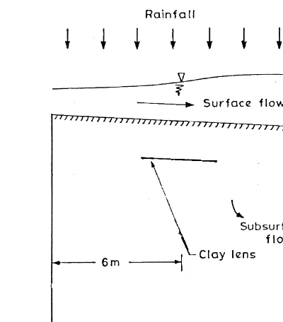
Often soil deposits are encountered in the field (Ex: Allu-vial deposits) which are more or less homogeneous except for the presence of an isolated clay lens. This clay lens acts as a barrier to the vertical movement of the wetting front in the ground, and can significantly affect overland flow. In such a case, sharp gradients may occur in the overland flow hydrograph, and models which use traditional numerical methods result in numerical oscillations. This is demon-strated by considering a case (Fig. 7) in which a clay lens of length 4 m is present at a depth of 11.4 cm from the surface. The subsoil characteristics for this run were same as those for layer 1 in the experiments by Smith and Wool-hiser29. Other input parameters, such as the rainfall rate and length of the domain, were also same. The outflow hydro-graphs for this case, obtained using (i) the model 1DS2DSS with ENO scheme, and (ii) the model 1DS2DSS with a traditional finite-difference scheme, such as the Mac-Cormack method, are compared in Fig. 8. A Courant number of 0.8 was used for the ENO scheme while a value of 0.75 was used for the MacCormack scheme. It is very clear from Fig. 8 that the numerical results obtained using the ENO scheme are superior to those obtained using the MacCormack scheme. A Courant number value as low as 0.2 was required to suppress the numerical oscillations in the MacCormack scheme. This is also the order of Courant number used by Zhang and Cundy37in some of their simu-lations. It should be noted here that low Courant number values result not only in higher computational times, but also in diffusive errors 11. Numerical results for this test case also demonstrate that the model 1DS2DSS can be
used to simulate the effect of complex subsurface conditions on an overland flow hydrograph. Immediately after the arri-val of the wetting front at the clay lens, the infiltration rate for that part of the channel which is directly above the clay lens becomes negligible, and there is a sharp rise in the outflow hydrograph. Model 1DS2DSS was able to simulate this effect.
5 SIMPLIFIED MODELING
One of the objectives of developing a sophisticated model is that it can act as a standard of comparison for simplified models. Some of the currently available conjunctive models for the overland flow2,29assume that the subsurface flow in the unsaturated zone is predominantly one-dimensional. Therefore, a one-dimensional Richards equation is used in their models. Govindaraju and Kavvas16have demonstrated how such an assumption is not valid if the groundwater table is close to the surface. Herein, the model 1DS2DSS is used to study the error in the prediction of the outflow hydrograph using a one-dimensional simulation of the subsurface flow for the case of a deep groundwater table. Three different hypothetical cases, as represented in Fig. 9, are considered for this purpose. In this figure, the soil characteristics of layers 1, 2 and 3 are same as the soil characteristics for layers 1, 2 and 3 in the experiments by Smith and Woolhiser
29. The same surface flow conditions (length¼15 m, slope ¼0.01, v¼1.943104m2/s, R¼250 mm/h, CL¼92.0) are
used in these simulation runs. The numerical simulations are performed usingDx¼0.25 m, hini¼2310
¹3
m,a¼1.0 andg¼0.5, in both models, 1DS1DSS and 1DS2DSS. In Fig. 10, the outflow hydrograph for the case shown in
Fig. 6. Effect ofgon the overland flow hydrograph.
Fig. 7. Schematic representation of case considered for studying
Fig.9(a) is compared with the outflow hydrograph for Smith and Woolhiser’s29 experiment. Both the hydrographs are obtained using the model 1DS1DSS. It can be observed from Fig. 10 that the ad hoc simplification of layered soil conditions in Smith and Woolhiser’s 29 experiment by a single layer, as given in Fig. 9(a), affects the outflow hydro-graph significantly. This is because the spatial variation in soil characteristics in the vertical direction affects the infil-tration rate. Appropriate homogenization procedures should be adopted if simple analytical solutions for infiltration
based on homogeneous soil characteristics are to be used while simulating overland flow on layered subsoil. In the absence of appropriate homogenization, model 1DS1DSS can be used to study the effect of subsoil layering on the outflow hydrograph. Application of the computationally more intensive model 1DS2DSS is not required if there is only vertical layering in the subsoil. Both models, 1DS1DSS and 1DS2DSS, gave essentially the same results (not shown here) for the case shown in Fig. 9(a). For this case of uniform rainfall rate, the whole surface length is ponded at the same time, and the wetting front moves essen-tially in the vertical direction. The two-dimensional subsur-face flow effects are only marginal and models 1DS1DSS and 1DS2DSS give similar results. Model 1DS1DSS is also run for Smith and Woolhiser’s 29experiment by assuming that the infiltration rate is uniform throughout the length, as schematically represented in Fig. 11(a). Such an assumption is valid if the surface flow depth does not have a significant effect on the infiltration rate. Fig. 11(b) compares the out-flow hydrograph from this run with the previous outout-flow hydrograph obtained using the general 1DS1DSS model. It can be clearly seen that both the hydrographs are essen-tially the same. This indicates that the infiltration rate is more or less uniform throughout the length as long as there is no spatial variability of soil characteristics in the x direction. The non-uniform surface flow depth does not have a significant effect on the infiltration rate. This assumption of uniform infiltration rate greatly reduces the computa-tional time (as much as by 10 times) while running the model 1DS1DSS and, therefore, is attractive from an engi-neering point of view.
The outflow hydrograph for the case shown in Fig. 9(b) is considered for study if the two-dimensionality effects in the subsurface flow become significant due to the spatial varia-tion of the soil characteristics in the x direcvaria-tion. The outflow hydrographs for this case obtained using models 1DS1DSS and 1DS2DSS are shown in Fig. 12. It can be clearly seen from this figure that, even in this case, the two-dimensional
Fig. 8. Outflow hydrograph for case in Fig. 7: ENO scheme vs. MacCormack scheme.
Fig. 9. Schematic representation of subsurface conditions
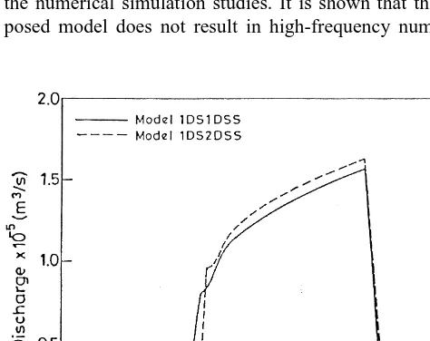
effects are only marginal and the application of the simple model 1DS1DSS gives satisfactory results. The models developed in the present work are also applied to simulate the outflow hydrograph for the case shown in Fig. 9(c), in which the subsurface soil characteristics vary in a com-plicated manner. It should be noted here that even the model 1DS1DSS considers the heterogeneity of the sub-surface and there is no homogenization. The only difference between models 1DS1DSS and 1DS2DSS is that in the former case the flow is assumed to be only in the vertical direction. The outflow hydrographs obtained using models 1DS1DSS and 1DS2DSS for the above case are shown in Fig. 13. The effect of two-dimensionality in
the subsurface flow is very much evident in this case. The one-dimensional model shows an early ponding and a reduced peak. It can be concluded from the above simula-tion studies that, in many cases where the groundwater table is very deep, the unsaturated flow in the ground may be considered one-dimensional for the purpose of simulating the overland flow. This assumption is valid, especially when the spatial variation in the soil character-istics is only in the vertical direction. However, two-dimensionality comes into the picture if the spatial varia-tion of the soil characteristics is very complex and is in both x and z directions. Model 1DS2DSS should be used in such cases.
Fig. 10. Effect of simplification of layered subsoil conditions using a single layer on outflow hydrograph.
6 CONCLUSIONS
In this study, a conjunctive surface–subsurface numerical model is developed for the simulation of overland flow. In this model, the complete Saint-Venant equations are solved using a simple, explicit, high-resolution essentially non-oscillating (ENO) finite-difference scheme. The subsurface flow component in the proposed model is represented by the two-dimensional Richards equation in the mixed form. This equation is solved by a recently developed efficient strongly implicit finite-difference scheme. The proposed conjunctive model is verified using experimental data available in the literature. The ability of the proposed model to handle complex subsurface conditions is demonstrated through the numerical simulation studies. It is shown that the pro-posed model does not result in high-frequency numerical
oscillations even for hydrographs with steep rising limbs. It is found from the numerical simulation studies that, in many cases where the groundwater table is deep, the unsaturated flow in the ground may be considered one-dimensional. It is also possible to obtain further simplifica-tion if it is assumed that the infiltrasimplifica-tion rate is more or less uniform. Such an assumption may be valid if the spatial variation in the subsoil characteristics is only in the vertical direction. However, two-dimensional effects do become significant if the spatial variation of the soil characteristics is complex and is in both x and z directions.
ACKNOWLEDGEMENTS
The authors thank Prof. K. Subramanya of I.I.T. Kanpur for the many interesting discussions. They also thank the anonymous reviewers whose comments helped in signifi-cantly improving the quality of this paper.
REFERENCES
1. Abbott, M.B., Computational Hydraulics: Elements of the Theory of Free Surface Flows. Pitman, London, 1985. 2. Abbott, M.B., Bathurst, J.C., Cunge, J.A., O’Connell, P.E.
and Rasmussen, J. An introduction to the European Hydro-logical System—System Hydrologique European, ‘SHE’, 2: Structure of a physically-based distributed modeling system. J. Hydrol., 1986, 87, 61–77.
3. Akan, A.O. Overland flow hydrographs for SCS Type II rain-fall. J. Hydraulic Eng. ASCE, 1985, 111(3), 276–286. 4. Akan, A.O. Similarity solution of overland flow on pervious
surface. J. Hydraulic Eng. ASCE, 1985, 111(7), 1057–1067. 5. Akan, A.O. and Yen, B.C. Mathematical model of shallow water flow over porous media. J. Hydraulic Division, 1981,
107(HY4), 479–494.
6. Alcrudo, F., Garcia-Navarro, P. and Saviron, J.M. Flux dif-ference splitting for ID open channel flow equations. Int. J. Numerical Methods Fluids, 1992, 14, 1009–1018.
7. Allen, M.B. and Murphy, C.L. A finite-element collocation method for variably saturated flow in two space dimensions. Water Resources Research, 1986, 22(11), 1537–1542. 8. Amein, M. An implicit method for numerical flood routing.
Water Resources Research, 1968, 4(4), 719–726.
9. Celia, M.A., Bouloutas, E.F. and Zarba, R.L. A general mass-conservative numerical solution for the unsaturated flow equation. Water Resources Research, 1990, 26(7), 1483– 1496.
10. Cooley, R.L. Some new procedures for numerical solution of variable saturated flow problems. Water Resources Research, 1983, 19(5), 1271–1285.
11. Chaudhry, M.H., Open-channel Flow. Prentice-Hall, Engle-wood Cliffs, NJ, 1993.
12. Chow, V.T. and Ben-Zvi, A. Hydrodynamic modeling of two-dimensional watershed flow. J. Hydraulic Division, 1973, 99(HY11), 2023–2040.
13. De Lima, J.L.M.P. and Van der Molen, W.H. An analytical kinematic model for the rising limb of overland flow on infiltrating parabolic shaped surfaces. J. Hydrol., 1988, 104, 363–370.
14. Freeze, R.A. and Cherry, J.A., Ground Water. Prentice-Hall, Englewood Cliffs, NJ, 1979.
Fig. 12. Comparison of models 1DS1DSS and 1DS2DSS: outflow
hydrograph for case (b) of Fig. 9.
Fig. 13. Comparison of models 1DS1DSS and 1DS2DSS: outflow
15. Govindaraju, R.S., Jones, S.E. and Kavvas, M.L. On the diffusion wave model for overland flow 1. Solution for steep slopes. Water Resources Research, 1988, 24(5), 734– 744.
16. Govindaraju, R.S. and Kavvas, M.L. Dynamics of moving boundary overland flows over infiltrating surfaces at hill-slope. Water Resources Research, 1991, 27(8), 1885–1898. 17. Govindaraju, R.S., Kavvas, M.L. and Tayfur, G. A simplified model for two-dimensional overland flows. Water Resources Research, 1992, 27(8), 1885–1898.
18. Haverkamp, R. and Vauclin, M. A note on estimating finite-difference interblock hydraulic conductivity values for tran-sient unsaturated flow problems. Water Resources Research, 1979, 15(1), 181–187.
19. Hills, R.G., Porro, I., Hudson, D.B. and Wierenga, P.J. Modeling one-dimensional infiltration into very dry soils, 1. Model development and evaluation. Water Resources Research, 1989, 25(6), 1259–1269.
20. Hong, L.D., Akiyama, J. and Ura, M. Efficient mass-conservative numerical solution for the two-dimensional unsaturated flow equation. J. Hydroscience Hydraulic Engi-neering, 1994, 11(2), 1–18.
21. Hromadka, T.V. II, McCuen, R.H. and Yen, C.C. Com-parison of overland flow hydrograph models. J. Hydraulic Eng. ASCE, 1987, 113(11), 1422–1440.
22. Kawahara, M. and Yokoyama, T. Finite element method for direct runoff flow. J. Hydraulic Division ASCE, 1980,
106(HY4), 519–534.
23. Lapidus, A. A detached shock calculation by second order finite differences. J. Computational Physics, 1967, 2, 15–77. 24. Lin, W., Gray, D.M. and Norum, D.I. Hydrodynamics of laminar flow over a porous bed. Water Resources Research, 1973, 9(6), 1637–1644.
25. Morris, E.M. and Woolhiser, D.A. Unsteady one-dimensional flow over a plane: Partial equilibrium and recession hydro-graphs. Water Resources Research, 1980, 16, 355–360. 26. Narasimhan, T.N. and Witherspoon, P.A. Numerical model
for saturated-unsaturated flow in deformable porous media, 3. Applications. Water Resources Research, 1978, 14(6), 1017–1034.
27. Nujic, M. Efficient implementation of non-oscillatory schemes for the computation of free-surface flows. J. Hydraulic Research IAHR, 1995, 33(1), 101–111.
28. Preissmann, A. and Zaoui, J., Le module ‘e´coulement de surface’ due Syste´me Hydrologique Europeen (SHE). In: Proc. 18th Congress of IAHR, Cagliari, 5, 1979, pp. 193– 199.
29. Smith, R.E. and Woolhiser, D.A. Overland flow on an infiltrat-ing surface. Water Resources Research, 1971, 7(4), 899–913. 30. Sunada, K. and Hong, T.F. Effects of slope conditions on
direct runoff characteristics by the interflow and overland flow model. J. Hydrol., 1988, 102, 323–334.
31. Tayfur, G., Kavvas, M.L., Govindaraju, R.S. and Storm, D.E. Applicability of St. Venant equations for 2-D overland flow over rough infiltrating surfaces. J. Hydraulic Eng. ASCE, 1993, 119(1), 51–63.
32. Todini, E., Venutelli, M., Overland flow: A two-dimensional modeling approach. In: Recent Advances in the Modeling of Hydrologic System. Kluwer Academic Publishers, The Netherlands, 1991, pp. 153–166.
33. Vieira, J.H.D. Conditions governing the use of approxima-tions for the Saint-Venant equaapproxima-tions for shallow surface water flow. J. Hydrol., 1983, 60, 43–58.
34. Woolhiser, D.A. and Liggett, J.A. Unsteady one-dimensional flow over a plane—the rising hydrograph. Water Resources Research, 1967, 3(3), 753–771.
35. Yee, H.C., A class of high-resolution explicit and implicit shock-capturing methods. NASA Technical Memorandum 101088, Ames Research Center, CA, 1989.
36. Yen, B.C. Open channel flow equations revisited. J. Eng. Mechanics Division ASCE, 1973, 99(EM5), 979–1009. 37. Zhang, W. and Cundy, T.W. Modeling of two-dimensional