TOWARDS AUTOMATIC SINGLE-SENSOR MAPPING BY MULTISPECTRAL
AIRBORNE LASER SCANNING
E. Ahokas a*, J. Hyyppä a, X. Yu a, X. Liang a, L. Matikainen a, K. Karila a, P. Litkey a, A. Kukko a, A. Jaakkola a, H. Kaartinen a, M. Holopainen b, M. Vastarantab
a
Finnish Geospatial Research Institute FGI, National Land Survey, Masala, Finland – (eero.ahokas, juha.hyyppa, xinlian.liang, xiaowei.yu, leena.matikainen, kirsi.karila, paula.litkey, antero.kukko, anttoni.jaakkola, harri.kaartinen)@nls.fi
b
Helsinki University, HU, Helsinki – (markus.holopainen, mikko.vastaranta)@helsinki.fi
Commission III, WG III/2
KEY WORDS: laser scanning, lidar, multispectral, mapping, automation, intensity, change detection, classification
ABSTRACT:
This paper describes the possibilities of the Optech Titan multispectral airborne laser scanner in the fields of mapping and forestry. Investigation was targeted to six land cover classes. Multispectral laser scanner data can be used to distinguish land cover classes of the ground surface, including the roads and separate road surface classes. For forest inventory using point cloud metrics and intensity features combined, total accuracy of 93.5% was achieved for classification of three main boreal tree species (pine, spruce and birch).When using intensity features – without point height metrics - a classification accuracy of 91% was achieved for these three tree species. It was also shown that deciduous trees can be further classified into more species. We propose that intensity-related features and waveform-type features are combined with point height metrics for forest attribute derivation in area-based prediction, which is an operatively applied forest inventory process in Scandinavia. It is expected that multispectral airborne laser scanning can provide highly valuable data for city and forest mapping and is a highly relevant data asset for national and local mapping agencies in the near future.
* Corresponding author
1. INTRODUCTION
During the last 10 years, intensity calibration of Airborne Laser Scanning (ALS) has progressed from a research idea into an operational practise in ALS systems. The first radiometric calibration methods and their applications were presented by Coren and Sterzai (2006), Ahokas et al. (2006), Wagner et al. (2006), and Höfle and Pfeifer (2007). Physical concepts of laser scanner intensity calibration are depicted in Wagner (2010), and some of the effects related to the resulting scanner intensity record have been experimentally investigated e.g., by Kukko et al. (2008) and Abed et al. (2012). The need for radiometric calibration of the laser scanning (LS) intensity stems from the possibility of using calibrated intensity as an additional feature for object classification and object characteristics estimation. EuroSDR (European Spatial Data Research) hosted a project “Radiometric Calibration of ALS Intensity” during the years 2008-2011, led by FGI and TU Wien, in which radiometric calibration techniques were studied in practise. The major motivation was that “someday, there will be multispectral airborne laser scanning” available and single-sensor applications are possible without the need of merging ALS and passive imaging data.
Our paper reviews first the previous intensity calibration work from the perspective of near future multispectral ALS. What does it mean for the multispectral ALS? Secondly, Optech Titan multispectral ALS data over a large suburban area (south Espoo) and boreal forest area (Evo) in Finland were acquired in August 2015. The dataset includes three channels, and the total point density is between 12 to 25 points/m2. We will show some
of the first results and interpretations with the new data. Characteristics of the new data are reported. Tree species classification, automated mapping of buildings and individual trees, area-based forest inventory, mapping of roads and land cover classes are reported and discussed. Our preliminary analyses suggest that the new data are very promising for further increasing the automation level in mapping, and large variety of single-sensor applications are seen possible.
2. FROM INTENSITY CALIBRATION TO
MULTISPECTRAL LASER SCANNING
In laser scanning, an intensity value is often recorded for each point – in addition to point’s x,y,z information. The intensity represents the momentary measured power or amplitude value of the received pulse for discrete return lasers. With full-waveform lasers, the total received power corresponding to the backscattering cross-section can be calculated from the intensity waveform. Various terms are used in addition to intensity: reflectance, backscatter, brightness because scientists and engineers operating in the field of laser scanning represent different disciplines.
The need for the radiometric calibration of the laser scanning intensity stems from the possibility of using calibrated intensity as additional feature for object classification and object characteristics estimation. Even uncalibrated intensities can be used to register laser scanning and imagery data.
Intensity is affected by target surface characteristics (reflectance and roughness), environmental effects (atmospheric transmittance, moisture), and acquisition parameters and instrument characteristics. Therefore, intensity is influenced by the distance to the target, the angle of incidence, the roughness and reflectance of the target surface, the atmosphere, the transmitted pulse energy, the receiver noise and changes in sensitivity, the wavelength, the pulse width, beam divergence, and the possibly used automatic gain control (AGC). For example, surface wetness affects the Titan 1550 nm channel intensity.
A technical note about intensity can be found in Katzenbeisser (2002). At the same time Swedish TopEye system was already pre-calibrated for range effects on intensity (Sterner, 2001). Waveform radars were already calibrated with similar techniques in the 90’s (e.g. Hyyppä et al., 1999).
Radiometric calibration of laser intensity data aims at retrieving a value related to the target scattering properties, which is independent on the instrument or data acquisition parameters. There are two types of calibration, i.e. relative and absolute calibration.
Relative calibration of ALS intensity means that measurements from different ranges, incidence angles and dates are comparable for the same system. The factors affecting received intensity in the relative calibration are spreading loss, backscattering properties versus incidence angle, transmitter power changes, especially when pulse repetition frequency (PRF) is changed, and atmospheric properties. Since most of the natural materials are rough at laser scanning wavelengths, the effect of incidence angle is mostly indistinguishable within an ALS footprint.
Absolute calibration of ALS intensity means that the obtained corrected value of intensity describes the target properties and corresponding values obtained from various sensors are directly comparable. In absolute calibration, the obtained and relatively corrected intensity values are linked with known values (e.g. backscattering coefficient or reflectance) of the reference objects. The methods useful for absolute calibration include 1) use of tarps (Kaasalainen et al., 2005) or 2) use of gravel or other natural material (Kaasalainen et al., 2009) for which the reflectance/backscattering coefficient is known. The tarps, gravels and natural materials can be measured using e.g. laboratory systems allowing backscattering measurements, calibrated NIR camera operating in the same wavelength region, and calibrated reflectometer. Since in airborne surveys it is unlikely to get simultaneous intensity reference measurements done, it is also possible to assume backscattering properties of objects, for example, based on backscattering library data.
EuroSDR hosted a project “Radiometric Calibration of ALS surface, therefore, this type of calibration can be made with ”only pulses” (first of many, last of many). Intermediate returns are obtained with beams partly seeing multiple targets and even range correction,
thus, is unfeasible to be calibrated without further delve.
2. Meta data should be saved for each flight track 3. Mapping agencies and companies should provide
relatively calibrated intensities for the users as soon as possible, since that should not add the costs. Production of relatively calibrated intensities needs some changes to the processing software, however. 4. In the processing, radiometric strip adjustment is
recommended. Model based correction (based on lidar equation) is recommended to be used for calibration (see e.g. Wagner, 2010, Höfle and Pfeifer, 2007). Overlapping information may be used to minimize variation in the data and to determine constants in the correction formula (Gatziolis, 2011).
In order to classify and characterize the object properly, we can use geometry from point clouds, hyperspectral response and BRF response (illumination geometry known). The major bottleneck in passive multi- or hyperspectral data processing is the illumination change (bidirectional reflectance distribution function, BRDF, Sun movement, clouds) of the environment. The BRDF changes of mobile imagery are even more dramatic than in aerial imaging, since imaging is done in all geometries. Therefore, active multispectral laser scanning seemed to be an attractive solution for future laser scanning. In Hyyppä et al. (2013) it was proposed that 3-4 channel laser scanning system may be feasible for automated object recognition. Additionally, it was proposed that the beam width of each channel may differ giving different information from targets.
3. MATERIAL
3.1 Titan airborne laser scanner
Optech Titan is the first commercial three channel airborne laser scanner. The spectral channels are two infrared ones, IR (1550 nm) channel 1, NIR (1064 nm) channel 2, and green (532 nm) channel 3. The green channel is suitable for shallow clear water bathymetry applications up to 15 m depth. Operating altitudes for the three channels are 300-2000 m above ground level for topographic applications and 300-600 m for bathymetric applications using the green channel. According to the manufacturer’s specifications horizontal accuracy is 1/7500 x altitude (in 1 s) and elevation accuracy is <5-10 cm (in 1 s) for 1064 nm and 1550 nm channels. Beam divergence (1/e) is 0.35 mrad for NIR and IR channels and 0.7 mrad for the green channel. Effective pulse repetition frequency is 900 kHz total (300 kHz per channel). The scan pattern of Titan is such that 1064 nm channel is scanning 0 degrees down, 1550 nm channel is pointing 3.5 degrees forward, and 532 nm channel is pointing 7 degrees forward. Laser pulses are not registered exactly from the same point in each channel. When the green channel of Titan is applied to bathymetric applications e.g. the depth of water, reflectance of seabed, refraction and attenuation coefficients of water have to be taken into account.
3.2 Test sites
Optech Titan campaigns in Finland were carried out in two places, on the southern coast in the city of Espoo and in the Evo test area that is located in Southern Finland, some 100 km north of Helsinki. Evo is a boreal forest site. A detailed description of the Evo study area can be found in Yu et al. (2015). The average stand size is less than 1 ha in this managed boreal forest The International Archives of the Photogrammetry, Remote Sensing and Spatial Information Sciences, Volume XLI-B3, 2016
covering about 2000 ha. The proportion of Scots pine (Pinus sylvestris) is 40%, that of Norway spruce (Picea abies) is 35%, and that of deciduous trees (mainly birch, Betula spp.) is 24% of the total stem volume. The altitude of the site varies between 125 m and 185 m above sea level. Four field plots (32 m × 32 m, 1024 m2) having 215 trees were used for tree species classification. Sample plot locations were determined using the geographic coordinates of the plot center and four corners. Plot center positions were measured using a total station (Trimble 5602), which was oriented to local coordinate system using ground control points measured with VRS-GNSS (Trimble R8) on open areas close to the plot. Terrestrial laser scanning (TLS) measurements were carried out and tree maps were created based on TLS data. These tree maps were used for visual tree species mapping.
3.3 Data collection
The details of the two test flights in Finland of sensor L349 are depicted below in Table 1. The date of flight in Espoo was 21st and in Evo 24th August, 2015.
Locati on
Flying height (m)
PRF (kHz)
Scan rate (Hz)
FOV (°)
Point density (pts/m2)
Strip width (m) Espoo 650 3x200 40 40 3 x 6 473 Evo 400 3x300 53 30 3 x 21 214
Table 1. Optech Titan data collection test flights.
Side/lateral overlap was 20 %.
3.4 Data pre-processing
The data were pre-processed as follows. TerraTec AS, Norway, made the processing of the GPS/INS data using TerraPOS software, and the basic data processing using Optech system software. TerraTec Oy, Finland, made the geoid correction to N2000 system using the geoid model Fin2005. Matching of the flight strips was carried out using TerraMatch software. The original data had ground point classification for some flight lines or tiles, this was for channel 2. In the processing of Evo data at the FGI, ground point classification was computed for all files in channel 2 with LasTools lasground_new function using default settings. Relative intensity calibration was made at the FGI using R2 correction in Espoo and R2.5 correction for the forest areas in Evo.
4. APPLICATIONS
4.1 Land cover classification
Land cover classification was tested in a 4 km2 suburban area in Espoonlahti, Espoo. An object-based approach using a digital surface model (DSM) and intensity image in raster format was used. The method included segmentation of high objects (height above ground > 2.5) on the basis of the DSM and segmentation of low objects on the basis of the intensity image. High objects were further classified into buildings or trees, and low objects were classified into asphalt, gravel, rocky areas or low vegetation. The classification was based on the Random Forests (RF) method (Breiman, 2001). The importance of various features was estimated, and out-of-bag classification errors were calculated on the basis of reference points. The numerical results and details of the study are presented in Matikainen et al.
(2016). Figures 2 to 6 show the classification results for five subareas.
It can be seen that the general appearance of the classification results is satisfactory. In addition to classifying high objects, the multispectral laser scanner data can be used to distinguish land cover classes of the ground surface. For example, the main roads have been mainly recognized as asphalt-covered surfaces. Many narrow walkways have been correctly classified as gravel. The data also seems promising for the mapping of bare rock areas. Naturally, some classification errors also occurred. The most remarkable of these were bridges classified as buildings. This is related to the clear height difference between the DSM and a digital terrain model (DTM) for these objects. Further development should include more advanced methods to avoid such errors. More classes should also be included in the analysis, such as poles, cars, and more detailed land cover classes.
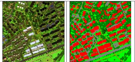
Figure 1. Legend of classified images in Figures 2 to 6. Class
High object includes a few very small segments that remained
unclassified in further building/tree classification.
Figure 2. Optech Titan colour coded RGB image in which Red is Ch1, Green is Ch2, and Blue is Ch3 (left) and classified image (right).
Figure 3. Optech Titan colour coded image (left) and classified image (right).
Figure 4. Optech Titan colour coded image (left) and classified image (right).
Figure 5. Optech Titan colour coded image (left) and classified image (right).
Figure 6. Optech Titan colour coded image (left) and classified image (right).
4.2 Road mapping
Visual analysis of the multispectral intensity images and results of the land cover classification suggest that the Titan data are very promising for automated road mapping (see Figure 7). This topic was studied further, and the preliminary results of this more specific analysis are reported in this section.
A road mapping test was carried out in the Espoonlahti study area (4 km2). First, multiresolution segmentation of the Titan intensity data (20 cm raster) was performed using eCognition software (Trimble Germany GmbH, Munich). Segment-based classification was carried out using Matlab’s (The Mathworks, Inc., Natick, MA, USA) RF implementation. Segment attributes included intensity and height mean and standard deviation values, intensity channel ratios, intensity 25/50/75 % quantiles, normalized difference vegetation index (NDVI) (from NIR and green channels), min and max intensity values and height difference between DSM and DTM. The training data comprised of 365 road points (227 asphalt, 138 gravel) and 333 points for the class ‘other’. For each point the corresponding segment was extracted. The classification was carried out in two phases; 1) road detection (road/other), 2) asphalt/gravel classification. Two RF models were constructed using the training data.
Validation points were created in parts of the study area not covered by training data using road data from the topographical database. A total of 1934 test points (of them 397 were on gravel roads) were created along the road vectors every 10 meters. Predictions were made based on the RF models created using the training data. A percentage of 70.9% of the road test points were classified as roads. Principally, roads were not detected due to trees covering the roads since leaves were on trees during data acquisition. For 85.8 % of the points classified as road the surface was classified correctly as asphalt or gravel.
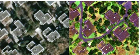
Figure 7. Aerial image ©NLS (left) and Titan intensity image (right).
4.3 Forest inventory and tree species classification
In terms of the ratio of forest cover to total land area, Finland and Sweden are the world’s most extensively forested countries among the industrialized and temperate countries (73% and 69% of the land area), the corresponding value of Norway is 37%. The Nordic Countries Finland, Norway and Sweden, are among the most important producers of timber and other forest products in the world. In Finland and Sweden, the forest sector accounts for significant share of export revenue and acts as a major employer especially in regional areas. Volume of Nordic forest resources is 5600 million cubic meters and annual increment about 220 million cubic meters, out of which 150 million cubic meters is harvested. In the Nordic Countries we have more than 300 billion trees in our forests.
In 3D remote sensing, forest attributes estimation includes typically the following steps (Hyyppä et al., 2015). DTM is first obtained from ALS data. Canopy Height Model (CHM) is calculated to get tree heights and tree height metrics. Features (point cloud metrics) are calculated from the data, and typically non-parametric estimation (e.g. k-NN, RF) is applied. Non-parametric estimation requires field plots, which are used for model building. In addition to the point cloud metrics, other features, such as individual-tree information, texture, waveform laser scanning features, image processing applied to e.g. DSMs, image-based features (including NDVI), and other channel information and ratios, can be added to improve the prediction. Species-specific forest attributes are predicted, and therefore, the system should include features capable to discriminate species. The optimum output, requested by forest companies of the process is species-specific size (dbh, height) distribution of the trees. The current species-specific forest inventory attributes and diameter distributions have poor prediction accuracy and errors at the level of 50% or higher. Therefore, the first tree species classification for forest inventory purposes was studied using Optech Titan. The objective is to get reliable classification for pine, spruce and deciduous trees.
Data analysis was conducted in six steps: 1) co-registration among the datasets to remove the possible displacements, 2) creation of CHM from Titan, 3) individual tree detection, Figure 8, 4) tree feature calculation using intensity, Figure 9, 5) tree species estimation using RF method and 6) validation of the data with out-of-bag sample. Canopy height was calculated with 0.5 m pixel size from all points of three channels. Locations of all trees on the TLS tree map were used to help find the true location of the plot with respect to the ALS point cloud. The plot was shifted and rotated so that the tree locations within the map properly aligned with the point cloud. Individual trees were detected using a minimum curvature-based region detector (Yu et al., 2011). The method is a raster image-based algorithm. First, a raster CHM was created from normalized data for each plot. CHM was then smoothed by applying a Gaussian filtering. The International Archives of the Photogrammetry, Remote Sensing and Spatial Information Sciences, Volume XLI-B3, 2016
Single-tree segmentations were finally performed on smoothed CHM images using a minimum curvature-based region detector. For each detected tree, intensity features were calculated from each channel separately, including minimum, maximum, mean, standard deviation, range, skewness and kurtosis of intensity, percentiles of intensity at 5% and from 10% to 90% with 10% increment. RF was used to select 15 most important features out of 54 ones. With selected features as predictors, classification was carried out using RF, which is a non-parametric regression technique using multiple number of classification trees (Breiman, 2001). The samples that are not used in training are called “out-of-bag” observations, which can serve as testing data in cross-validation. Prediction made for out-of-bag observations are called out-of-bag prediction. Thus, results were analysed based on out-of-bag predictions and compared with the field reference data.
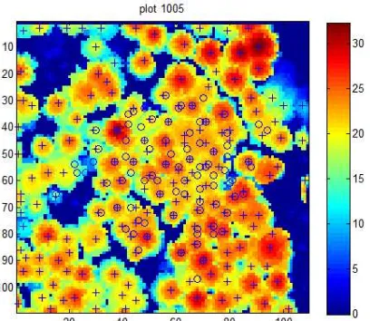
Figure 8. Individual tree detection for one of the plots.
Figure 9. Calibrated intensity maps for the same plot using channel 1, channel 2 and channel 3. The beam size in channel 3 is bigger than in the other channels.
The confusion matrix of classification was calculated based on intensity features of all returns (Table 2), on intensity features of first returns (Table 3) and on intensity features and point cloud features of first returns (Table 4). In these Tables, best 15 features were used. With point cloud and intensity features combined, the results were also calculated without selection of 15 best features (Table 5).
Predicted
Pine Spruce Birch
Reference Pine 97 1 3
Spruce 1 45 6
Birch 2 6 55
Table 2. Confusion matrix of classification based on intensity features of all returns with 15 best features. Total accuracy is 91.2%.
Predicted Pine Spruce Birch
Reference Pine 97 2 2
Spruce 1 44 6
Birch 2 6 55
Table 3. Confusion matrix of classification based on intensity features of first returns with 15 best features. Total accuracy is 91.2%.
Predicted Pine Spruce Birch
Reference Pine 97 2 2
Spruce 1 43 7
Birch 3 5 55
Table 4. Confusion matrix of classification based on intensity features and point cloud features of first returns with 15 best features. Total accuracy is 90.7%.
Predicted
Pine Spruce Birch
Reference Pine 97 1 3
Spruce 0 48 3
Birch 2 5 56
Table 5. Confusion matrix of classification based on intensity features and point cloud features of first returns. Total accuracy: 93.5%.
The accuracy providing tree species of 90% accuracy at tree level is better than with digital aerial images. The results propose a significant potential for operative forest inventory. By adding waveform features, such as echo width, it is expected to improve the accuracies even from this.
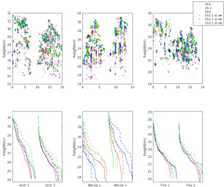
Secondly, we studied point distributions in deciduous species Betula sp, Tilia x vulgaris and Acer platanoides. Therefore, we studied two trees per each species in Espoo, Figure 10. The city of Espoo provided their urban tree map including species information for reference material. Trees located along the The International Archives of the Photogrammetry, Remote Sensing and Spatial Information Sciences, Volume XLI-B3, 2016
streets and in parks. Acer platanoides has broad leaves and pulses of all channels are reflecting from the surface without much penetration inside. Cumulative height distribution of Tilia x vulgaris has a compact form, too. Betula pendula has smaller leaves than Acer platanoides and pulses penetrate inside the tree. It should be reminded that the footprint size of Channel 3 is double compared to that of channels 1 and 2. The number of points per channel has been normalized by dividing channel wise number of points by the channel with most points. The structure of different tree species seems to be different in each deciduous tree species, and multispectral ALS shows great potential for further classification of tree species.
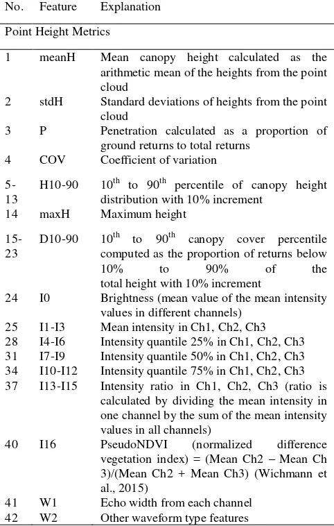
Thirdly, the prediction of stand variables is typically based mainly on point height metrics calculated from ALS data. Already in 1988, Nelson et al. divided features related to the height and density, which is the current foundation of the area-based technology. Features such as percentiles calculated from a normalized point height distribution, mean point height, densities of the relative heights or percentiles, standard deviation, and coefficient of variation are generally used. We are proposing that intensity-related features and waveform-type features are added to the standard list of point height metrics usable for forest attribute derivation, as listed in Table 6 as an example. Several percent improvements in the prediction accuracy can be achieved in such a process.
No. Feature Explanation
Point Height Metrics
1 meanH Mean canopy height calculated as the arithmetic mean of the heights from the point cloud
2 stdH Standard deviations of heights from the point cloud
3 P Penetration calculated as a proportion of ground returns to total returns
4 COV Coefficient of variation
5-computed as the proportion of returns below
10% to 90% of the
Brightness (mean value of the mean intensity values in different channels)
Mean intensity in Ch1, Ch2, Ch3 Intensity quantile 25% in Ch1, Ch2, Ch3 Intensity quantile 50% in Ch1, Ch2, Ch3 Intensity quantile 75% in Ch1, Ch2, Ch3 Intensity ratio in Ch1, Ch2, Ch3 (ratio is calculated by dividing the mean intensity in one channel by the sum of the mean intensity values in all channels) useful for land cover classification, also when considering ground surface objects and classes, such as roads, and reaching an estimate for classification error about 3% for separating classes asphalt, gravel, rocky areas and low vegetation from each other. Matikainen et al. (2016) also propose that the new data are very promising for further increasing the automation level in mapping.
In addition to classifying high objects, the multispectral laser scanner data can be used to distinguish land cover classes of the ground surface, including the roads. For forest inventory using point cloud metrics and intensity features combined, total accuracy of 93.5% was achieved for pine, spruce and birch classification. When using simple intensity features of first or all returns – without point height metrics - a classification accuracy of 91% was achieved for main boreal tree species. It was shown that deciduous trees can also be further classified into more classes. We proposed that intensity-related features and waveform-type features are added to standard list of point height metrics usable for forest attribute derivation in area-based prediction, which is an operatively applied forest inventory process in Scandinavia.
One major lack with applied Titan data was the inhomogeneity of the point cloud. In the across track, the point spacing was significantly smaller than in the along track direction. Either lower aircraft speed of higher scan frequency should be achieved to provide more homogenous point spacing.
Multispectral airborne laser scanning offers a tool for automatic single-sensor mapping. An increased automation level in forestry and mapping applications are certainly possible in the future. It is expected that multispectral airborne laser scanning can provide highly valuable data for city and forest mapping and is a highly relevant data asset for national and local mapping agencies in the near future.
ACKNOWLEDGEMENTS
The research leading to these results has received funding from Academy of Finland projects “Interaction of Lidar/Radar Beams with Forests Using Mini-UAV and Mobile Forest Tomography” (No. 259348), and “Centre of Excellence in Laser Scanning Research (CoE-LaSR)” (No. 272195) and Tekes RYM Oy Research Programme “Energizing Urban Ecosystems”, and “Integration of Large Multisource Point Cloud and Image Datasets for Adaptive Map Updating” (No. 295047), and in part the research leading to these results has received funding from the European Community's Seventh Framework Programme ([FP7/2007-2013]) under grant agreement n° 606971.
REFERENCES
Abed, F., Mills, J., Miller, P., 2012. Echo Amplitude Normalization of Full-Waveform Airborne Laser Scanning Data Based on Robust Incidence Angle Estimation. IEEE
Transactions on Geoscience and Remote Sensing. Vol. 50, No
7, pp. 2910-2918.
Ahokas, E., Kaasalainen, S., Hyyppä, J., Suomalainen, J., 2006. Calibration of the Optech ALTM 3100 laser scanner intensity data using brightness targets. ISPRS Commission I Symposium, Paris Marne-la-Vallee, 4-6 July 2006, ISPRS Volume XXXVI Part 1/A. pp. 14-20. CD-ROM publication.
Breiman, L., 2001. Random forests. Mach. Learn., Vol. 45, pp. 5–32.
Coren, F., Sterzai, P., 2006. Radiometric correction in laser scanning. International Journal of Remote Sensing. Vol. 27, No. 15-16, pp. 3097-3104.
Gatziolis, D. (2011): Dynamic range-based intensity normalization for airborne, discrete return lidar data of forest canopies. Photogrammetric Engineering & Remote Sensing. Vol. 77, No 3: pp. 251-259.
Hyyppä, J., Mäkynen, M., Hallikainen, M., 1999. Calibration accuracy of the HUTSCAT airborne scatterometer. IEEE
Transactions on Geoscience and Remote Sensing, Vol. 37, No.
3, pp. 1450-1454.
Hyyppä, J., 2011. State of the Art in Laser Scanning. In:
Photogrammetric Week'11, ed. by Dieter Fritsch. Wichmann
Verlag, VDE VERLAG GMBH, Berlin and Offenbach. ISBN 978-3-87907-507-2, pp. 203-216.
Hyyppä, J., Jaakkola, A., Chen Y., Kukko, A., Kaartinen, A., Zhu, L., Alho, P., Hyyppä, H., 2013. Unconventional Lidar mapping from air, terrestrial and mobile. In: Photogrammetric
Week'13, ed. by Dieter Fritsch.
http://www.ifp.uni-stuttgart.de/publications/phowo13/180Hyyppae.pdf
Hyyppä, J., Karjalainen, M., Liang, X., Jaakkola, A., Yu, X., Wulder, M., Hollaus, M., White, J.C., Vastaranta, M. and Karila, K., Kaartinen, H., Vaaja M., Kankare, V., Kukko, A., Holopainen, M., Hyyppä, H., Katoh. M., 2015. Remote Sensing of Forests from Lidar and Radar. In Land Resources Monitoring, Modeling, and Mapping with Remote Sensing, Editor Thenkabail, pp. 397-427. CRC Press.
Höfle, B., Pfeifer N., 2007. Correction of laser scanning intensity data: Data and model-driven approaches. ISPRS
Journal of Photogrammetry and Remote Sensing, Vol. 62, No.
6, pp. 415-433.
Kaasalainen, S., Hyyppä, J., Mielonen, T., 2005. Laboratory calibration of backscattered intensity for laser scanning land targets. Proceedings of ISPRS Workshop Laser Scanning 2005, September 12-14, 2005, Enschede, The Netherlands, International Archives of Photogrammetry, Remote Sensing and
Spatial Information Sciences, Vol. XXXVI, Part 3/W19, 13-17,
CD-ROM.
Kaasalainen, S., Hyyppä, H., Kukko, A., Litkey, P., Ahokas, E., Hyyppä, J., Lehner, H., Jaakkola, A., Suomalainen, J., Akujärvi, A., Kaasalainen, M., Pyysalo, U., 2009. Radiometric Calibration of LIDAR Intensity With Commercially Available
Reference Targets. IEEE Transactions on Geoscience and
Remote Sensing. Vol. 47, No. 2, pp. 588-598.
Katzenbeisser, R., 2002. Intensity. Technical note. TopoSys GmbH Ravensburg. http://www.toposys.com/pdf-ext/Engl/ TN-Intensity.pdf
Kukko, A., Kaasalainen, S., Litkey, P., 2008. Effect of incidence angle on laser scanner intensity and surface data.
Applied Optics. Vol. 47. No. 7, pp. 986-992.
Matikainen, L., Hyyppä, J., Litkey, P., 2016. Multispectral airborne laser scanning for automated map updating. In: International Archives of Photogrammetry, Remote Sensing and
Spatial Information Sciences, ISPRS Congress, Prague, Czech
Republic.
Nelson, R., Krabill, W., Tonelli, J., 1988. Estimating forest biomass and volume using airborne laser data. Remote Sensing
of Environment, Vol. 24, pp. 247-267
Sterner, Håkan, 2001. Personal communication.
Wagner, W., 2010. Radiometric calibration of small-footprint full waveform airborne laser scanner measurements: Basic physical concepts. ISPRS Journal of Photogrammetry and
Remote Sensing, Vol. 65, pp. 505-513.
Wagner, W., Ullrich, A., Ducic, V., Melzer, T., Studnicka, N., 2006. Gaussian decomposition and calibration of a novel small-footprint full-waveform digitising airborne laser scanner. ISPRS
Journal of Photogrammetry and Remote Sensing, Vol. 60, No.
2, pp. 100-112.
Wichmann, V., Bremer, M., Lindenberger, J., Rutzinger, M., Georges, C., Petrini-Monteferri, F., 2015. Evaluating the potential of multispectral airborne lidar for topographic mapping and land cover classification. In: ISPRS Annals of Photogrammetry, Remote Sensing and Spatial Information
Sciences, La Grande Motte, France, Vol. II-3/W5, pp. 113-119.
Yu, X. Hyyppä, J. Vastaranta, M. Holopainen, M. Viitala, R., 2011. Predicting individual tree attributes from airborne laser point clouds based on the random forests technique. ISPRS J.
Photo-gramm., Vol. 66, pp. 28–37.
Yu, X., Hyyppä, J., Karjalainen, M., Nurminen, K., Karila, K., Vastaranta, M., Kankare, V., Kaartinen, H., Holopainen, M., Honkavaara, E., Kukko, A., Jaakkola, A., Liang, X., Wang, Y., Hyyppä, H., Katoh, M., 2015. Comparison of Laser and Stereo Optical, SAR and InSAR Point Clouds from Air-and Space-Borne Sources in the Retrieval of Forest Inventory Attributes.
Remote Sensing. Vol 7, No 12, pp. 15933-15954.
Figure 10. Side view and cumulative height distribution of pulses reflecting from deciduous trees, Acer platanoides, Betula pendula, and Tilia x vulgaris in three channels. Channel 1 is indicated in red colour, channel 2 in blue, and channel 3 in green, correspondingly. Little dots are intermediate or last pulses and bigger dots are first or only pulses. Side view of trees (upper row) and cumulative height distribution (lower row). 1st pulse data are in dashed lines. Intermediate and last pulses are in solid lines.