COMPARISON OF UAV-ENABLED PHOTOGRAMMETRY-BASED 3D POINT CLOUDS
AND INTERPOLATED DSMs OF SLOPING TERRAIN FOR ROCKFALL HAZARD
ANALYSIS
J. Manousakis a*, D. Zekkos b, H. Saroglouc, M. Clarkd a
ElxisGroup, Athens, Greece - [email protected] b
Department of Civil and Environmental Engineering, University of Michigan, Ann Arbor, MI – [email protected] c
Department of Civil Engineering, National Technical University of Athens – [email protected] d
Department of Earth and Environmental Science, University of Michigan, Ann Arbor, MI – [email protected]
KEY WORDS: Drones, UAV, Photogrammetry, 3D point clouds, Rockfall, Structure-from-Motion, DSM
ABSTRACT:
UAVs are expected to be particularly valuable to define topography for natural slopes that may be prone to geological hazards, such as landslides or rockfalls. UAV-enabled imagery and aerial mapping can lead to fast and accurate qualitative and quantitative results for photo documentation as well as basemap 3D analysis that can be used for geotechnical stability analyses. In this contribution, the case study of a rockfall near Ponti village that was triggered during the November 17th 2015 Mw 6.5 earthquake in Lefkada, Greece is presented with a focus on feature recognition and 3D terrain model development for use in rockfall hazard analysis. A significant advantage of the UAV was the ability to identify from aerial views the rockfall trajectory along the terrain, the accuracy of which is crucial to subsequent geotechnical back-analysis. Fast static GPS control points were measured for optimizing internal and external camera parameters and model georeferencing. Emphasis is given on an assessment of the error associated with the basemap when fewer and poorly distributed ground control points are available. Results indicate that spatial distribution and image occurrences of control points throughout the mapped area and image block is essential in order to produce accurate geospatial data with minimum distortions.
* Corresponding author
1. INTRODUCTION - UAV APPLICATION FOR ROCKFALL HAZARD ANALYSIS
Unmanned aerial vehicles (UAVs) are expected to be particularly valuable to define topography of natural slopes that may be prone to geological hazards (Niethammer et al. 2012, Murphy et al. 2014, Greenwood et al. 2016, Zekkos et al. 2016). Especially in the case of a landslide or rockfall, the affected area is commonly inaccessible to ground-based field reconnaissance and survey. Ground based field characterization, including traditional land surveying is, in some of these cases, dangerous, time consuming, expensive and not easily repeatable. Satellite imagery may be too expensive and may not be of adequate resolution, depending on project requirements. On the other hand, UAV-enabled imagery and mapping can lead to fast and accurate qualitative and quantitative results for photo documentation as well as basemap analysis that can be used for geotechnical stability analyses.
In this contribution, the case study of a rockfall near Ponti village that was triggered during the November 17th 2015 Mw 6.5 earthquake in Lefkada, Greece is presented with a focus on the 2D/3D basemap development for use in rockfall analyses. A quadrotor UAV was used to collect optical imagery in order to extract 3D terrain data and orthophotos to support the subsequent geotechnical analyses. Emphasis is given on an assessment of the error associated with the basemap when fewer and poorly distributed ground control points are available.
2. SPECIFICATIONS OF 2D/3D FOR ROCKFALL ANALYSIS
Typically, rockfall analysis in 2D relies on the topography accuracy along a specific section of the slope. A resolution of 5 m × 5 m is generally acceptable for two-dimensional analysis. The main disadvantage of 2D analysis is that the influence of the topographic relief on rock trajectories is not taken into account.
For this reason, the use of three-dimensional (3D) rockfall analysis is preferred. The main advantage of 3D analysis is that it may reveal rock trajectories that are not easily detected in the field. Analysis in 3D relies mostly on the accuracy of the Digital Elevation Model (DEM), as the trajectory of the propagating rock blocks can be significantly affected by slope irregularities and deviations can occur with changing slope dip and dip direction.
The spatial precision of the rasterised DEM, which is necessary for 3D rockfall analysis and the accuracy of the simulated kinematics decrease with increasing cell size in the raster map. The preferred resolution of the DEM lies between 2 m × 2 m and 10 m × 10 m (Dorren and Heuvelink, 2004). Experience has shown that a 1 m × 1 m resolution does not necessarily improve the quality while it increases the amount of data substantially.
3. CASE STUDY: ROCKFALL NEAR PONTI VILLAGE
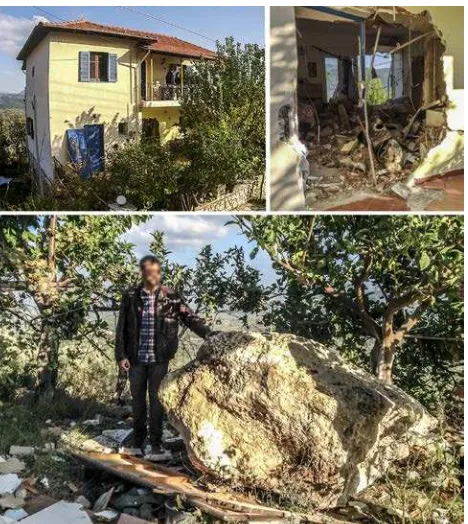
travel path of the rock block, about 800 m in plan view, from the point of detachment to the end of its path. The rock block, near the end of its course, impacted a residential house, penetrated two brick walls, hit and killed a person in the house, exited the house and came to rest in the property’s backyard (Fig. 1).
Figure 1. View of the rock block, the house it impacted near the end of its trajectory and the damage to infill walls that it caused.
Members of the research team reached the study area just two days after the earthquake as part of a reconnaissance expedition. The team’s objective at the time was to identify the origin of dislocation of the rockfall and trace down its path along the sloping terrain and the house. A drone with a high definition (HD) camera was deployed to reach the inaccessible, steep and vegetated uphill terrain and through its virtual First Person View identify the origin of the rock (as shown in Fig. 2) as well as its path.
Figure 2. Aerial oblique view of rockfall origin
In a subsequent expedition, aerial video imagery was collected to produce a high resolution orthophoto of the rockfall trajectory. In addition to mapping the trajectory itself and creating a detailed DSM that can be used as base model to
perform rockfall analysis, of interest was the identification of the route section that the rock rolled versus the sections that the rock bounced. For this purpose, 4K video was captured manually along a gridded path and Structure-from-Motion (SfM) was executed to create a 3D point cloud of the terrain. SfM combines the benefits of photogrammetry and computer vision to reconstruct a 3D scene by identifying matching features in multiple images. These features are tracked image by image, enabling initial estimates of camera positions and object coordinates in an arbitrary 3D coordinate system, which are then refined iteratively using non-linear least-squares minimisation (Westoby et al., 2012). A sparse bundle adjustment (Snavely et al., 2008), needed to transform measured image coordinates into 3D points covering the area of interest, is used in this process. The result is three-dimensional locations of the feature points in the form of a sparse point cloud in the same local 3D coordinate system (Micheletti et al., 2015). Fast-static GPS measurements of 10 control points at the top, middle and bottom surveyed area were introduced to accurately establish internal and external camera parameters and georeference information of the 3D model.
4. DIGITAL GEOSPATIAL RESULTS
4.1 High-resolution Orthophoto
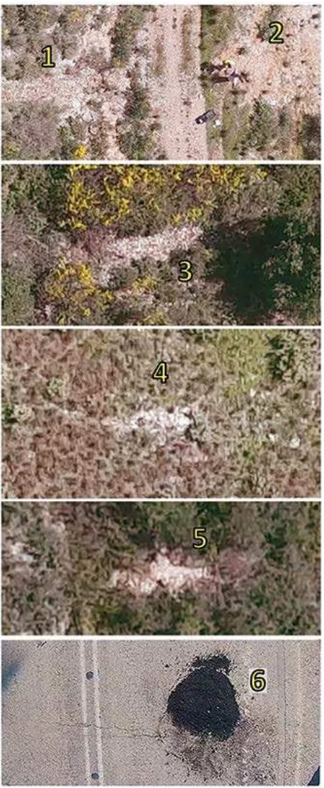
Processing high resolution image sequences through SfM photogrammetry software, a 5cm pixel size orthophoto was produced and was used to identify the rolling section and the bouncing points of the rock throughout its entire course (shown in Fig. 3 and Fig. 4). The rolling section of the rockfall path is distinguished by a destructive linear feature through densely vegetated terrain which alters its colouring with a bare earth tint. In contrast, bouncing impact points stand up as ellipsoidal bare earth craters with no linear traces connecting them. The final bouncing point before impact on the house walls is clearly visible on the asphalt road. Top view ortho-imagery proved to be invaluable for these qualitative assessments. Traditional field reconnaissance and measurements would have been nearly impossible to execute through the steep sloped and vegetated terrain.
4.2 Digital Surface Model
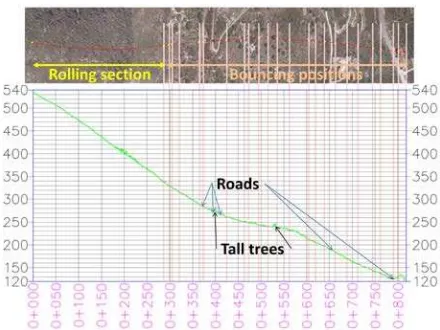
The dense 3D point cloud generated by the SfM processing of the image sequences was interpolated and a Digital Surface Model (DSM) of the terrain was produced. A 10 cm DSM and a profile section of the rockfall path in correlation to the top view orthophoto were originally developed. This DSM was found to be of unnecessarily high resolution that not only was difficult to manipulate in subsequent rockfall analyses, but was also creating numerical problems. Thus, the DSM was downscaled to 2 m for the rockfall analysis, which is still higher resolution than the ground surfaces commonly used in rockfall analyses. The high-resolution DSM made it possible to identify terrain features such as high trees, and structures or benches that could potentially affect the rock’s path downhill (Fig. 5). For rockfall analyses, a 2 m resolution Digital Elevation Model (DEM) was also generated from the 10 cm DSM, by applying aggregate generalization where each output cell contains the minimum of the input cells that are encompassed by the extent of that cell followed by noise filtering and smoothing processing in order to reduce the effect of vegetation and construction elements in the final rasterized product.
Figure 3. Top view orthophoto – Rolling section and bouncing positions recognition
Figure 5. Profile view of rockfall path (units in m)
5. 3D POINT CLOUD ERROR ASSESSMENT FOR DIFFERENT CONTROL POINT SCENARIOS
Spatial accuracy of 3D Point Clouds, DSMs and orthophotos generated by SfM photogrammetry processing is always affected by the ability of the software’s image processing routines to automatically calculate interior and exterior parameters of the camera and images used. Camera calibration and orientation results can further be optimized by introducing to the calculations accurately measured ground control points. In many realistic scenarios of UAV mapping following natural disasters, it may be impossible to collect an ideal number of spatially distributed ground control points of the target of interest for model development. The error in the developed 3D Point Cloud for such cases is a function of a number of factors generally depending on the image quality and camera settings as well as the flight plan and amount of image overlap (James, 2014).
Thus, total images acquisition quality and the results of the camera’s interior orientation with and without the use of ground control points were evaluated. Tie points filtering was introduced after initial photo alignment in order to remove the weakest points in the solution, which have poor base: distance ratios, are wrongly reprojected or are detected on only two photos. As shown in Figure 6, ten (10) ground control points (GCPs) were marked and measured, with fast-static GPS survey, at the top, middle and bottom of the area mapped. Depending on the number and distribution of control points utilized for camera optimization and georeference of the 3d point cloud and DSM extracted from it, the following scenarios were considered:
a) DSM with 6 GCPs distributed at the top, middle and bottom of the target slope.
b) DSM with three GCPs at the top of the target slope. c) DSM with four GCPs at the middle of the target slope. d) DSM with three GCPs at the bottom of the target slope. e) DSM with all ten GCPs used for proper scaling and
geo-positioning, not for camera internal and external parameters optimization.
The remaining of the control points not used for each scenario, were used as check points (CP) to estimate spatial errors of the models.
The auto-calibration and bundle adjustment processes executed for each case scenario produced sparse point cloud models with calculated image tie points RMS reprojection error of 0.80 –
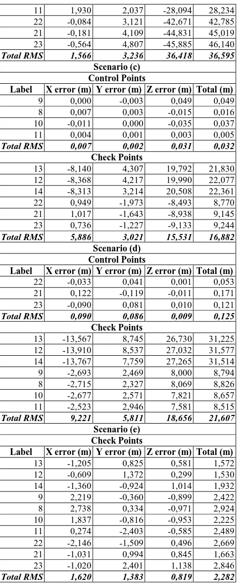
0.90 pixels. Reprojection error refers to the distance between the point on the image where a reconstructed 3D point can be projected and the original projection of that 3D point detected on the photo and used as a basis for the 3D point reconstruction procedure. RMS reprojection error averaged over all tie points on all images used in the project. Sub-pixel results indicate that automatic tie points are identified and positioned with acceptable accuracy and automatic image calibration and alignment produce a good quality 3D reconstructed model. Τhe GCPs and CPs individual errors and total RMS errors in X, Y and Z plane shown in Table 1 for each case scenario demonstrates the impact of using fewer, poorly distributed GCPs on the spatial accuracy and distortion of the final digital terrain product. Note that GCPs 21, 22, 23 located at the bottom of the slope were not properly marked on the ground and the chosen natural details measured with the GPS could not be accurately identified on the UAV images and consequently produce a larger error than the other more precisely positioned GCPs.
Figure 6. Ground Control Points distribution (units in m)
Scenario (a)
11 1,930 2,037 -28,094 28,234
Table 1. GCP and CP errors for different scenarios
Spatial analysis statistics were also calculated to demonstrate the difference between the 6 GCP calibrated DSM and the ones from the different scenarios. The resulting figures are presented for different scenarios accuracy comparison along with statistical metrics of MIN, MAX, MEAN and STD. DEV. values followed by histograms with normal distribution fitting curve on distance differences. For the comparison procedure we utilized CloudCompare. This software uses a distance measurement between point clouds, or meshes, based on a Hausdorff distance (distance based on nearest neighbor)
(Giradeau-Montaut et al. 2004). The Hausdorff distance indicates how far two subsets of a metric space are from one another. It can be defined as the greatest distance from a point in one set to the closest point in the other. Sampled at every point on a surface (point cloud or mesh), it is a generalized approach that is easily automated. This makes it particularly suited for determining the similarity of three dimensional objects, such as those described in this paper. (Cryderman, 2014).
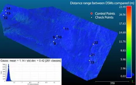
Figure 7 illustrates the reference surface (scenario a) and Figures 8 to 11 show the spatial statistics of each comparison scenario along with normal curve fitting on distance differences according to mean and standard deviation values for each scenario comparison. First, the error (defined as the difference in elevation between the model that is being considered and the model with the 6 GCP included) shown in Fig. 8 - 10 is minimized in the vicinity of the GCPs, but then increases progressively away from the GCPs. Not surprisingly, errors increase with increasing distance from the GCPs. Thus, the spatial distribution of the GCPs is critical. In the scenarios where GCPs are available at the one end of the model (top or bottom of slope), the error in general is higher than in the scenario where the GCPs are at the center of the model. It is important to note though, as presented in Figure 11, that the 3D model geometry in scenario (e), as produced by initial image parameters directly from UAV telemetry and on-board GPS image location is similar and does not suffer from critical deformations and distortions when compared to scenario (a) with the 6 GCP calibrated model. This is also supported by the fact that the distance difference values for scenario (e) follow the normal distribution model.
Figure 7. Scenario (a) – 6 GCPs distributed at the top, middle and bottom of the target slope (units in m)
Figure 8. Scenario (b) Distance range comparison and Gauss curve fitting on distance difference histogram values(units in m)
Figure 9. Scenario (c) Distance range comparison and Gauss curve fitting on distance difference histogram values (units in m) Min=0.01 / Max=20.43 / Mean=5.56 / Std. Dev.=3.69
Figure 10. Scenario (d) Distance range comparison and Gauss curve fitting on distance difference histogram values (units in m) Min=0.03 / Max=26.08 / Mean=6.22 / Std. Dev.=4.80
Figure 11. Scenario (e) Distance range comparison and Gauss curve fitting on distance difference histogram values (units in
m) Min=0.03 / Max=3.50 / Mean=1.14 / Std. Dev.=0.42
A 2D profile view is also generated where all DSMs are sampled along the rockfall path as presented in Figure 12. Elevation errors vary from a few centimetres to 60 m for a sloped terrain that has a total height of 500 m and an average slope 50% (2:1; horizontal to vertical). It is also important to note that there are important differences in the elevation errors produced for the different scenarios. Scenario (b) that includes
only the top GCPs has a significant higher error than scenarios (c) and (d) that use only the middle or bottom GCPs respectively. One of the reasons, most likely, is that for scenario (b) the top GCPs are visible on only 9 images of the whole block compared to 50-90 images for middle and bottom GCPs of scenario (c) and (d) respectively. Consequently, for scenario (a) only a portion at the top part of the entire image block is accurately defined and larger inaccuracies occur to cameras’ internal and external parameters moving progressively towards the middle and bottom part of the model. These observations underline not only the importance of well distributed ground control points for accurate model calibration and georeferencing throughout the entire image block but also the need for these control points to be visible to a large number of images to improve the calibration of internal and external camera parameters.
Figure 12. DSM section comparison along rockfall path (units in m)
6. CONCLUSIONS
High resolution 2m DEM and orthophoto of a sloping terrain have been produced for rockfall characterization and analysis purposes by Structure-from-Motion photogrammetry processing of video image sequences. The UAV proved to be invaluable in collecting fast and detailed qualitative and quantitative data for site reconnaissance in rough terrain and producing high quality spatial results. For an assessment of the importance of ground control points in the creation of accurate spatial results through digital photogrammetry procedures, different scenarios of 3D Point Clouds and interpolated DSMs with fewer and unevenly distributed control points were considered and compared to a 6 GCP calibrated DSM. Results indicate that the spatial distribution of control points throughout the mapped area and the number of occurrences on the entire image block is essential in order to produce accurate geospatial data with minimum distortions. Though, in extreme cases were no control points could be measured, 3D model geometry as produced by initial image parameters directly from UAV telemetry and on-board GPS image location does not reveal critical deformations and distortions when compared to an acceptable decimetre accuracy GCP calibrated model, and so could be potentially initialized in rockfall hazard analysis with acceptable performance.
ACKNOWLEDGEMENTS
This research was partially supported by the National Science Foundation (NSF), Division of Civil and Mechanical Systems under Grant No. CMMI-1362975 and an internal award at the University of Michigan (MCubed 2.0). ConeTec Investigations The International Archives of the Photogrammetry, Remote Sensing and Spatial Information Sciences, Volume XLII-2/W2, 2016
Ltd. and the ConeTec Education Foundation (ConeTec) are also acknowledged for their support to the Geotechnical Engineering Laboratories at the University of Michigan. Any opinions, findings, conclusions and recommendations expressed in this paper are those of the authors and do not necessarily reflect the views of the NSF, or ConeTec. Prof. George A. Athanasopoulos from the University of Patras, Greece, and his research group are also acknowledged for supporting the first reconnaissance expedition at the Ponti rockfall site.
REFERENCES
Cryderman C., Mah S.B., Shufletoski A., 2014. Evaluation of UAV photogrammetric accuracy for mapping and earthworks computations. Geomatica Vol. 68, No. 4, 2014 pp. 309 to 317
Dorren, L.K.A. and Heuvelink, G.B.M., 2004. Effect of support size on the accuracy of a distributed rockfall model. Int. J. Geog. Inf. Sci. 18: 595-609.
Giradeau-Montaut, D., 2004. CloudCompare user’s manual for version2.1.http://www.cloudcompare.net/doc/qCC/CloudComp are%20v2.6.1%20-%20User%20manual.pdf
Greenwood, W., Zekkos, D., Lynch J., and Bateman, J., Clark, M., and Chamlagain, D., 2016. “UAV-Based 3-D Characterization of Rock Masses and Rock Slides in Nepal.” 50th US Rock Mechanics/Geomechanics Symposium, American Rock Mechanics Association, Houston, TX, 26-29 June 2016.
James M.R, Robson S., 2014. Mitigating systematic error in topographic models derived from UAV and ground-based image networks. Earth Surface Processes and Landforms 39: 1413-1420.
Micheletti N., Chandler J., Lane S., 2015. Structure from Motion (SfM) Photogrammetry. British Society for Geomorphology. Geomorphological Techniques, Chap. 2, Sec. 2.2 (2015)
Murphy, R. R., B. A. Duncan, T. Collins, J. Kendricks, P. Lohman, T. Palmer, and F. Sanborn. 2015. Use of a small unmanned aerial system for the SR-530 mudslide incident near Oso, Washington. J. of Field Robotics. DOI: 10.1002/rob.21586.
Niethammer, U., M. R. James, S. Rothmund, J. Travelletti, and M. Joswig. 2012. UAV-based remote sensing of the Super-Sauze landslide: evaluation and results. Engineering Geology. 128: 2-11.
Snavely N., Seitz S.N., Szeliski R., 2008. Modeling the world from internet photo collections. International Journal of Computer Vision 80: 189-210.
Westoby M.J., Brasington J., Glasser N.F., Hambrey M.J., Reynolds J.M., 2012. ‘Structure-from-Motion’ photogrammetry: A low-cost, effective tool for geoscience applications. Geomorphology 179 (2012) 300-314