GENERATION OF 2D LAND COVER MAPS FOR URBAN AREAS
USING DECISION TREE CLASSIFICATION
J. Höhle
Dept. of Planning, Aalborg University, Skibbrogade 3, DK-9000 Aalborg – [email protected]
Commission VII, WG VII/4
KEY WORDS: Mapping, Land Cover, Urban, Classification, Decision Support, Point Cloud, Sampling, Cartography
ABSTRACT:
A 2D land cover map can automatically and efficiently be generated from high-resolution multispectral aerial images. First, a digital surface model is produced and each cell of the elevation model is then supplemented with attributes. A decision tree classification is applied to extract map objects like buildings, roads, grassland, trees, hedges, and walls from such an ‘intelligent’ point cloud. The decision tree is derived from training areas which borders are digitized on top of a false-colour orthoimage. The produced 2D land cover map with six classes is then subsequently refined by using image analysis techniques. The proposed methodology is described step by step. The classification, assessment, and refinement is carried out by the open source software “R”; the generation of the dense and accurate digital surface model by the “Match-T DSM” program of the Trimble Company. A practical example of a 2D land cover map generation is carried out. Images of a multispectral medium-format aerial camera covering an urban area in Switzerland are used. The assessment of the produced land cover map is based on class-wise stratified sampling where reference values of samples are determined by means of stereo-observations of false-colour stereopairs. The stratified statistical assessment of the produced land cover map with six classes and based on 91 points per class reveals a high thematic accuracy for classes ‘building’ (99%, 95% CI: 95%-100%) and ‘road and parking lot’ (90%, 95% CI: 83%-95%). Some other accuracy measures (overall accuracy, kappa value) and their 95% confidence intervals are derived as well. The proposed methodology has a high potential for automation and fast processing and may be applied to other scenes and sensors.
1. INTRODUCTION
The generation of land cover maps is usually carried out by means of satellite imagery. Aerial images of high resolution and of different spectral bands can be used with advantage in urban areas. By means of such imagery small objects can be extracted and accurate elevations of high density can be derived. In combination with some attributes accurate land cover maps may be derived. This approach is used by various works in recent years, e.g., (Zebedin et al., 2006; Höhle, 2013a). In urban areas the classification of land cover should not be based on individual pixels. Instead, it should be based on larger units (Thomas et al., 2003). The classification of units (image segments or cells of elevation) based on the derived features can be done by different methods. Typically, these are statistical approaches or machine learning approaches, which try to find a balance between good classification of available training material and its generalization to out-of-sample prediction. For example, one procedure is decision tree classification (Breiman et al.,1984), but even more computational methods such as random forests have become popular. Another aspect in the generation of land cover maps is the proper assessment of the thematic accuracy. Relevant research on this subject has been published for example in (Foody, 2002; Congalton and Green, 2009; Höhle & Höhle, 2013).
The goals of the present paper are the generation of accurate and reliable land cover maps for urban areas by applying machine learning techniques on modern aerial imagery. The assessment of the thematic accuracy of land cover maps will be based on accuracy measures derived from stratified sampling design and hence their uncertainty will be addressed. The derived land cover map can then also be a basis for map
updating and analysis work, which requires some cartographic enhancements and other refinements. One aspect we would like to propagate in this work is the use of available open source statistical programs in the assessment of the thematic accuracy, because it allows for easy calculation of accuracy measures and their uncertainty.
The structure of the paper is the following. An overview on classification methods of land cover is given in Section 2. It is followed by a description of the applied methodology in the generation of a 2D land cover map of urban areas (Section 3). Details of the applied tools in the generation, assessment, and refinements of land cover maps are presented in Section 4. The evaluation of the proposed methods on two test areas are described in Section 5 and 6. Finally, the achieved results are discussed and evaluated in Section 7.
2. CLASSIFICATION METHODS IN THE GENERATION OF LAND COVER MAPS
In the generation of land cover maps from imagery various types of classifiers have been applied. The features used in the classification are usually the reflectance values recorded in different bands of the spectrum and the classification is often done on a per-pixel basis. Machine learning and its success in pattern recognition has led to its application in remote sensing classification tasks. For example, decision tree (DT), random forest (RF), and support vector machines (SVM) have been applied in the classification of land cover (Breiman et al., 1984; Gislason, 2006; Huang et al., 2002; Giri, 2012). Besides these single methods also a combination of methods has been tried (Polikar, 2006). Typically, it is particularly convenient to form
objects consisting of many pixels, which are then used in the classification. Decision tree classification (DTC) has several advantages and is mainly applied in generation of land cover maps using satellite imagery at a global scale. Its advantages are a stable overall accuracy and a high training speed (Huang, et al. 2002). Decision trees have already been applied for land cover classification from remotely sensed data, e.g., (Hansen et al., 1996; Friedl and Brodley, 1997). The applied data in these investigations were of low resolution. Accurate elevations could, therefore, not be derived or were not extracted from other sources. In (Höhle, 2013a; Höhle and Höhle, 2013) the classification of high-resolution and multispectral imagery is carried out by means of a manually derived decision tree. The splits in the decision tree are selected from experiences with the given landscape (e.g., the average height of residential houses). The assessed user accuracy of extracted houses was 70% and 99% respectively. A similar approach has been used in (Nex et al., 2013) in order to classify buildings, roads and vegetation using aerial images. A digital surface model was derived from the images and elevations together with spectral information of three bands were used in a RF classification. The user accuracy was assessed with 98% (buildings), 81% (roads) and 8% (vegetation).
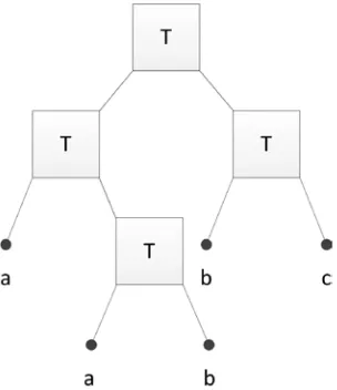
An introduction to the methods of decision tree classification is given in (Breiman et al., 1984); we state here the most important concepts. The principle of the decision tree classification is depicted in Figure 1. The set of data (root) is recursively split into two parts at nodes after a binary test (T). In its simplest form the test may be a threshold for an attribute of the data, e.g., the vegetation index. At each branch the remaining data are then tested at the next node down the tree. Here, the data are split again based on a binary test, e.g. by thresholding another attribute. The end nodes are the leaves of the tree. They represent the classes (categories). The threshold values can be found by expert knowledge (i.e. manually) or by supervised classification and statistical procedures. Pruning of the tree may also take place. The decision tree is derived from training data. For each class a number of points and their attributes are extracted. When the decision tree is derived, all data of the point cloud are classified, i.e. to each observation a class will be assigned. The noise in the training areas is important for the results and should therefore be checked.
Figure 1. Principle of decision tree classification. Modified after (Friedl and Brodley, 1997), where ‘T’ indicates a test and a,b,c the three possible classes
3. APPLIED METHODOLOGY IN THE GENERATION OF 2D LAND COVER MAPS IN URBAN AREAS
The applied methodology is based on a digital surface model (DSM), which is automatically derived from overlapping aerial images. Each DSM-point (-cell) with its spatial coordinates (Easting, Northing, and elevation) is supplemented by two attributes which characterize classes of land cover (vegetation index and height above ground). A decision tree classification is then used to assign a class to each point of the DSM. The decision tree is derived from training samples, which are collected by digitizing polygons on top of a false-colour orthoimage and extracting the points within the polygons. The generation of a land cover map needs some preparatory work, an assessment of the accuracy, and some refinements. All steps in the generation of a land cover map in urban areas will be described in the following sections. Figure 2 depicts the flowchart of the steps at the generation of a 2D land cover map.
Figure 2. Flowchart of the generation of a 2D land cover map
3.1 Preparatory work
The classes of the land cover map are in general specified with a specific application of the map in mind. Furthermore, the thematic accuracy is specified in advance either for each class (category) or overall. The producer of the land cover map has to select relevant data and methods in order to meet these specifications. Samples for training of the classifier and for assessment of the thematic accuracy have to be collected. The producer has to know, which features (attributes) characterize the individual classes, and which data can produce accurate and reliable results. Most important, the total costs of the production and of the assessment have to be within the agreements of the contract.
The applied method requires multispectral images with 60% forward overlap. The calibration parameters of the applied camera and the orientation parameters of all images have to be known. Such data may be derived by means of ground control and/or additional sensors at the camera. The preparatory work will then comprise the generation of a digital surface model (DSM) and an orthoimage. The derivation of the elevation model may use colour images. The orthoimage is compiled by
means of a false colour image and a digital terrain model (DTM). The DSM and the orthoimage are sources for the attributes of various land cover classes. In the proposed method the “elevations above ground” (dZ) and the “normalized difference vegetation index” (NDVI) are attributes which will characterize classes of vegetation and man-made constructions. The normalized DSM (nDSM) is obtained from the difference between the DSM and the DTM. The DSM is derived from two overlapping images by matching corresponding image parts and by interpolating a structured model of elevations. The DTM is obtained by filtering the DSM where buildings and vegetation above ground are removed. The elevations in both models are separated by a multiple of the ground sample distance (GSD). Nevertheless, the grid of elevations of both models is very dense. The accuracy of the derived elevations may become important for the result of the classification. Also the accuracy and resolution of the NDVI values will have an influence on the results.
3.2 Derivation of a decision tree
The proposed decision tree classification procedure requires the availability of a number of training areas for each class. These training areas are digitized as closed polygons on top of a false-colour orthoimage. At a position of a single DSM point the intensity values of the red and infrared channel of the orthoimage are extracted and converted into a NDVI value. A file with the spatial coordinates (E, N) and attribute values (dZ, NDVI) for each DSM point is created. By means of recursive partitioning of the training data set a decision tree is derived. It may be visualized as a plot of all nodes together with the calculated thresholds. In order to check for noise in the training areas all points of the training areas can be classified by using the derived decision tree. The accuracy of each class of the training data can then be assessed (cf. Section 3.4). If noise (misclassification) in the training data is absent, the thematic accuracy of each class will be 100%. This is, however, seldom the case.
3.3 Classification of all cells
The generation of the land cover map occurs by means of classification of all DSM cells and its attributes using the derived decision tree. Each DSM cell is assigned to a class. The result is plotted by means of coloured symbols. The number of cells belonging to one class can be calculated and used in sampling and weighting in the assessment of the overall accuracy.
3.4 Assessment
The assessment of the land cover map is done both visually and quantitatively.
3.4.1 Visual check
The derived land cover map should first of all be complete, which can be checked visually. Areas with no data may have occurred during the generation of the DSM. The gaps can only be closed by manual editing in combination with stereo observation of the images. Other refinements may also be required (cf. Section 3.5).
3.4.2 Quantitative assessment of the thematic accuracy The quantitative assessment of the thematic accuracy of the generated land cover map has to be based on sound statistical principles. An independent sample has to be taken and the
estimated accuracy measures of the sample are representative for the whole land cover map. The sample should have the proper size and the reference data should be of high accuracy and reliability. As the emphasis in this contribution is on the accuracy of the individual classes, a stratified simple random (STSI) sampling will be applied. This means that for each class a sample of predefined size is drawn by simple random sampling (without replacement). The number of sample units (observations) is calculated on the basis of the likelihood ratio test (LRT) confidence interval (Young and Smith, 2005). The reference values for cells can be determined by stereovision of false-colour image pairs. A Z-value of the sample unit is required for displaying the checkpoints in 3D. At such a position the ”true” class value of the point (cell) is found by the analyst. An error matrix can then be established from which the accuracy measures (overall accuracy, user accuracy, and kappa value) are derived. The stratified design has to be taken into account. Weights for each class are calculated by w=N/n, where ‘N’ is the number of cells in the land cover map and ‘n’ is the number of cells in the accuracy sample. The number of cells (or their area) are determined after the classification and calculation of the sample size.
3.5 Refinements
The produced land cover map may further be improved. The deficiencies of the ‘raw’ land cover map are gaps in the areas of the objects and misclassifications. Refinements have to be carried out with respect to applications (map updating or analysis) and the type of map (2D or 3D). With regard to map updating a high cartographic quality may be required. Buildings should be represented by straight and orthogonal lines. Solutions to this task are published by (Gross and Thoennessen, 2006) and (Sampath and Shan, 2007). The present article concentrates on the derivation and analysis of a land cover map. The ‘raw’ land cover map is converted into an image and the image map is then improved by the methods of image processing and image analysis. The necessary tasks are filling of gaps within the individual objects, derivation of outer boundaries, and removal of objects not belonging to one of the selected classes. These tasks can be carried out by filtering, morphological operations, and object manipulations.
4. APPLIED TOOLS
The imagery used in the practical example has been taken by the medium-format camera Leica RCD 30. The applied software tools include commercial packages, existing open source software, and newly developed programs. Details are given in the following sections.
4.1 Generation of DSM and nDSM
The generation and editing of the DSM as well as the generation of orthoimages are carried out by means of the software packages of the Trimble Company (“Match-T DSM”, “DTMaster”, and “OrthoMaster”). Numerous parameters have to be set in these programs which requires experience in order to obtain good results. In the generation of the DSM, e.g., the size of the search area for homologous points has to be specified. Filtering of the DSM needs to specify the spacing of an internal (less dense) elevation model and of cell heights in order to remove buildings and vegetation above ground. Details on these professional packages are contained in the manuals of
the producer. The normalized digital surface model (nDSM) has been derived by a program written in C++ language.
4.2 Classification and assessment
The classification and assessment have been carried out by newly developed programs using the open source language and environment “R” (R Development Core Team, 2013). Several R packages have to be used for this task. By means of the package “rpart” the decision tree is derived and by “ipred” (with function ‘predict’) the land cover map is generated. The packages “survey” (with functions ‘svydesign’, ‘svyciprop’, and ‘svykappa’), “binomSamSize”, and “binom” are used in the programs which derive the accuracy measures and its confidence intervals (Lumley, 2013; Höhle, 2009b).
4.3 Refinements
The derived land cover map has some problems regarding the lack of generalization and homogeneity of the areas representing the six classes. Errors in the classification have to be detected and removed. We propose to apply image processing techniques as implemented in, e.g., the R-package “EBImage” (Pau et al., 2013) in order to solve the mentioned tasks. “EBImage” is a toolkit for processing and analysis of images, which has been developed for microscopy imagery of biological content (cells). Applied functions are, e.g., ‘dilate’, ‘erode’, ‘fillHull’, ‘computeFeatures’, ‘makeBrush’. Various parameters have to be specified in these functions.
5. PRACTICAL TEST
In order to test the proposed method a 2D land cover map is generated and evaluated.
5.1 Description of test area and selected classes
The test area is an urban area in Switzerland of 1.4 ha. The 2D land cover map to be generated shall contain the six classes specified in Table 1, which also shows the discriminating features (attributes) to be used for the classification. The attributes (dZ, vegetation) of the classes vary considerably which is a prerequisite to assign each DSM cell to the proper class. The thresholds for the attributes will be determined by recursive partitioning of the training areas.
class dZ vegetation
building high none
hedge & bush low yes
grass none yes
road & parking lot none none
tree high yes
wall & car port low none
Table 1. Characteristics of the used land cover classes. (dZ=height of object above ground)
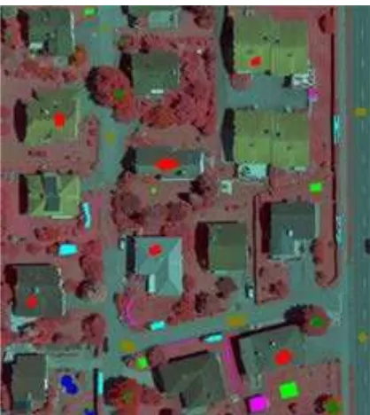
The test area contains some other categories, e.g., “swimming pool” and “field”. They will be classified into one of the six classes and thereby contribute to errors. Their area is, however, very small (cf. Figure 3). Objects like “hedge” and “wall” form very narrow lines which requires high-resolution imagery and accurate positioning when tracing the training areas.
Figure 3. Training areas on top of a false-colour orthoimage
5.2 Input Data
The multispectral images of the test area have a ground sampling distance of GSD=5 cm. Each pixel has four colours (red, green, blue, and near-infra red) with 256 intensity values each. The calibration data of the camera and the orientation data of the images were provided. The geometric quality of the camera and the used software package enable a high precision of the derived point cloud (σZ=0.04 m). The derived DSM and DTM have a spacing of 0.25 m. An orthoimage with a pixel size of 0.05 m is produced by means of the DTM and a false colour image. Six training areas for each class are digitized on top of the false-colour orthoimage (cf. Figure 3). Altogether, 17449 DSM-points were collected. The numbers per class (n) and the accuracy of each class are contained in Table 2. The accuracies of the classes are determined in the same way as the classes of the land cover map (cf. chapter 5.4). It is obvious from Table 2 that the accuracy of the class “wall and car port” is relatively poor (73%). The other classes have an thematic accuracy above 92% at the training areas.
class n accuracy
building 4204 100%
hedge & bush 3308 99%
grass 2680 93%
road & parking lot 3152 100%
tree 1829 92%
wall & car port 2276 73%
Table 2. Accuracies of classes derived from training areas
5.3 Processing of the land cover map
The processing starts with the derivation of the decision tree using the training areas of each class. The result is depicted in Figure 4.
Figure 4. Decision tree derived from training areas. (b=building, h=hedge & bush, g=grass, r=road & parking lot, t=tree, w=wall & car port, ndsm (dZ)=height above ground, ndvi=normalized difference vegetation index)
The decision tree has six intermediate nodes and seven end nodes. The automatically derived thresholds are written there. The leaves of the tree are marked with the abbreviations of the classes. Buildings, e.g., are classified when the height above ground is nDSM >= 4.47 m and the NDVI < -0.01555. By means of the derived decision tree the land cover map can be generated. For each point (cell) of the point cloud a class will be assigned.
5.4 Assessment of the produced land cover map
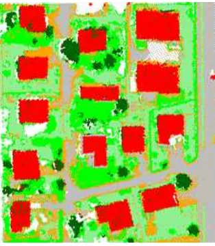
The visual inspection of the graphical representation of the derived land cover (cf. Figure 5) reveals a clear separation of the six classes. Buildings are very distinctly extracted despite the fact that the colours of the roofs are very heterogeneous in the false-colour orthoimage. Less visible are the walls, which are small in size and height. Many small cells, which represent the class “wall and car port”, appear in the classes “road” and “grass”. White areas are areas without data. Such gaps are the result of insufficient editing the DSM and are not corrected here. The generated land cover map is a ‘raw’ result, which can be improved by some refinements (cf. chapter 5.5).
Figure 5. Land cover map (‘raw’ result). Six classes are coded by colours. (red=“building”, light green=”grass”, dark green=”tree”, green=”hedge&bush”, grey=”road & parking lot”, orange=”wall & car port”)
The six classes are not equally distributed. The assessment of overall accuracy requires, therefore, appropriate weighting. The areas in per cent are 21% (“building”), 18% (“hedge and bush”), 25% (“grass”), 19% (“road and parking lot”), 4% (“tree”), and 13% (“wall and carport”). The size of the independent sample comprises 91 units (cells) for each class, i.e. 546 altogether. They are randomly extracted and their “true” class is found at their spatial position (E, N, Z) by stereo-observation in the oriented image pair of false-colour images. This approach leads to reliable reference values. The comparison between reference values and classified values is done by an error matrix (cf. Table 3). The classification result of the 91 units is written in rows separated for each class. In the diagonal of the matrix are the scores and outside the diagonal are the errors. The overall accuracy is calculated with 75% (95% CI: 72%-78%). When applying STSI weights the overall accuracy is 79% (95% CI: 76%-82%). The kappa value is 0.71 (95% CI: 0.66-0.75). According to (Landis and Koch, 1977) the derived kappa value of 0.71 represents a “moderate agreement” between the remotely sensed classification and the reference data. The survey weighted kappa is 0.74 (95% CI: 0.70-0.77) and thereby closer to “strong agreement” which starts with 0.80. The user’s accuracy of the individual classes and the corresponding 95% confidence intervals are contained in Table 4. Good results are obtained for the classes “building” and “road and parking lot” with 99% and 90% respectively. The poor results for class “wall and car port” (26%) was expected because noise in the training areas (accuracy=73%) has been monitored at this class (cf. Table 2).
5.5 Refinements
The refinement of the land cover map is carried out for each class separately. The class ‘building’ is used as an example. The application of the morphological operations (dilatation and erosion) improves the homogeneity of the buildings. The use of a “high-pass filter” derives the boundaries of all areas in class ‘building’. Some areas have to be removed. The connected sets of pixels (objects) are first labelled. Gaps inside the objects are then closed. Attributes of the objects (e.g., ‘size of area’, ‘centre of mass’) can be extracted for each object of the class.
Table 3. Error Matrix of the derived land cover map for the six classes. (b=”building”, h=”hedge&bush, g=”grass”, r=”road&parking lot”, t=”tree”, w=”wall&car port”)
class \
reference b h g r t w
row total
building 90 0 1 0 0 0 91
hedge &
bush 0 71 17 1 1 1 91
grass 3 8 74 5 0 1 91
road &
parking lot 5 2 0 82 1 1 91
tree 10 4 6 0 71 0 91
wall & car
port 8 8 8 43 0 24 91
column
total 116 93 106 131 73 27 546
Table 4. User’s accuracy of the derived classes
A threshold for the attribute ‘size of the area’ is used to remove objects not belonging to the class ‘building’. Figure 6 shows the result of the two steps of refinement. Other classes are handled in a similar way. The final land cover map is combined of all the refined classes. Classification errors may become visible and may be removed by means of other image processing.
Figure 6. Outer boundary of objects in the class “building” (left) and coloured objects belonging either to the classes “building” or “non-building” (right)
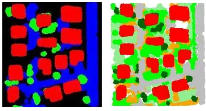
Figure 7 depicts two refined land cover maps. They are generalized and overlaps between the objects are removed.
Figure 7. Generalized land cover maps with three and six classes. The left map is produced by means of the red-, green-, and blue channel of the colour image, the right map is plotted using the same colours as in Figure 5
6. OTHER APPLICATIONS
The proposed method may use imagery of other sensors as well. The medium-format RCD 30 camera has recently be improved and may now be equipped with a 80 MP sensor (compared to 60 MP as in this investigation). The GSD will then be 1.15 times smaller when the images are taken from the same altitude. Images with four bands (red, green, blue, and near infrared) may also be taken by a large-frame camera which will reduce the amount of images necessary for a given area. Moreover, the
digital elevation models can be generated by means of airborne laser scanning or extracted from existing databases. The methodology to generate land cover maps can be the same as in this investigation. It is, however, of advantage when the necessary data are acquired by one sensor only and when they are collected at the same point of time. The urban areas may be very different too. The scenes may contain many other objects. The viewing angle and the ground resolution can also vary a lot. It is difficult to judge if the proposed method will work in all other scenes as well. Other testing has to follow.
Another practical test has, therefore, recently been carried out with building facades. In such an application the use of oblique aerial imagery is of advantage. Objects in the facades of buildings (windows, doors, walls, stonework, etc.) have to be detected, mapped and supplemented with information (position, dimensions, type of material, etc.). When determining four classes in the façades of a church (‘window’, ‘stone work’, ‘painted wall’, ‘vegetation’) by using intensities of oblique aerial images and elevations of these objects in a decision tree classification an overall accuracy of 80% has been achieved. The user accuracy of class ‘stonework’ and ‘window’ was assessed with 90% and 85% respecitively. The applied camera (RCD 30 Oblique) recorded three colour channels (red, green, blue) only. The results may be improved when multi-spectral oblique cameras are applied. The experiences with this example may indicate that the proposed methodology may also be successful in other scenes. In the two applications the object and image information are both used in the decion tree classification. The elevations have to be accurate and reliable. They may be derived from imagery only. This is a major characteristic of the applied methodology.
7. CONCLUSION
We propose a method to efficiently generate a large scale 2D land cover map from high-resolution imagery using decision tree classification. The obtained result for the overall accuracy of the derived land cover map with six classes (“building”, “hedge and bush”, “grass”, “road and parking lot”, “tree”, “wall and car port”) is 75% (95% CI: 72%-78%) and 79% (95% CI: 76%-82%) when weights for the size of classes are applied. The kappa value is 0.71 (95% CI: 0.66-0.75) and 0.74 (95% CI: 0.70-0.77) respectively. This is a moderate result (Landis and Koch, 1977). Strong results are obtained for the important classes “building” (99%), “road and parking lot” (90%), and grass (81%). Problems to overcome are the shadows of objects above ground, displacements of the objects in standard orthoimages and errors in filtering of the DSM. Improvements of the results are also expected when an average NDVI value is calculated for each DSM-cell so that the neighbourhood of a pixel is also included. The use of the decision tree classification of a point cloud with attributes “elevation above ground” and “vegetation index” is a very effective approach. Additional refinements by means of image processing techniques yield a generalized and homogeny land cover map.
The application of the R-packages for generation, assessment and refinement of land cover maps makes this approach easy to realize. The amount of work can be reduced when for the assessment of the thematic accuracy the cross validation is applied. The set of reference data is then used both for the derivation of the decision tree and for the assessment of the thematic accuracy. We preferred that the training areas and the test sample are completely separated from each other and that a
class accuracy 95% CI
building 99% 95%-100%
hedge & bush 78% 69%-86%
grass 81% 72%-89%
road & parking lot 90% 83%-95%
tree 78% 69%-86%
wall & car port 26% 18%-36%
relatively large amount of DSM points (here 17449 points=1.9% of all points) is used for the derivation of the decision tree.
In the presented investigations the imagery of a medium-format camera has been applied for a relatively small area. For large areas a high number of images has to be taken. Processing of a large amount of images is, however, no problem when distributed processing is applied. The proposed methodology has a high potential for automation and fast processing. The method has also successfully been tested with oblique images in order to detect and map objects of building façades and to extract information on these objects. The application of the proposed method to other urban areas and scenes seem to be possible. The event of new sensors and of advanced methods to extract elevations from imagery will support this view.
ACKNOWLEDGEMENT
The author thanks Leica Geosystems for providing image data and ground control points for these investigations. Michael Höhle, University of Stockholm, is thanked for support in programming and advices in statistical matters.
REFERENCES
Breiman, L., Friedman, J., Stone, C.J., Olshen, R.A., 1984. Classification and regression trees. CRC press
Foody, G.M., 2002. Status of land cover classification accuracy assessment. Remote Sensing of Environment 80 (1), pp. 185-201
Friedl, M.A., Brodley, C.E., 1997. Decision Tree Classification of Land Cover from Remotely Sensed Data. Remote Sensing of Environment 61, pp. 399-409
Giri, C.P. (ed.), 2012. Remote sensing of land use and land cover - principles and applications, CRC Press, Boca Raton
Gislason, P.O., Benediktsson, J.A., Sveinsson, J.R., 2006. Random forests for land cover classification. Pattern Recognition Letters 27 (4), pp. 294-300.
Gross, H., Thoennessen, U., 2006. Extraction of lines from laser point clouds, In: Symposium of ISPRS Commission III: Photogrammetric Computer Vision PCV06. International Archives of Photogrammetry, Remote Sensing and Spatial Information Sciences, pp. 86-91
Hansen, M., Dubayah, R., DeFries, R., 1996. Classification trees: an alternative to traditional land cover classifiers. International Journal of Remote Sensing 17 (5), pp. 1075-1081
Höhle, J., 2013a. Generation of Land Cover Maps Using High-Resolution Multispectral Aerial Cameras, In: GEOProcessing 2013: The Fifth International Conference on Advanced
Geographic Information Systems, Applications, and Services, IARIA, pp. 133-138
Höhle, M., 2013b. “binomSamSize: Confidence intervals and sample size determination for a binomial proportion under simple random sampling and pooled sampling”, R package version 0.1-3, 2013. http://cran.r-project.org/web/packages/binomSamSize/ (24 July 2014).
Höhle, J., Höhle, M., 2013. Generation and Assessment of Urban Land Cover Maps Using High-Resolution Multispectral Aerial Cameras. International Journal on Advances in Software, vol 6 no 3 & 4, 2013, pp. 272-282 http://www.iariajournals.org/software/ (24 July 2014)
Huang, C., Davis, L., Townshend, J., 2002. An assessment of support vector machines for land cover classification. International Journal of Remote Sensing 23 (4), pp. 725-749
Landis, J., Koch, G., 1977. The measurement of observer agreement for categorical data. Biometrics 33, pp. 159-174
Lumley, T. , 2013. R package "survey". http://cran.r-project.org/web/packages/survey/survey.pdf (24 July 2014)
Nex, F., Dalla Mura, M., Remondino, F., 2013. Integration of spectral information and photogrammetric DSM for urban areas classification. ISPRS Annals of Photogrammetry, Remote Sensing and Spatial Information Sciences 1 (3), 67-72.
Pau, G., Sklyar, O, and W. Huber, 2013. Introduction to EBImage - an image processing and analysis toolkit for R, http://www.bioconductor.org/packages/release/bioc/vignettes/E BImage/inst/doc/EBImage-introduction.pdf (24 July 2014)
Polikar, R., 2006. Ensemble based systems in decision making. Circuits and Systems Magazine, IEEE 6 (3), pp. 21-45
R Development Core Team, 2013. R: A language and environment for statistical computing, http://www.r-project.org (24 July 2014).
Sampath, A., Shan, J., 2007. Building boundary tracing and regularization from airborne LiDAR point clouds. Photogramm.Eng.Remote Sens. 73 (7), pp. 805-812
Thomas, N., Hendrix, C., Congalton, R.G., 2003. A comparison of urban mapping methods using high-resolution digital imagery. Photogramm. Eng. Remote Sens. 69 (9), pp. 963-972.
Young, G.A., Smith, R.L., 2005. Essentials of statistical inference, Cambridge University Press, Cambridge
Zebedin, L., Klaus, A., Gruber-Geymayer, B., Karner, K., 2006. Towards 3D map generation from digital aerial images. ISPRS Journal of Photogrammetry and Remote Sensing 60 (6), pp. 413-427