PHOTOGRAMMETRIC DETERMINATION OF DISCREPANCIES BETWEEN ACTUAL
AND PLANNED POSITION OF DENTAL IMPLANTS
G. Forlani a *, F. Rivara b
a
Dept. of Civil Engineering, University of Parma, Parco area delle Scienze 181/A, 43124 Parma, Italy- [email protected]
b Dept. S.Bi.BI.T, University of Parma, Via Gramsci 14, 43126 Parma, Italy
Commission V, WG V/1
KEY WORDS: Medicine, Photogrammetry, Close range, Measurement, Accuracy, Simulation
ABSTRACT:
The paper describes the design and testing of a photogrammetric measurement protocol set up to determine the discrepancies between the planned and actual position of computer-guided template-based dental implants. Two moulds with the implants positioned in pre- and post- intervention are produced and separately imaged with a highly redundant block of convergent images; the model with the implants is positioned on a steel frame with control points and with suitable targets attached. The theoretical accuracy of the system is better than 20 micrometers and 0.3-0.4° respectively for positions of implants and directions of implant axes. In order to compare positions and angles between the planned and actual position of an implant, coordinates and axes directions are brought to a common reference system with a Helmert transformation. A procedure for comparison of positions and directions to identify out-of-tolerance discrepancies is presented; a numerical simulation study shows the effectiveness of the procedure in identifying the implants with significant discrepancies between pre- and post- intervention.
* Corresponding author. This is useful to know for communication with the appropriate person in cases with more than one author. 1. INTRODUCTION
1.1 Motivations
Like many other disciplines, oral implantology exploits scientific and technological progress on material science and diagnostics. In the last years it has witnessed the application of new systems for treatment planning and surgical implementation based on computer tomography. Such systems allows for the transfer of a virtual CAD planning directly on the patient through surgical masks (see Figure 1) produced with CAM technology; the intraoral prosthesis is placed just after the insertion of the implant (see Figure 2) reducing the post-intervention times.
Figure 1. The surgical guide
However the clinical experience and several experimental studies (Valente et al, 2009; Schneider et al, 2009) have shown that small adjustment of the prosthetic are still necessary after
the operation, despite claims by the implant manufacturers that the error margin of the systems are negligible (Rinaldi and Mottola, 2010).
Figure 2. Dental implants
To test the validity of these surgical guides, in most cases the position of the implants in Computer Tomography images before and after the surgery is compared with matching techniques (Maes et al, 1997; Wanschitz et al, 2002) based on mutual information theory (Papoulis, 1991; Woods, 1992), a similarity measure often used in medical imaging. In other cases ad-hoc radiographic markers are placed to help in the registration of the two sets of pre- and post-intervention images (Widmann et al, 2010), for instance by inserting in the bone tissue a few screws acting as stable reference (Holst et al, 2007). In other cases, when studying the performance of assisted implantology (Brief, 2005) a direct comparison with a Coordinate Measuring Machine has been performed on the models and their copies taken from impression of the patient mouth.
To evaluate the accuracy of implant insertion by photogrammetry, the Department of Civil Engineering and the
Dentistry Section of the Dept. S.Bi.BI.T of the University of Parma joined in cooperation. Compared to the above mentioned techniques, photogrammetry offers three advantages:
- no further radiographic imaging are necessary, after those for planning the treatment
- optical images do not suffer from blooming effects (voxel) resolution of about 25 micrometres.
1.2 Parameters used to compare master and copy
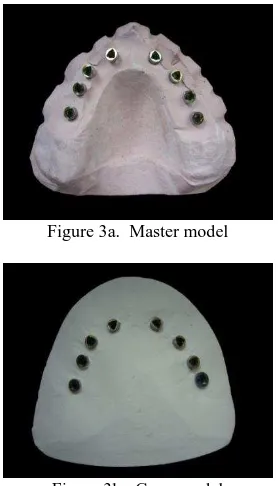
To evaluate metrically by photogrammetry the differences between the planning designed with the help of CT images and implemented in the surgical mask and the actual placement realized on the patient, two moulds (models) each carrying the implants are compared (see Figures 3a and 3b). The former is obtained directly from the surgical mask (master model), inserting the implants in the guides and then by enclosing them in a gypsum mould; the latter is produced from the dental impression of the patient and therefore shows the actual position of the implants after the surgery (copy model).
Figure 3a. Master model
Figure 3b. Copy model
To compare the two models and evaluate the discrepancies in the implant position, different parameters can be taken into account. In the literature on this topic, most authors use the four parameters shown in Figure 4. The implant’s head of the master model is the reference point; the implant’s symmetry axis of the master model is the reference axis. The discrepancies between the positions of the two heads and the two apices of the implant are expressed in two components: along the reference axis and perpendicular to it; moreover, the angle between the reference axis and the implant axis in the copy model should be determined.
Unlike TC imaging, a direct measurement of the discrepancy at the apex of the implant by photogrammetry is obviously impossible. If the implant can be considered rigid enough, (so
that no shape deformation occurs), it is possible to compute the discrepancy from the other parameters.
Figure 4. Parameters used to describe the differences between the master and the copy model
The paper is organized as follows: Section 2 describes and discuss how the geometric parameters of Figure 4 can be recovered from photogrammetric measurements, referring them to the same coordinate system; Section 3 illustrates the design and implementation of a photogrammetric measurement protocol; finally, Section 4 describes the simulated and experimental results to test the system and its capability to identify out-of-tolerance discrepancies between the planned and actual implant positions.
2. DETERMINATION OF THE PARAMETERS FOR
THE COMPARISON OF MASTER AND COPY
2.1 Computation of the discrepancy parameters
Let M and C be the locations of the master and copy heads; let
c
be a parametric representation of the implant axis in vector and scalar notation, where:
where ““ and “ “ are the dot and vector product symbols respectively. The angle between the implants axes can be computed from the dot product of the unit vector of the two axes:
(3)
For the above operations to be meaningful, the head’s locations and the axes directions must be expressed in the same reference system. Indeed, this is the main difficulty in comparing master and copy, for theoretical as well as practical reasons.
2.2 Referring implants positions and inclinations to the same coordinate system
As can be seen from Figure 3, the master and copy model have very few features in common, that might be used as homologous points in a reference system transformation. It would be better to include some details of the patient mouth with defined features; in practice, only the gums might be used. If a very detailed survey could be produced (e.g. using a very accurate triangulation system, such as in Ettl et al, 2010) the two models might then be aligned with a surface matching method like the Iterative Closest Point (ICP, Besl & McKay, 1992) without using information from the implants. This method has actually been tried with triangulation systems with mixed results; it has also the drawback of lacking information on the quality of registration and its influence on the parameters to compute. Using photogrammetry, the survey of master and copy will be carried out in two distinct reference systems and therefore it is necessary to find homologous (i.e. unchanged) elements in both systems to compute a Helmert transformation. Looking again at Figure 3 the only possibility is to use the implants themselves as common points. But the goal being to find out whether they have changed or not, two questions arise:
1. systematic discrepancies between master and copy that will be absorbed by the Helmert transformation Helmert transformation will treat such inconsistencies as due to random errors to be minimized; this will bias the estimates of the parameters of Figure 4.
It is therefore necessary to study when the Helmert parameters discrepancies exceeding the tolerance. In Section 4 these problems will be addressed by simulations with synthetic data. Moreover, in order to compute the geometric parameters of Figure 4 it is necessary to attach targets to the implants in the two models, determine their coordinates photogrammetrically, derive the position and orientation of the implants axes of both models and then transform those of the copy model into the master model. As far as the transformation of the heads of the implants is concerned, a Helmert transformation is used:
z
X, Y, Z = coordinates of a point in the master system x, y, z = coordinates of a point in the copy system X0,Y0,Z0 = shift parameters
R = rotation matrix from copy to master system s = scale parameter
copy system and in the master system respectively
Given two sets of nominally identical points in both reference systems, the transformation parameters can be estimated with an over determined equation system. If a significant percentage of outliers (i.e. possibly false correspondences or gross errors in the measurements) is expected, a robust estimation method should be used; in case of normally distributed errors, the Least Squares Estimation (LSE) method in widely used since it has the additional advantage that confidence regions for the estimated values can be derived and parametric hypothesis testing on measurement errors values can be performed (Kraus, 1997). The least squares method also provides a framework for the mathematical definition of concepts like measurement reliability and minimum detectable error, useful to assess the quality of the measurement system; the accuracy and the determinability of the parameters can be studied as a function of the number and distribution of identical points on the object. Actually, the determinability of the transformation parameters is one of the critical issues in this specific context; there is little freedom in selecting or placing identical points on the master and the copy: only the implants can be “safely” used to this end. Therefore in principle at least three implants are necessary to compare a master and a copy; however, near-degenerate configurations might arise that prevent the (correct) estimation of some parameters: think for instance of a few implants (3-4) almost aligned on a straight line: in this case the rotation around that straight line cannot be determined. However, if the measurement method provides also the axes directions, this information can be added to the estimation process, reducing the number of points and directions necessary.
2.3 Evaluation of deviations based on geometric invariants
As pointed out in the previous paragraph, a comparison of the implants based on coordinates in the same reference system has some drawbacks. Alternatively, inconsistencies between master and copy can also be highlighted by computing or measuring geometric properties, such as distances between implant heads and angles between implants of the same model, that are invariant with respect to the reference system (the latter is also scale independent). Since distances involve pairs of points and angles involve groups of three points, only relative changes can be highlighted (i.e. you cannot tell whether both or just one of the implants has changed position with respect to the master)
four parameters of Figure 4 can still be computed (though in a less straightforward way).
3. PHOTOGRAMMETRIC MEASUREMENT
PROCEDURE
3.1 System design and preliminary trials
Since an extended series of data must be collected to reach statistically sound conclusion on the actual quality of the guided implantology, a measurement protocol has been established that might be carried out also by a non-photogrammetrist.
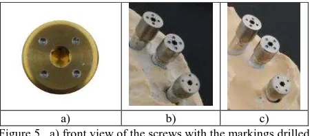
From a literature survey on the topic, an accuracy better than 0.1 mm on the position and better than 1° has been set as goal. The models have dimensions of about 7 cm by 7 cm and a height between 3 and 4 cm. The implant head diameter varies from 3.5 mm to 5 mm. Apart from network design, the major difficulty is how to mark or place on the implant a point representative of the head location and how to compute the inclination of the implant. As far as the former goal is concerned, the obvious choice would be the center of the implant head, i.e. a point on the axis of symmetry of the implant. Since the implant is hollow, either the center of a screw head must be used or it might be computed as center of points, placed on the screw head symmetrically with respect to the implant axis. Moreover, since the accuracy of the collimation influences the accuracy of the point determination, the physical mark representing the point must have good contrast and appropriate size for the collimation; moreover, his thickness should be negligible with respect to the accuracy required. In the case of the Nobel implants, the screw provided by the same manufacturer was used, since they fit perfectly to the implant axis. Using a numerically controlled machine (NCM), four circular holes 0.5 mm large were drilled on each screw (Fig. 5), at the corner of a square whose centre coincides with the implant axis within 0.02 mm. Notice that the center hole of the screw cannot be used because it’s too large for an accurate collimation; moreover, to provide information about the implant axis direction, more than one point is necessary. The same screw was used for both implants in the same position of the master and copy, to account for small possible differences; the position of a given mark on a screw is not exactly the same on the master and the copy, though: looking at Figure 4b) and 4c) it can be noticed that while the marks on the upper left screw pair look in identical position, a rotation is apparent between the four marks of the two other screws. This means that while the implant head position will be the same, the marks on the screw cannot be used directly in the Helmert transformation, because they are not truly homologous points.
a) b) c)
Figure 5. a) front view of the screws with the markings drilled by a numerically controlled machine; b) and c): the same three screw mounted first on the copy and then on the master (c).
Notice that the same marking is not in the same position
Since the size of the model is rather small, it can be imaged in a single image; this suggests using a convergent imaging
geometry at the largest feasible image scale, i.e. getting as close as possible to the object, in order to fill the whole image format. This has to be balanced with the depth of field necessary to maintain sufficient image sharpness: the more inclined is the camera axis with respect to the normal to the object, the larger the depth of field required and the perspective deformations of the marks.
To ensure a common scale factor for all models and a stable block orientation, a reference frame was set up on a steel plate; known object points were provided by drilling 16 holes on the plate (see Fig. 6) with the same numerically controlled machine used for the screw. The holes are placed on a circumference of 120 mm, with a constant angular spacing. Although remarkable, in this case the accuracy of the known points is comparable to the theoretical accuracy of the photogrammetric point determination (more on this point later): in principle therefore the block adjustment should consider also the “known” point coordinates as random variables and the empirical accuracy evaluation based on check points should also take this into account.
The plate has in its lower face a ring that fits into a cylindrical base; this is used to rotate the object in regular angular steps, while the camera remain fixed on a tripod; this speeds up image acquisition and maintains a constant average image scale. Although they provide an effective way to control the photogrammetric block, the holes in the plate are not ideal targets. Indeed, when seen from nadir and with illumination direction almost horizontal, they appear as regular black dots against the background, i.e. almost ideal to collimate.
Figure 6. The steel plate with the 16 holes drilled by the numerically controlled machine and a master with the screws inserted in the 6 implants
Unfortunately, the imaging direction is not from nadir because convergent images are necessary to try to get homogeneous accuracy in the three coordinates; moreover lighting must ensure that also the model is properly illuminated, so light will be diffuse and coming from several sources. Therefore, depending on the illumination direction and intensity, on the depth of the hole, on the reflections from the polished inner surface of the hole, its shape and contrast might change from image to image. Rather than a real mark (i.e. a well defined point on a flat surface) what is actually being collimated is a hole. This makes it difficult to precisely and consistently identify the same point: in fact, rather than the center of the hole at the plate level, a point along the axis of the hole, perhaps a slightly different one from each image will be actually collimated. This uncertainty in the definition of the point demands for an additional measurement effort: using many images from different directions should mitigate and at least partially compensate such problems; careful setting of the
illumination and of the camera axis inclination is very important.
Collimation of points on metallic surfaces from different directions is always going to be difficult because the light reflections can vary the object sharpness and contrast dramatically. Since images are taken all around the object, the light should be as much as possible diffuse; direct reflections towards the camera should also be avoided, therefore the lamps position (elevation above the plate plane) is to be checked. To this aim, the plate with the model is inserted in a specially designed soft box. Although not wholly symmetric, the illumination obtained is diffuse enough to avoid reflection spots on the images. A disadvantage of this solution is that the illumination will slightly change from image to image due to the rotation of the plate; in principle a solution with the illumination sources fixed with respect to the object (i.e. to the plate) would be better.
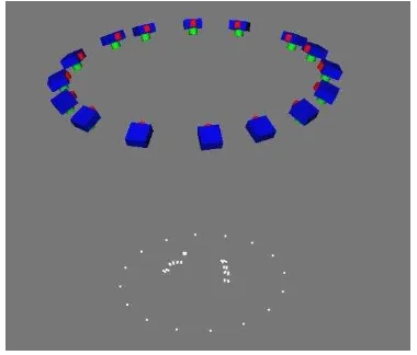
Figure 7. The photogrammetric network: 16 camera stations, the object control points on the plate and a model with 8 implants
A first series of tests has been carried out with a Nikon D100 (6 Mpix, image format of about 23x15.6 mm) with 18 mm and 50 mm lenses; after some trials with stations including either convergent and nadir images, a single ring of 16 convergent images was found to be the best compromise between precision and number of images (see Figure 7).
Using the shortest focal length at the minimum focussing distance with sufficient depth of field only about half of the format is filled; using the 50 mm lens, the minimum focusing distance increases, but there is a better filling of the image format: the overall accuracy of the point determination from the Bundle Block Adjustment (BBA) is slightly better (see Table 1). Finally, a Nikon D3x has been made available, together with a 35 mm lens. The Nikon D3x has a resolution of 6500x3800 pixels and full frame format of 36x24 mm; with the 35 mm lens a better combination of image scale, image format filling and pixel resolution on the object was obtained; this is reflected in an overall dramatic improvement in the estimated precision.
RMS() from BBA X (m) Y (m) Z (m) Nikon D100 – 18 mm 18 18 24 Nikon D100 – 50 mm 15 15 20
Nikon D3x – 35 mm 4 4 7
Table 1 – Precision estimates from the BBA: RMS of the coordinate’s standard deviations of the points on the implants, with different combination camera-lens; results refer to a block with 16 images and camera focused at the shortest distance.
3.2 Measurement of the available set of models
After establishing the measurement protocol, all the 11 model pairs available for the testing of the photogrammetric procedure, each with a number of implants varying from 3 to 8, have been measured.
For the image acquisition, the camera is mounted on a tripod and set in such a way that its axis points towards the steel plate centre; the inclination of the camera axis with respect to the normal to the plate is 25° and the distance of the camera from the object is set to 25 cm (the minimum focusing distance); this ensures the largest image scale with a still sufficient depth-of-field. The model with a screw in each implant is placed at the centre of the plate; in the survey of the model copy, the same screw will be screwed to the corresponding implant of the copy. A total of 16 images are taken, evenly spaced angularly, by rotating the plate.
The image coordinates of every control point on the plate and every mark on a screw are manually collimated in every image; in case of a model with 8 implants, this means a total 16*(8*4+16) = 768 collimations. With some practice and using efficiently the software tools to speed up the collimations, an 8-implants model can be measured in about 1h 30’ by a non-photogrammetric.
The precision estimated by the bundle adjustment for the markers on the screws is about 4 m in X and Y (the steel plate plane) and 7 m in Z; because of the symmetry, such values are practically constant all over the object. The same values have been consistently obtained in all measured models (105 implants on 11 pairs master-copy). Being the measurement area about 12 cm by 12 cm, the relative accuracy in XY is about 1:30.000, half so in Z. The asymmetry in precision between XY and Z cannot easily be improved, though, because of the limited depth of field. The former is more important in the estimation of the implant position while Z determines the inclination of the implant. By using only 8 equally spaced images, the precision gets worse by 50%, though the coordinates change slightly only in Z.
3.3 Computation of the geometric parameters
The results of the photogrammetric measurements provide the input data for the estimation of implants heads and axis direction, performed with a Matlab script. For every model and copy pair, using clustering techniques, the four marks on each screw are identified in the exported adjusted coordinates. For each screw, the average position of the marks is computed. The direction of the implant axis is estimated as the unit vector n
normal to the LSE best fit plane of the four marks. In both cases, the redundancy of measurement allow to fix empirical thresholds to prevent biases in the estimation due to (unlikely) gross errors possibly affecting the adjusted coordinates of one of the marks: this is obtained by comparing, on each screw, the normal direction to the plane defined by using three marks at a time and by comparing the distance of opposite marks pairs. Next, the homologous screws of the master and copy are automatically paired to compute the Helmert transformation; since the information on the normal would otherwise not be used and this may lead to numerical instability (see Section 2.2), another homologous point is “artificially” introduced along the axis of each implant. This point incorporates the information on the normal direction coming from the measurement of the four marks; the point is generated at a distance from the implant’s head where the uncertainty of the axis direction matches the XY uncertainty of the implant head.
After the computation of the Helmert transformation and the evaluation of the results, the geometric parameters of Figure 4 are computed for each implant in each model. Moreover, also a matrix with the inter-distances between each implant in the model and a matrix with the angles between the axes of each implant pair in the model are computed for the master as well as the copy.
Finally, a classification of the discrepancies found in each model pair is performed (see next section) to accumulate data for the evaluation of the guided implantology accuracy.
4. EMPIRICAL TESTS AND SIMULATIONS TO ASSESS THE SYSTEM DISCRIMINATION
CAPABILITIES
4.1 System accuracy and repeatability with real data
A series of empirical and numerical tests have been performed to assess the performance of the procedure and of the measurement protocol.
The same master model with 8 implants has been measured photogrammetrically twice using the steel plate as reference. In both cases the estimated precision of every mark from the bundle block adjustment turned out to be about 4 m in XY and about 7 m in Z. In order to have an independent assessment of this estimated accuracy, the bundle block was oriented by fixing the coordinates of just 8 of the 16 marks. The remaining 8 marks were treated as check points. The Root Mean Square (RMS) of the differences turned out to be 10 m in XY and 20
m in Z, with no systematic components.
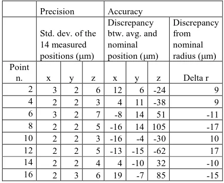
Moreover, for 7 master-copy pairs, the block has been also adjusted using only 8 control points (every other one of the 16) and the remaining 8 as check points. Table 2 provides the statistics of the differences for the 8 points over the 14 models.
Precision Accuracy
Table 2 – Bias in the estimates of the geometric parameters due to random errors, obtained by synthetically generated data
In the columns under “Precision” the standard deviations in m of the 14 coordinates of the same point are reported. This is a measure of the repeatability of the measurement protocol. Under “Accuracy” the difference between the average of the 14 coordinates and the nominal value of the coordinate is reported. This is a measure of the average accuracy of the measurement protocol. Notice that for the Z coordinate there is no reference nominal value from the plate manufacturer, so a flat plate has
been considered. In the last column the difference with respect to the nominal radius are reported.
Taking into account that the nominal accuracy of the reference XY coordinates is 20 m and the standard deviations of the measured positions, not only the average accuracy but also each coordinate is almost always within tolerance (i.e. within 20 m from the nominal value). The discrepancies with respect to. the nominal radius of the circle where the holes were made show some systematic behaviour, since in two opposite quarters of the plate they turn out to be compressed and stretched in the other two.
To assess the repeatability of the measurements with respect to the determination of the geometric parameters, the midpoint of the line segment connecting opposite marks is computed and the discrepancy between the two positions has been evaluated; the average distance between the midpoints of the line segment connecting opposite marks of the screw turned out to be 10 m. The direction of the implant axis is estimated as the unit vector normal to the LSE best fit plane of the four marks. To assess the quality of the axis direction estimation, the unit vector is also computed for all 4 combinations of groups of three points and the angle with respect to the over determined solution computed. The RMS value of the differences turned out to be 0.3°, but with largest values close to 1°.
4.2 Numerical simulations to assess system discrimination
Though the empirical results show system accuracy within the specifications, it is important to find out the system capability to actually identify discrepancies between the position and inclinations of implants under realistic conditions. This implies that, without implants actually changed, the actual bias on the parameters of Figure 4 is negligible under random measurement errors. The second is to show that, when measurement errors and truly changed implants are present, there is an effective procedure to identify such implants.
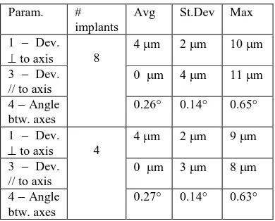
In both cases, a series of numerical simulations has been performed based on synthetically generated data. A master model was generated by simply taking the implant head positions of a real master model as true values; then, error free positions of the 4 marks were computed for each screw; with a known Helmert transformation applied to the marks, an error free copy model was generated in a different reference system. Finally, the coordinates of the marks in both models were corrupted with normally distributed errors with zero mean and standard deviation of 4 m for the XY coordinates and 7 m for the Z coordinates. A total of 90 synthetic master-copy pairs with different randomly generated errors were processed, to build a statistic on the estimation errors of the deviation parameters. Table 3 summarizes the results of the numerical tests with reference to the classification of the deviations of Section 2.2. Two models were processed: with 8 implants (4 on the left side and 4 on the right) and with 4 implants (all on the same side, a case with potential numerical instability in the Helmert transformation). For each model, the average, the standard average bias (if any) that the photogrammetric measurement process and the Helmert transformation introduces on the estimation of the deviations (or, in other words, the accuracy of the evaluation of the deviations). As far as the deviations
perpendicular to the axis are concerned, the average is consistent with the 4 m error introduced; since this deviation is in fact a distance, no averaging is possible; the deviation parallel to the axis, being a signed quantity, has an average of 0
m. The angle between axes, a positive quantity, is slightly
Table 3 – Bias in the estimates of the geometric parameters due to random errors, obtained by synthetically generated data
As it is apparent from the table, there is no difference between the 8-implants case and the 4-implants case and the bias on the estimates is small enough compare to the tolerances set for the system.
In order to verify the capability of the method to identify true differences between the master and copy, a series of simulations have been performed, introducing random measurement errors and gross errors (i.e. true changes between master and copy) in the coordinates of the copy model. The zero-mean random errors on the XYZ coordinates of the markings have standard deviation of 4 and 7 m respectively for XY and Z coordinates; the gross error representing the change in inclination of an implant is generated by a rotation of the implant that affects the coordinates of its four markers. The gross error is about 4 times the estimated parameter precision.
More specifically, in the case of the 8-implants model and error of 1° has been introduced in 4 combinations: 1, 3, 6 and all and copy larger than 3 times the estimated precision; 2) a value exceeding 1.5 of the ratio between the average
variation of inclination of the implant with respect to all other implants and the the average value of such variation for all implants;
3) a value of the average variation of inclination larger than 3 times the estimated precision
A total of 100 simulations (each involving an 8-implants master and copy) have been run for each error combination mentioned above. The results are summarized in Table 4, where a classification matrix is used to assess the success rate and the failure to identify the error.
1 implant changed in each copy model Implants 3 implants changed in each copy model
Implants 6 implants changed in each copy model
Implants 8 implants changed in each copy model
Implants identification of changed implants between master and copy.
As could be expected, the capability of the system to find outliers (i.e. actually changed implants inclination) decreases with the increase in the number of changed implants from above 99 % to about 88%.
5. CONCLUSIONS
A photogrammetric procedure to measure the discrepancies between the planned position of oral implants and their actual position after surgery has been presented. The measurement protocol and the setup (sample preparation, image acquisition and measurement) though not trivial, are simple enough to be used after a small amount of training. Improvements could be made if the markers on the screw and the reference plate could be marked with a better accuracy. The procedure, unlike other techniques presented in the literature, is able to provide estimates of the accuracy of the result, which appear to be consistent with the system requirements. Overall, the influence of random measurement errors on the estimated direction of the implant axis is less than 1° and is negligible for the position of the apex.
Empirical thresholds have been defined to label as changed or unchanged the position and inclination of an implant. The capability to successfully identify true differences between the planned and actual position has been tested numerically by
actually changing 1, 3 or 6 implants in the case of 8 implants. Based on a error classification matrix, this capability it turns out to be very satisfactory, though obviously decreasing with the number of really changed implants. More testing is needed for cases with a smaller number of implants where the discrimination capability might be more limited.
In the meantime the system has already being used with real data from 11 patients; this is part of the next phase of the research and results will be reported in a future paper, as soon as a statistically significant amount of data is collected.
6. REFERENCES
Besl, P. J., McKay, N. D., 1992. A method for registration of 3-d shapes. IEEE Trans. Pat. Anal. an3-d Mach. Intel. 14(2), Feb 1992, pp. 239-256.
Brief, J., et al., 2005. Accuracy of image-guided implantology.
Clin Oral Implants Res, 2005. 16(4): p. 495-501.
Ettl, S., Arold, O., Willomitzer, F., Yang, Z., Häusler, G., 2010. “Flying Triangulation“ – Acquiring the 360° Topography of the Human Body on the Fly. Proc. of the 1st Int. Conf. on 3D Body Scanning Technologies, Lugano, 19-20 october 2010. N. D’Apuzzo ed., ISBN 978-3-033-02714-5, pp.
Holst, S., Blatz, M.B., Eitner, S., 2007. Precision for computer-guided implant placement: using 3D planning software and fixed intraoral reference points. J Oral Maxillofac Surg, 65 (2007), pp. 393–399.
Koong, B., 2010. Cone beam imaging: is the ultimate imaging modality? Clinical Oral Implants Res., 2009. Vol. 21/2010, pp. 1201-1208.
Kraus, K., 1997. Photogrammetry. Volume 2: Advanced Methods and Applications. Ferd-Dümmlers Verlag
Maes, F., et al., 1997. Multimodality image registration by maximization of mutual information. IEEE Trans Med Imaging, 1997. 16(2): p. 187-198.
Papoulis, A., 1991. Probability, Random Variables, and Stochastic Processes. McGraw-Hill, Inc.
Rinaldi, M., Mottola, A., 2009. Superamento degli ostacoli anatomici in chirurgia implantare - Implantologia computer-guidata - Innesti ossei. Elsevier - Masson, Milan, 460 pp.
Schneider, D., Marquardt P., Zwahlen M., Jung R.E., 2009. A systematic review on the accuracy and the clinical outcome of computer-guided template-based implant dentistry. Clinical Oral Implants Res., 2009. Vol. 20 Suppl 4: pp. 73-86.
Valente F., Schiroli, G., Sbrenna, A., 2009. Accuracy of computer-aided oral implant surgery: a clinical and radiographic study. Int. J. Oral Maxillofac. Implants. 2009 Mar-Apr, 24(2); 234-242.
Wanschitz, F., et al., 2002. Evaluation of accuracy of computer-aided intraoperative positioning of endosseous oral implants in the edentulous mandible.Clin Oral Implants Res, 2002. 13(1): p. 59-64
Widmann, G., et al., 2010. Comparison of the accuracy of invasive and noninvasive registration methods for image-guided
oral implant surgery. Int. J. Oral Maxillofac. Implants. 2010. 25(3): p. 491-498.
Woods, R.P., Cherry, S.R., Mazziotta, J.C., 1992. Rapid automated algorithm for aligning and reslicing PET images. Journal of Computer Assisted Tomography 16(4): 620–633.