PHOTOGRAMMETRIC PROCESSING OF HEXAGON STEREO DATA FOR
CHANGE DETECTION STUDIES
E. Anantha Padmanabha*, P. Shashivardhan Reddy, B. Narender, S. Muralikrishnan, V. K. Dadhwal.
(National Remote Sensing Centre – Indian Space Research Organization, Hyderabad-37, India)
(anantha_p, shashivardhan_r, naren_br, muralikrishnan_s,)@nrsc.gov.in, [email protected].
Commission VIII, mid-term symposium 2014
KEY WORDS: Corona, Hexagon, Cartosat-1, RSM, RFM, change detection
ABSTRACT:
Hexagon satellite data acquired as a part of USA Corona program has been declassified and is accessible to general public. This image data was acquired in high resolution much before the launch of civilian satellites. However the non availability of interior and exterior orientation parameters is the main bottle neck in photogrammetric processing of this data. In the present study, an attempt was made to orient and adjust Hexagon stereo pair through Rigorous Sensor Model (RSM) and Rational Function Models (RFM). The study area is part of Western Ghats in India. For rigorous sensor modelling an arbitrary camera file is generated based on the information available in the literature and few assumptions. A terrain dependent RFM was generated for the stereo data using Cartosat-1 reference data. The model accuracy achieved for both RSM and RFM was better than one pixel. DEM and orthoimage were generated with a spacing of 50 m and Ground Sampling Distance (GSD) of 6 m to carry out the change detection with a special emphasis on water bodies with reference to recent Cartosat-1 data. About 72 new water bodies covering an area of 2300 hectares (23 sq. km) were identified in Cartosat-1 orthoimage that were not present in Hexagon data. The image data from various Corona programs like Hexagon provide a rich source of information for temporal studies. However photogrammetric processing of the data is a bit tedious due to lack of information about internal sensor geometry.
1. INTRODUCTION
Change detection is the process of ascertaining specific changes among the features of interest within certain period of time. Change detection analysis of spatial features is an important process in understanding the growth patterns and for planning the future development of rural and urban areas of a developing nation. Remote sensing technology has been effectively used in the recent past for change detection analysis for various projects in India. The process requires spatial information of the area of interest for different periods of time. The temporal resolution depends on the availability of the archival data for different time periods. A very high temporal resolution may lead to redundant information and may also put unnecessary load on the processing system. Presently there are many remote sensing satellites acquiring data with various spatial and spectral resolutions. At present the temporal frequency of remote sensing data from various sensors is high and automation in processing is possible as the data is in digital format (Hussain et al., 2013). The main problem is the availability of historical data for the area of interest and acquired at the desired point of time. If the data sets are available with required specifications as per the project demand, remote sensing technology can do wonders in detecting even the subtle changes both in terms of quality and quantity. Remote sensing data acquired at regular intervals of time can provide a better understanding of the characteristics and distribution of the changes either natural or manmade (Shaoqing and Lu, 2008). This helps administrators and policy makers in monitoring the change for future planning and making better decisions. In view of these merits, the remote sensing technology has been widely accepted for change detection analysis of both rural and urban areas for planning and development.
* Corresponding author.
The first remote sensing satellite Landsat-1 (80 m GSD) was launched in 1972 by NASA followed by a series of Landsat satellites. First high spatial resolution, remote sensing satellite was launched in 1986 by SPOT with a GSD of 10 m (Campbell and Wyne, 2011). Indian Space Research Organization (ISRO) launched its fist operational remote sensing satellite IRS-1A in 1988 followed by IRS-1B and IRS-1C (Kasturi Rangan et al., 1996). Subsequently ISRO launched a series of remote sensing satellites viz. Oceansat, Resourcesat, Cartosat etc. Presently ISRO has a fleet of remote sensing satellites with various spatial resolutions and spectral bands (Navalgund et al., 2007; www.isro.org). It is very important to acquire and store data from all the possible satellite missions so that this becomes a rich source of information for future studies and analysis. Earlier this was a costly affair due to the limitations of onboard storage, data reception and storage systems. Now with the advancements in the technology, the data reception and storage capability has improved and available at a reasonable cost. Till the declassification of data acquired through Corona program, change detection was limited to the last couple of decades and for only selected areas. Now there is a huge archival of data for change detection studies which aids in modelling various natural or human induced spatial phenomena (Jianya et al., 2008).
1.1 Corona Program
Corona was a photoreconnaissance satellite program jointly launched, operated and managed by Central Intelligence Agency (CIA) and United States Air Force. This program includes a number of satellites with onboard film cameras, recovery vehicles to collect the exposed film from mid air. The cameras and the films used have undergone much technological advancement as the program spanned for over two decades. The main objective of this program was to acquire photographic intelligence regarding the arms proliferation from different parts ISPRS Annals of the Photogrammetry, Remote Sensing and Spatial Information Sciences, Volume II-8, 2014
of the world primarily from communist controlled nations like USSR and China (Anderson, 2005). This data was acquired during the cold war period, post the World War II for over two decades in 60s and 70s. The satellites launched in this program were designated as KH1, KH2, KH3 and KH4 where KH stands for Key Hole. As part of this program many satellite missions were launched with code names Argon, Lanyard, Gambit, Hexagon etc. Initially this data was classified and had restricted access to the authorized defence personnel. Hence the civilian community was not even aware of its existence. Some of the data acquired through this program was declassified partly in 1995 and 2002 in phases. (Dashora et al., 2007; Surazakov and Aizen, 2010).
1.2 Hexagon Satellite
After the initial success of Corona program, United States felt the need to improve the capabilities of photo reconnaissance with larger coverage and better spatial resolution. As part of this, a series of 20 satellite missions with increased spatial resolutions were launched with the code name Hexagon KH9. This program was launched in 1971 and was in action for acquiring photographic images till 1986. There were two camera types onboard Hexagon, a twin panoramic camera with 2-3 feet spatial resolution and a frame type mapping camera with 30-35 feet spatial resolution. Subsequently the spatial resolution was increased to 2 feet and 20 feet respectively. About 29000 photographs were captured through this mission covering most of the world except few regions like Antarctica, Greenland and Australia. Most of these images were declassified in 2002 by US government for civilian use (NRO, 2011; Surazakov and Aizen, 2010). Image data acquired as part of these photoreconnaissance missions like Corona and Hexagon contribute significantly to the change detection studies (Narama et al., 2010). These data sets significantly improve the limited archival data available for temporal studies as they were acquired long before the launch of the first civilian remote sensing satellite i.e., Landsat-1 in 1972. The data is available for many parts of the world in high resolution at an affordable cost (Dashora et al., 2006; Surazakov and Aizen, 2010).
2. SENSOR MODELING
A sensor model defines the mathematical relationship between 2D image coordinates and the 3D object coordinates (Hu et al., 2004). In photogrammetry orientation of a stereo pair of images can be done either using a rigorous sensor model or a generic sensor model. The choice of the model depends on availability of sensor geometry parameters, ground control, processing software etc. RSM require the knowledge of sensor and platform geometry and are very accurate as they represent the true physical geometry of an imaging system. But the interior and exterior geometry parameters of an image may not be available every time especially with the historical data sets. The generic sensor model on the other hand is independent of the sensor or platform geometry. Rational function model which is the ratio of polynomial models is the most popular one among the generic sensor models (Tao et al., 2000; Di et al., 2003; Liu and Tong, 2008). The coefficients of these polynomial equations are called Rational Polynomial Coefficients (RPC).The RPCs can be computed from a grid of reference points for different elevation levels across the range derived from the RSM or from GCPs collected directly from the ground or from any other source of topographic information. The former procedure is called terrain independent approach and the later one is called terrain dependent approach (Hu et al., 2004). In the present study both the approaches have been attempted to
understand the advantages and limitations in processing of historical data like Hexagon.
2.1 Rigorous Sensor Modelling
The RSM is based on the fundamental principle of collinearity condition (Liu and Tong, 2008). The collinearity is an imaging condition where in the exposure station, an object point and its corresponding image point all lie along a straight line in the three dimensional object space (Wolf and Dewitt, 2004). For rigorous sensor modelling the information regarding the sensor internal geometry (focal length, principal point, format size etc) and external geometry (Exposure station coordinates and sensor attitude) should be available (Di et al., 2003). These parameters carry physical significance and can be refined by incorporating the calibration information (Tao and Hu, 2001). The internal geometry parameters can be obtained through sensor calibration. The external geometry parameters can be observed using a Global Navigation Satellite System (GNSS) and an Inertial Measurement Unit (IMU) after due consideration of lever arms and misalignment angles. The collinearity condition is expressed by the following equations from 1 to 4.
= − ( − ) +( − ) + ( − ) +( − ) + ( − )( − ) (1)
= − ( − ) +( − ) + ( − ) +( − ) + ( − )( − ) (2)
Where,
f is the focal length of the sensor.
xa, ya are photo coordinates of an image point a, XA, YA, ZA are object space coordinates of a point A, XL, YL, ZL are object space coordinates of exposure station, m11….m33 are functions of three rotation angles.
Equations 1 and 2 are non linear and hence need to be linearized using Taylor’s theorem. The linearized form of collinearity condition equations are
b11dω + b12 dφ + b13dκ – b14dXL – b15dYL – b16dZL
+ b14dXA + b15dYA + b16dZA = J + V (3) b21dω + b22 dφ + b23dκ – b24dXL – b25dYL – b26dZL
+ b24dXA + b25dYA + b26dZA = K + V (4) Where,
V , V are residual error in measured image coordinates; dω, dφ, dκ are corrections to the initial approximations for the orientation angles of the photo;
dXL, dYL, dZL are corrections to the initial approximations for the exposure station coordinates;
dXA, dYA, dZA are corrections to the initial values for the object space coordinates;
b’s are coefficients equal to the partial derivatives; J and K are equal to xa – F0 and ya – G0.
These equations have to be solved iteratively until the values of corrections to the initial approximations become negligible (Wolf and Dewitt, 2004). The sensor and platform geometry information is not available for all the cases or sometimes it is not shared intentionally. Moreover the RSM is not simple and needs to be changed with the type of sensor and platform (Liu ISPRS Annals of the Photogrammetry, Remote Sensing and Spatial Information Sciences, Volume II-8, 2014
and Tong, 2008). Modelling the linear pushbroom scanner through physical parameters is complex because of the requirement of EO parameters for each line unlike a frame sensor (Dowman and Dolloff, 2000; Grodecki and Dial, 2003). 2.2 Rational Function Modelling
In situations when the sensor geometry and attitude information is not available or accessible, generic sensor modelling is very useful in defining the mathematical relationship between the image and the object space. The advantage of the RFM is that it is independent of the physical geometric relations of the sensor, platform and the ground. The RPCs do not convey any physical sensor information and are interoperable across the softwares with a standard format (Hu et al., 2004). The rational function modelling has been the most popular method for the last one decade especially with the launch of Ikonos satellite with a GSD of 1m (Grodecki and Dial, 2003; Liu and Tong, 2008). This continued and further gained popularity with the launch of other high resolution satellite sensors like Quickbird, Cartosat, Worldview, Geoeye etc. Now all the above mentioned data sets are supplied with the coefficients of the RFM without disclosing the sensor model (Dowman and Dolloff, 2000; Tao and Hu, 2001; Di et al., 2003). The RFM can be used for any coordinate system and is not specific to any software. The Rational functions are the ratio of polynomial models one for the sample and one for the line as given by equations 5 and 6.
= ( , , )( , , )
(5)
= ( , , )( , , )
(6) Pn(X, Y, Z) is a polynomial function and generally it is a third order polynomial equation as given below
Pn(X,Y,Z) = a1 + a2X + a3Y + a4Z + a5XY + a6YZ + a7ZX + a8X2 + a9Y2+ a10Z2+ a11X2Y + a12X2Z + a13Y2Z + a14Y2X + a15Z2Y + a16Z2X + a17XYZ + a18X3 + a19Y3 + a20Z3
(7) Where,
‘s’ is scan, ‘l’ is line and
X, Y, Z are object point coordinates.
In total there would be 78 coefficients to be estimated for a stereo pair as the constant term in the denominator is normally taken as unity. The accuracy that can be achieved with RPC depends on how well they represent the geometric relationship between the image and the object space. In terrain dependent modelling the distribution of GCPs plays an important role. The GCPs should be well distributed all over the image and covering entire elevation range. Any deviation from this criterion would affect the accuracy of the model. The RPCs are difficult to interpret as they do not have any physical meaning (Liu and Tong, 2008). There is also the possibility of failure due to zero denominator (Madani, 1999).
3. STUDY AREA AND DATA USED
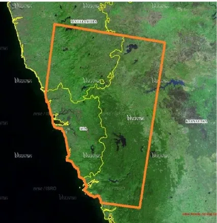
The study area chosen for this exercise is part of Western Ghats comprising the state of Goa, part of Karnataka and Maharashtra states of India. This area falls under UTM 43 zone in the northern hemisphere. The exact area of interest is shown as a
polygon in Figure 1. The total area is 17862 Sq. Km. and mostly covered by Western Ghats or Sahyadri mountain range. The average elevation of the area is around 1500 m with reference to MSL. This mountain range has a dense forest cover with many streams flowing through, which form the source for few major rivers of India like Godavari, Krishna and Kaveri. In this part of the country many reservoirs and dams were constructed in the last 3-4 decades over various streams.
Figure 1. Study area pertaining to part of Western Ghats, India (sourced from http://bhuvan.nrsc.gov.in)
The historical data set used for the study is Hexagon KH9 stereo pair from the mapping camera with a spatial resolution of 20 feet and acquired on 19 November 1973. The reference data includes CartoDEM with 10 m spacing (Muralikrishnan et al., 2013) for height control and Cartosat-1 orthoimages with a spatial resolution of 2.5 m for planimetric control in photogrammetric processing of Hexagon data. This reference data was generated from Cartosat-1 stereo pairs acquired in the month of December 2011.
4. PHOTOGRAMMETRIC PROCESSING Photogrammetric processing of Hexagon stereo data is not simple and straight forward due to non availability of interior orientation parameters of the mapping camera. Since the Hexagon and other photoreconnaissance missions were classified, the sensor details like principal point, fiducial marks, calibrated focal length were not known. Because of this interior orientation of these images for photogrammetric processing is considered to be difficult (Altmaier and Kany, 2002; Galiatsatos et al., 2008).
As per the hypothesis of Surazakov and Aizen (2010), the KH9 mapping camera of Hexagon was similar to Large Format Camera (LFC) flown onboard Space Shuttle mission STS 41-G (1984). This hypothesis was based on the fact that both the cameras were developed for space based topographic mapping by Itek Corporation. Based on this information a film based camera file is generated with a focal length of 304.8 mm and the format size of 230 mm X 460 mm. Each of the raw image for Hexagon was supplied in two pieces with a suffix a and b. These two parts of each frame was precisely registered one to one to make it a single frame image. On visual inspection of the ISPRS Annals of the Photogrammetry, Remote Sensing and Spatial Information Sciences, Volume II-8, 2014
stereo pair images it was inferred that the flying direction is along the longer dimension of the mapping camera. The principal point coordinates were assumed to be (0, 0). The four corners of the scanned images were taken as the fiducial marks for interior orientation and the fiducial coordinates were calculated based on the format size of the sensor. Thus the interior orientation of the raw images was carried out by measuring the four corners of the image that were treated as the fiducials for reference to recreate the internal sensor geometry.
Figure 2. KH9 Hexagon stereo pair with GCPs Exterior orientation tool of Inpho 5.7 photogrammetry software was used to estimate the initial values of the exterior orientation (EO) parameters for both the images. For this process, orthoimage and DEM generated using Cartosat-1 stereo data was used as the reference. These approximate EO parameters were imported into the project as GNSS and IMU values. The Hexagon KH9 images were initialized with these values. Automatic point matching tool of Inpho 5.7 was used to generate the tie points automatically. Prior to that few tie points were added manually to aid automatic point matching as there was a possibility of mismatches due to the presence of reseau grid marks on the images. Few sharp and common points were identified on both the Hexagon data and Cartosat-1 orthoimage to be used as the ground control. Triangulation of the stereo pair was carried out with 50 GCPs as shown in figure 2, which were extracted from the Cartosat-1 derived orthoimage and DEM. The stereo images were triangulated with a Root Mean Square Error (RMSE) of 2.5 m in X, 2.3 m in Y and 5.0 m in Z.
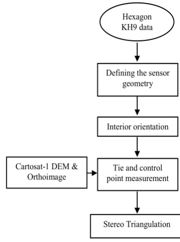
For Rational Function modelling, a grid of well distributed GCPs covering entire portion of the images are required to compute RPCs. For this the reseau grid marks available on Hexagon images were taken as the reference. First the Hexagon raw images were orthorectified with reference to Cartosat-1 orthoimage and DEM through projective transformation using the Autosync tool of Erdas Imagine 2014 software. The ground coordinates for each grid mark was extracted from the orthorectified Hexagon data. The ground coordinates for 98 grid points as shown in figure 3 and the corresponding image coordinates for each reseau grid mark were used to compute the RPCs. This computation was done using the program code written for the purpose in MATLAB 14a. These RPCs were used to orient the Hexagon stereo model in Imagine 2014 photogrammetry software. The accuracy of this stereo data was ascertained using independent, well distributed check points extracted from the reference data. The methodology adopted for orientation of Hexagon stereo data is depicted in the form of flowcharts through Figures 4 & 5. The model error values for the Hexagon stereo data by both rigorous sensor and RFM are given in Table1.
Figure 3. Grid of GCPs for RPC generation
Figure 4. Orientation of Hexagon data through RSM DEM was generated with a spacing of 50 m for the overlap area of the stereo pair through automatic point matching. Due to the presence of reseau grid marks and low contrast in few parts of the image data, the automatic point matching could not get the
Defining the sensor geometry
Interior orientation
Tie and control point measurement
Stereo Triangulation Hexagon KH9 data
Cartosat-1 DEM & Orthoimage
conjugate points at some places. Hence, DEM points were edited manually in 3D for further refinement. This refined DEM was used to generate orthoimage of the study area with a of 6 m.
Figure 5. Orientation of Hexagon data through RFM
Rigorous Sensor Model Rational Function Model Error X(m) Y(m) Z(m) X(m) Min 0.17 0.01 0.18 0.65 0.52 Max 5.37 7.07 12.02 6.58 5.07 RMS 2.51 2.28 5.04 2.32 3.75
Table 1. RMSE after adjustment through RSM and RFM 4.1 Change Detection
The orthoimage generated from KH9 Hexagon data was compared with the reference orthoimage from
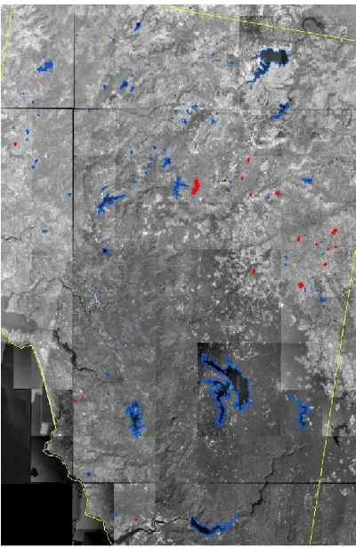
prominent changes in the study area. The main interest was to identify the water bodies, both minor and major that have been constructed on various streams during this temporal gap water bodies present in the study area were digitized on both the data sets using ARC GIS 10.2.1 software. The water digitized from Hexagon KH9 data acquired in 1973 are shown in red colour in Figures 6 and 7. The new water bodies after 1973 were digitized from Cartosat-1 data acquired in 2011 and they are depicted in blue colour in Figures
water bodies that were not present in Hexagon data were marked and segregated into a separate layer for further analysis The total number of new water bodies that have come up after 1973 was found to be 72 out of 89 in 2011. These new water bodies covered an area of about 2300 hectares
regarding the number of water bodies from both the data sets and the area covered by them are given in Table 2
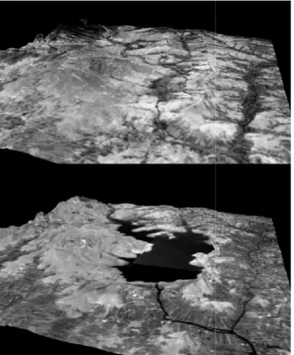
reservoirs in the study area i.e. Hidkal dam of Karnataka was not present in 1973 is shown in Figure 8
view on both Hexagon and Cartosat-1 data. RPC generation
Stereo Orientation Hexagon KH9 data
Georeferencing
Extraction of image & ground coordinates Cartosat-1 DEM
& Orthoimage
DEM points were This refined DEM rthoimage of the study area with a GSD
. Orientation of Hexagon data through RFM
Rational Function Model
Y(m) Z(m) 0.52 2.08 5.07 9.79 3.75 7.38 after adjustment through RSM and RFM
The orthoimage generated from KH9 Hexagon data was from Cartosat-1 for prominent changes in the study area. The main interest was to minor and major that have been temporal gap. The water bodies present in the study area were digitized on both the The water bodies from Hexagon KH9 data acquired in 1973 are shown water bodies built 1 data acquired in 2011 colour in Figures 6 and 7. All the re not present in Hexagon data were and segregated into a separate layer for further analysis. hat have come up after . These new water an area of about 2300 hectares. The details regarding the number of water bodies from both the data sets given in Table 2. One of the of Karnataka that as a perspective
Figure 6. Hexagon image with water bodies shown in red colour (digitized from Hexagon KH9 data of 1973) and blue polygons (new waterbodies digitized from
Cartosat-Figure 7. Cartosat-1 image with water bodies polygon were built between 1973 and 2011
Cartosat-1 data). RPC generation
Stereo Orientation Hexagon
data
Georeferencing
Extraction of image & ground coordinates
. Hexagon image with water bodies shown in red colour data of 1973) and blue polygons
-1 data of 2011).
ater bodies shown in blue built between 1973 and 2011 (digitized from ISPRS Annals of the Photogrammetry, Remote Sensing and Spatial Information Sciences, Volume II-8, 2014
Hexagon KH9
data (1973) Cartosat1 (2011 No. of water bodies 17
Area coverage (Ha) 1178.79
Table 2. Number of water bodies and the area covered in Hexagon and Cartosat-1 data
Figure 8. Perspective view of Hidkal dam area in 1973 (Hexagon-top) and 2011 (Cartosat-1-bottom
5. CONCLUSIONS
Historical data is a prime input for temporal studies using remote sensing technology. For most of the country, historic data in high resolution is not available for periods before Corona program after declassification make a great potential for change detection studies. This data provide us with invaluable historic record of spatial features and their environs which could be of special interest to various disciplines of science. But photogrammetric processing of these data sets is
non availability sensor interior geometry parameters. From the study it can be inferred that the hypothesis that mapping camera of Hexagon KH9 is similar in design with the Large Format Camera built by the same manufacturer holds good. Based on the information available and few assumptions
geometry could be successfully recreated. The presence of reseau grid marks on the hexagon data can create problems in automatic point matching. Care should be taken to identify and correct these mismatches in order to avoid the blunders. Inspite of these issues, an accuracy of better than one
achieved in adjustment of the Hexagon stereo data
RSM and RFM. The advantage of RSM is that it represents the true physical sensor geometry of a sensor. T
parameters in RSM have physical sense and
interpret. But the physical sensor geometry information is not always available. For historical data sets where sensor and platform related information is not available terrain depe RFM can be a good option. The main advantage of RFM is it is
Cartosat1 data (2011)
89 3479.19 Table 2. Number of water bodies and the area covered in
area in 1973 bottom)
input for temporal studies using remote sensing technology. For most of the country, historical data in high resolution is not available for periods before 80s. after declassification make a great potential for data provide us with invaluable historic record of spatial features and their environs which could be of special interest to various disciplines of science. But ing of these data sets is tedious due to availability sensor interior geometry parameters. From the study it can be inferred that the hypothesis that mapping camera is similar in design with the Large Format Camera built by the same manufacturer holds good. Based on n available and few assumptions, the internal The presence of grid marks on the hexagon data can create problems in automatic point matching. Care should be taken to identify and order to avoid the blunders. Inspite one pixel has been achieved in adjustment of the Hexagon stereo data using both The advantage of RSM is that it represents the . The geometry and are easy to interpret. But the physical sensor geometry information is not always available. For historical data sets where sensor and platform related information is not available terrain dependent The main advantage of RFM is it is
independent of sensor geometry and attitude
GCPs are available, RFM can provide accuracy similar to RSM. Comparison of Cartosat-1 data with KH9 Hexagon data provides an idea of the kind of changes that have taken place during the long period of time between 1973 and 2011 present study area a total of 72 water bodies have been built over various natural flowing streams covering an area of 2300 hectares after 1973. The implications of such changes need to be studied and understood in the
make better decisions for future growth.
6. ACKNOWLEDGEMENT The authors express their sincere gratitude to CSRE, IIT Bombay, for his critical evaluation
and valuable suggestions. Special thanks to Sri P. Srinivasulu, General Manager, AS&DMA, NRSC for his support during this study.
7. REFERENCES
Altmaier, A., Kany, C., 2002. Digital surface model generation from Corona satellite images. ISPRS Journal of Photogrammetry & Remote Sensing, 56 (2002)
Anderson, G, L., 2006. How to detect desert trees using Corona images: discovering historical ecological data.
Environments, 65(2006), pp. 491–511.
Campbell, J, B., Wyne, R, H., 2011. Introduction to Remote sensing. Guilford press, New York, pp. 159
Dashora, A., Lohani, B., Malik, J, N., 2007. A repository of earth resource information – Corona satellite program. CURRENT SCIENCE, 92(7), pp. 926-932.
Dashora, A., Sreenivas, B., Lohani, B., Malik, J
A., 2006. GCP collection for corona satellite photographs: Issues and methodology. Journal of the Indian society of remote sensing, 34(2), pp. 153-160.
Di, K., Ma, R. Li, X, R., 2003. Rational functions and potential for rigorous sensor model recovery, PE &RS, 6
Dowman, I., Dolloff, J, T., 2000. An evaluation of Rational functions for photogrammetric restitution.
Archives of Photogrammetry and Remo XXXIII, Part B3. Amsterdam.
Galiatsatos, N., Donoghue, D, N, M., Philip, G., 2008. High resolution elevation data derived from stereoscopic Corona imagery with minimal ground control: An approach using Ikonos and SRTM data. PE &RS, 74(9), pp. 1093
Grodecki, J., Dial, G., 2003. Block Adjustment of high resolution satellite images described by rational functions, PE &RS, 69(1), pp 59-69.
http://bhuvan.nrsc.gov.in/map/bhuvannew/bhuvan2d.php (Accessed on 03 June, 2014).
http://www.isro.org/satellites/earthobservationsatellites.aspx
(Accessed on 03 June, 2014).
independent of sensor geometry and attitude. If well distributed GCPs are available, RFM can provide accuracy similar to RSM. 1 data with KH9 Hexagon data an idea of the kind of changes that have taken place between 1973 and 2011. In the water bodies have been built covering an area of about er 1973. The implications of such changes the right spirit in order to
ACKNOWLEDGEMENT
The authors express their sincere gratitude to Prof. Y.S. Rao, , for his critical evaluation of the manuscript Special thanks to Sri P. Srinivasulu, General Manager, AS&DMA, NRSC for his support during this
REFERENCES
Altmaier, A., Kany, C., 2002. Digital surface model generation ISPRS Journal of 56 (2002), pp. 221 – 235. ., 2006. How to detect desert trees using Corona images: discovering historical ecological data. Journal of Arid
., 2011. Introduction to Remote sensing. Guilford press, New York, pp. 159-181.
., 2007. A repository of Corona satellite program.
932.
Dashora, A., Sreenivas, B., Lohani, B., Malik, J, N., Shah, A, GCP collection for corona satellite photographs: . Journal of the Indian society of remote
Rational functions and potential , PE &RS, 69(1), pp. 33-41. ., 2000. An evaluation of Rational functions for photogrammetric restitution. International Archives of Photogrammetry and Remote Sensing. Vol.
., Philip, G., 2008. High resolution elevation data derived from stereoscopic Corona imagery with minimal ground control: An approach using
pp. 1093–1106. Block Adjustment of high resolution satellite images described by rational functions, PE
an.nrsc.gov.in/map/bhuvannew/bhuvan2d.php
http://www.isro.org/satellites/earthobservationsatellites.aspx, ISPRS Annals of the Photogrammetry, Remote Sensing and Spatial Information Sciences, Volume II-8, 2014
Hu, Y., Croitoru. A., Tao, V., 2004. Understanding the rational function model: methods and applications. International Archives of Photogrammetry and Remote Sensing, 12-23 July, Istanbul, vol. XX, pp. 663-668.
Hussain, M., Chen, D., Cheng, A., Wei, H., Stanley, D., 2013. Change detection from remotely sensed images: From pixel-based to object-pixel-based approaches. ISPRS Journal of Photogrammetry and Remote Sensing, 80 (2013), pp. 91–106. Jianya, G., Haigang, S., Guorui, M., Qiming, Z., 2008. A review of multi-temporal remote sensing data change detection algorithms. The International Archives of the Photogrammetry, Remote Sensing and Spatial Information Sciences. Vol. XXXVII. Part B7. Beijing, pp. 757-762.
Kasturirangan, K., Aravamudan, R., Deekshatulu, B, L., Joseph, G., Chandrasekhar, M, G., 1996. Indian Remote Sensing satellite (IRS)-1C- the beginning of a new Era. Current science, 70(7), pp. 495-500.
Liu, S, J., Tong, X, H., 2008. Transformation between rational function model and rigorous sensor model for high resolution satellite imagery. The International Archives of the Photogrammetry, Remote Sensing and Spatial Information Sciences. Vol. XXXVII. Part B1. Beijing.
Ma, R., 2013. Rational Function Model in processing historical aerial photographs. PE &RS, 79(4), pp. 337-345.
Madani M, 1999. Real-Time Sensor-Independent Positioning by Rational Functions. Proceedings of ISPRS Workshop 'Direct versus indirect methods of sensor orientation', Barcelona, November 25-26, 1999. pp 64-75.
Muralikrishnan, S., Pillai, A., Narender, B., Reddy, S., Venkataraman, V, R., Dadhwal, V, K., 2013. Validation of Indian DEM from Cartosat-1 data. Journal of the Indian society of Remote sensing, 41(1), pp. 1-13.
Narama, C., Kaab, A., Duishonakunov, M., Abdrakhmatov, K., 2010. Spatial variability of recent glacier area changes in the Tien Shan Mountains, Central Asia, using Corona (~1970), Landsat (~2000), and ALOS (~2007) satellite data. Global and Planetary Change, 71 (2010), pp. 42–54.
Navalgund, R., Jayaraman, V., Roy, P, S., 2007. Remote sensing applications: an overview. Current science, 93(12), pp. 1747-1766.
NRO, 2011. Hexagon fact sheet. http://www.nro.gov/history/ csnr/gambhex/Docs/Hex_fact_sheet.pdf (Accessed on 31Oct, 2013).
Pieczonka, T., Bolch, T., Buchroithner, M., 2011. Generation and evaluation of multitemporal digital terrain models of the Mt. Everest area from different optical sensors. ISPRS Journal of Photogrammetry and Remote Sensing, 66 (2011), pp. 927– 940.
Pieczonka, T., Bolch, T., Junfeng, W., Shiyin, L., 2013. Heterogeneous mass loss of glaciers in the Aksu-Tarim Catchment (Central Tien Shan) revealed by 1976 KH-9 Hexagon and 2009 SPOT-5 stereo imagery. Remote Sensing of Environment, 130 (2013), pp. 233–244.
Shaoqing, Z., Lu, X., 2008. The comparative study of three methods of remote sensing image change detection. The International Archives of the Photogrammetry, Remote Sensing and Spatial Information Sciences. Vol. XXXVII. Part B7. Beijing, pp. 1595-1598.
Singh, S, K., Naidu, S, D., Srinivasan, T, P., Krishna, B, G., Srivastava, P, K., 2008. Rational Polynomial Modelling for Cartosat1 data, The International Archives of the Photogrammetry, Remote sensing and Spatial information sciences, Vol. XXXVII. Part B1. Beijing.
Surazakov, A., Aizen, v., 2010. Positional accuracy evaluation of declassified Hexagon KH9 mapping camera imagery. PE &RS, 76(5), pp. 603-608.
Tao, V., Hu, Y., 2001a. A Comprehensive study on the rational function model for photogrammetric processing, PE &RS, 67(12), pp. 1347-1357.
Wolf, P, R., Dewitt, B, A., 2004. Elements of Photogrammetry with applications in GIS. McGraw Hill, Boston, pp. 234-235. ISPRS Annals of the Photogrammetry, Remote Sensing and Spatial Information Sciences, Volume II-8, 2014