ANALYSIS
Environmental drag: evidence from Norway
Annegrete Bruvoll
a,*, Solveig Glomsrød
a, Haakon Vennemo
baStatistics Norway,P.O.Box8131Dep.,N-0033Oslo,Norway bECON,P.O.Box6823St.Ola6s Plass,N-0130Oslo,Norway
Received 22 January 1997; received in revised form 28 May 1998; accepted 19 October 1998
Abstract
Economic growth affects the environment negatively. A polluted environment and other environmental constraints reduce economic output and the well-being of consumers. The cost to society of environmental constraints may be called the environmental drag. The traditional economic analysis of growth neglects the environmental drag, while this paper attempts to measure it empirically. We employ a dynamic general equilibrium model of the Norwegian economy, extended to include some important environmental linkages, which feed back to the productivity of labor and capital from damages to health, materials and nature. The environment also directly affects the consumers’ well-being. Using this model, we are able to estimate the environmental drag, measured as reduced welfare from consumption and environmental services. We present macroeconomic effects in terms of reduced production and consumption, and calculate the overall welfare effects. We find that the environmental constraints incorporated in the model probably have a modest effect on production over the next century. The direct welfare loss from a degraded environmental quality, however, is significant. A lower rate of technological growth and a lower discount rate both increase the drag. © 1999 Elsevier Science B.V. All rights reserved.
Keywords:Environmental drag; Dynamic CGE model; Norway; Welfare effects JEL-classification: D58, O41, Q29, Q39
www.elsevier.com/locate/ecolecon
Nothing really matters much, it’s doom alone that counts.
Bob Dylan, ‘Shelter from the Storm’
1. Introduction
It is becoming increasingly appropriate to view the economic system as a growing subsystem within the ecological system, rather than an inde-pendent system with more or less infinite access to input and output. The need for a change of focus to a growing interdependence on the surrounding
* Corresponding author. Tel.: +47-2286-4948; fax: + 47-2286-4963.
E-mail address:[email protected] (A. Bruvoll)
nature was pointed out by Ayres and Kneese (1969), who argued that the production of residu-als (disposresidu-als from the consumption and produc-tion process) is an inherent and general part of the production and consumption process, and that partial equilibrium approaches may lead to serious errors.
The cost of environmental constraints on wel-fare is labeled theen6ironmental drag.1The overall
environmental drag can affect economic growth and total welfare in different proportions. It sur-faces as negative effects on health, vegetation, materials and consequently productivity, and im-plies a reduction in welfare from both the con-sumption of material goods and environmental services. The traditional economic analysis of growth neglects the environmental drag.
This paper addresses empirically the size of the drag on the Norwegian economy. The size of the environmental drag will be measured in terms of changes in welfare as well as effects on growth rates.
Earlier economic studies have provided valu-able theoretical contributions to the understand-ing of how the environment constrains economic development. For instance, Dasgupta and Heal (1974) show that when taking account of a drag from non-renewable resources, a steady state growth path only exists if the non-renewable re-sources are inessential in production. Tahvonen and Kuuluvainen (1993) show that a steady state path of an economy with pollution only is possi-ble in the case of a relatively low discount rate. For a more policy oriented discussion of the same issues, see Nordhaus (1992).
To estimate the environmental drag we employ a computable dynamic general equilibrium (CGE) model for Norway called DREAM (dynamic re-source/environment applied model). DREAM treats the economy and the environment as a simultaneous, extended dynamic general equi-librium system. There are linkages, in the form of environmental externalities, back and forth
be-tween the economy and the environment. The model integrates externalities associated with local air pollution and road traffic. Damages to health, materials, nature and congestion feed back to material welfare by reducing productivity of labor and capital. In addition, the environment matters directly to consumers as a good or service of its own, providing non-economic welfare to the soci-ety through opportunities for recreation, esthetic pleasure and personal well-being.
We compare two simulations. In the baseline scenario, we assume that there are no linkages between the environment and the economy. In the feedback scenario, based on the feedback model, we introduce the mutual dependence between the economy and the environment as an additional constraint on economic development. By compar-ing the difference in the outcome in the two scenarios, we are able to estimate the environmen-tal drag. Within our empirical feedback model framework, we also question the role of discount-ing, technical progress and energy prices in rela-tion to the environmental drag.
Stringent future regulation of environmental externalities can change the estimated environ-mental drag. At this stage we aim at estimating the worst case, given that no further political actions are taken. Thus our estimate of the drag is to be considered as a starting point with respect to further policy formation and decision making. As a disaggregated and general equilibrium model, DREAM reveals benefits and costs from reallocation of resources as a response to environ-mental damage or implementation of control measures. The dynamic feature further brings in the importance of consumers and producers look-ing forward, chooslook-ing between actions now or in the future.
To motivate our choice of model further we note that the relationship between the environ-ment and the economy is fundaenviron-mentally about interdependency and economywide linkages, i.e. it has a general equilibrium nature. Experiences with incorporating environmental costs in static CGE models suggest that the general equilibrium effects of environmental impacts can be significant compared with the estimated direct out-of-pocket expenditures (Alfsen, 1994). In some cases those general equilibrium effects are not as important,
but that is difficult to tell at the outset and in our case not necessary to accept by assumption. Dis-cussing this issue, Jorgenson and Wilcoxen (1993) recognize that the dynamic CGE model is a pow-erful tool for conducting medium to long-run applied economic analysis of energy and the envi-ronment. Predecessors in the related field of global models include the DICE model of Nord-haus (1993) and the model of Kverndokk (1993), both focusing the interdependence between eco-nomic activity and carbon dioxide emissions.
The paper proceeds as follows; Section 2 de-scribes our model, including the environmental linkages, and Section 3 presents the main set of results. Section 4 indicates effects of introducing some channels of interdependence of a more ex-ploratory nature, while Section 5 concludes and summarizes the analysis.
2. The model
DREAM is a computable dynamic general equilibrium model of Norway. (See Vennemo (1997) for a complete technical documentation). DREAM has earlier been used in cost-benefit analyses of emissions reductions (Olsen, 1995), tax reform implications (Vennemo, 1995) and to esti-mate the effects of green throughput taxation (Bruvoll and Ibenholt, 1998). The economic core model is a growth model of Cass – Koopmans type. The economy of Norway is reasonably close to a small, open economy, facing an exogenous interest rate and exogenous prices on competitive products. The model treats the economy and the ecology as a simultaneous system and thus opens for analysis of the environmental effects, in addi-tion to baseline economic effects. The model also computes the welfare effects of environmental quality and leisure time in addition to the welfare from baseline material consumption.
The annual trade balance reflects intertemporal optimization by consumers and producers. The trade balance changes temporarily with underly-ing economic conditions, but must comply with a financial restriction in the long term. This treat-ment is similar to current work in trade theory, see Obstfeld (1982) for an early contribution. All
agents have perfect foresight. We impose annual governmental budget balance, while a lump sum tax clears the budget. The transversality condition is a ‘non-Ponzi Game’, which implies that the stock of net foreign claim cannot grow at a rate higher than the interest rate as time goes to infinity, thereby limiting the consumers’ consump-tion possibilities.2
2.1. Production structure
The model includes six endogenous industries with competitive producers.3
The model also in-cludes two exogenous industries4 in addition to the public sector, all heavily regulated. Factors are mobile between sectors. Capital is internation-ally mobile, while labor is assumed immobile be-tween Norway and other countries.
The manufacturing industry produces trad-ables. Equality between price and unit cost in this industry determines the equilibrium wage rate in all sectors. This wage level in combination with the exogenous interest rate and self-fulfilling ex-pectations of the future prices of capital goods, determines the output prices of non-tradables.
Labor demand is determined such that the value of the marginal product of labor equals the price of effective labor input. An exogenous trend increases labor productivity, while production is adversely affected by the environmental impacts.
Output is produced in multi-level CES produc-tion funcproduc-tions. At the top level, material input and a capital-energy-labor composite combine into gross production. The elasticity of substitu-tion is zero; material input (including transport oils) is a fixed factor.5
2The model assumes that Ricardian equivalence holds, stat-ing that total savstat-ings will be unaffected by changes in govern-ment spending, since the houshold sector will change its savings correspondingly. In this case it is less interesting to focus on the state of public finances.
3Manufacturing goods, petroleum refining, construction, services, wholesale and retail trade, and housing.
4The production of crude oil and gas, and production of hydro-power.
Subsequent composites aggregate labor, capital and energy, while energy is a CES aggregate of fuel oil and electricity. The substitution elastic-ities, which differ among the ‘endogenous’ indus-tries of the model, are derived from Alfsen et al. (1996). Elasticities of substitution are generally below unity, indicating an inelastic production structure.
2.2. Consumption
The consumers are represented by an infinitely lived consumer who maximizes utility from full consumption (i.e. consumption of goods and leisure). Distributional issues are ignored. Prefer-ences are assumed to have a multi-level CES structure. Parameters are estimated on time series data for the Norwegian economy. The intertem-poral rate of substitution is 0.5, a value broadly consistent with econometric evidence in Norway (Biørn and Jansen 1982; Steffensen, 1989).
The consumers’ choice between labor and leisure is a function of the real wage. The income effect on labor supply is rather low, in accordance with empirical evidence for Norway (Dagsvik and Strøm, 1992). The uncompensated elasticity is 0.3 and the compensated 0.4.
A Cobb Douglas system spreads consumer ex-penditure on housing, tourism abroad and a man-ufacturing good, which includes gasoline and diesel associated with household transport, and captures the rest of commodities. With a given interest rate, consumption growth is determined.
2.3. En6ironmental feedbacks
The model tracks traffic volumes and emissions of seven pollutants to air. SO2 (sulfur dioxide) and NOx (nitrogen oxides) cause local pollution and contribute to the formation of acid rain, CO (carbon monoxide) and PM10 (particulate matter) cause local pollution problems, NMVOC (non-methane volatile organic compounds) generate ground level O3 (ozone), with local, regional and global environmental effects, while CO2 (carbon dioxide), N2O (nitrous oxide), NH3 (ammonia) and CH4 (methane) are important greenhouse gases. For each pollutant and industry, emissions
from mobile combustion, stationary combustion and industrial processes are assumed proportional to consumption of gasoline, fuel oil and material input respectively. Emissions from private con-sumption are proportional to households’ gaso-line and fuels consumption.
Three links from the environment to the econ-omy are identified. The first link concerns labor supply and labor productivity. Air pollution from SO2, NOx, CO and PM10and traffic noise damage health and leave people unable to work for a short or long spell, which together with a large number of traffic casualties, add up to a decrease in labor productivity in macro.
The second link concerns material damage; SO2 induces corrosion on capital equipment, and traffic wears down roads and increases road de-preciation and thus dede-preciation of public capital. This increased burden on public expenditures eventually crowds out private activity.
The third link concerns welfare. Consumers receive direct utility from environmental services, like recreational values. NOx and SO2 contribute to acidification of lakes and forests, exposure to NOx, SO2, CO and PM10 results in health-related suffering, and traffic involves annoyance from congestion, noise and traffic accidents. The con-sumers treat this utility component as a datum (external effect).
Marginal damage estimates refer to the base year. In the model, feedbacks from the environ-ment to the productive sphere are characterized by decreasing marginal damage, while the mar-ginal welfare effect to consumers is assumed to be constant. Pollution and traffic loads rise above the base year level in all growth scenarios. This might lead us to underestimate the drag associated with economic growth. On the other hand, constant marginal welfare effects might overstate the benefit of reaching zero pollution.
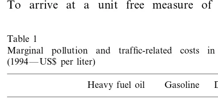
road traffic costs added up to around US$ 1.2 per liter of gasoline and 1.5 per liter of diesel. See Table 1 and Brendemoen et al. (1992) for further details.
Since the effect of Norwegian economic activity on global environmental changes are rather negli-gible, the model does not include feedback from the global environment. Also, it is assumed that economic actions in Norway do not influence trans-national pollution. Trans-national pollution is implemented as a constant in the utility function.
In Appendix A we outline the detailed incorpo-ration of the various environmental links in the core model and the underlying sources.
2.4. Welfare indicators
The welfare function is additive in welfare from full consumption (goods and leisure) and welfare from environmental services. Due to this specifi-cation, consumers’ trade-offs between leisure and work, and consumption versus saving, are not directly affected by environmental feedbacks. However, the feedbacks affect the prices facing consumers. The consumers respond by adjusting demand for consumption, leisure and savings.
Changes in welfare are measured by equivalent changes in (human plus financial- and real-capi-tal) wealth, i.e. the welfare change of a price increase is measured by the equivalent change in wealth at the original set of prices. This is the equivalent variation method in a dynamic context. To arrive at a unit free measure of welfare
change, we divide equivalent variation by the baseline scenario wealth.
2.5. Baseline input
The baseline input is used by the Ministry of Finance for the most recent long-term projection of the Norwegian economy (Ministry of Finance, 1993). From 2030 on, the exogenous values are assumed to be consistent with a steady state. See Olsen and Vennemo (1994) for more details on the baseline input.
The simulations are run for 101 years from 1989 to 2090. By 2090 the economy is approxi-mated by a steady state path that continues into infinity. We mainly discuss the period from base year 1989 until 2030, but we will also comment on some interesting steady state results. The reason for focusing on 2030 is that this period corre-sponds to the time horizon frequently used in medium- and long-term analyses of the Norwe-gian economy. In steady state, long-run growth converges to 2% annually, which is the rate of exogenous labor saving technical change. It takes the economy of the baseline model around 35 years to reach an approximate steady state, while it takes longer time in the feedback model.
3. Comparing the models: main results
We now compare the outcome of the feedback model with the baseline model. Total welfare, including welfare from the environment, is re-duced by 9.95%, mainly due to less welfare from the environment. The overall en6ironmental drag,
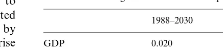
defined as the annual reduction in welfare growth, is estimated to 0.23%. Due to environmental feed-backs, annual production growth in the period 1988 – 2030 is reduced by 0.02 percentage points and consumption growth by 0.03 percentage points. The rest of the reduction in welfare growth is due to welfare from environmental services.
We now turn to a more detailed description of the main results, before we turn to the underlying effects explaining the difference between the feed-back model and the baseline model.
Table 1
Marginal pollution and traffic-related costs in Norway (1994 — US$ per liter)
Diesel Gasoline Heavy fuel oil
0.06 0.33
Health 0.57
0.24 Traffic accidents 0.00 0.21
0.09
Traffic noise 0.00 0.10
0.24 0.23
0.00 Congestion
0.00
Road damage 0.29 0.32
0.01 0.00
Corrosion 0.00
1.47 1.15
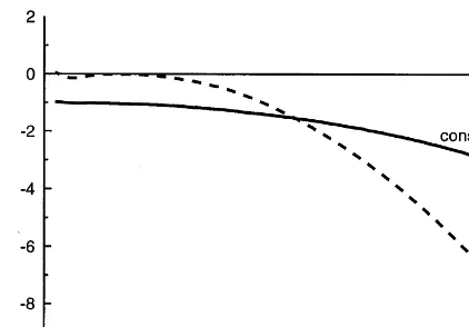
Fig. 1. Time paths for GDP and consumption. Percentage difference between baseline model and feedback model.
9.19% of total intertemporal wealth. That means that to have zero pollution, noise etc. would be equivalent for the consumers to a 9.19% increase in wealth, which could finance a 9.19% annual increase in the level of full consumption. Trans-formed into annual growth reductions required to reach 9.19% by 2030, the drag from environmen-tal services is 0.22%.
Table 2 provides a break-down of welfare loss from environmental services due to health dam-ages, congestion, traffic accidents and noise.
The health damages increase by 28% from 1989 up to 2030, while the other damage factors, con-gestion, traffic accidents and noise, increase by 92%. Health damages from emissions are the most important damage factor, and contribute to 39% of the total disutility from environmental services in 2030. The other main cost components are congestion and traffic accidents. Traffic related costs contribute to about one-half of the total estimate. By contrast, domestic contributions to acidification of lakes and forests are insignificant in the total estimate.
The intertemporal full welfare difference (dis-counted over the infinite time horizon) between the baseline and feedback worlds is 9.95% of welfare, or 110 billion US$. The annual growth rate of wealth required to reach 9.95% by 2030 is 0.23%, indicating the overall en6ironmental drag.
Our welfare indicator does not of course in-clude every subject that contributes to a society’s welfare. Of the seven emission components pro-jected by the model, CO2, CH4 and NMVOC do not have any formal welfare impact in the model. One might nevertheless find that the 80% increase in CO2 emissions until 2030 adds to the environ-mental drag. Emissions of CH4, another green-3.1. Welfare
Recall that the arguments of our money metric welfare function are a linear combination of full consumption (consumption of baseline goods and services and leisure) and environmental services. Welfare is intertemporal, i.e. it is a statistic of consumption of goods/services, leisure and envi-ronmental services over the entire infinite time-span.
If consumption of goods and services was the only argument of the welfare function, we would expect a welfare loss from environmental feed-backs in the range of 2-3%, which is the average consumption decrease (Fig. 1). But part of the reason why consumption and production are re-duced in the feedback scenario is that labor sup-ply decreases. That is to say that people purchase more leisure time in the feedback world, of which the partial effect is higher welfare. The total effect on full consumption (goods/services and leisure taken together) is a welfare loss, which is to be expected. The net effect of accounting for the environment in the production process is after all to impose additional costs on the economy. The intertemporal net welfare loss from full consump-tion, due to the effect of the environmental feed-backs into production, is 0.76%.
To get the full picture, we must however add the welfare loss from lower environmental ser-vices, which is far more important than welfare loss from full consumption, and amounts to
Table 2
Percentage distribution of disutility from lower environmental services in 2030
%
Health damages 39
31 Costs of congestion
house gas, also increase. Premature deaths in traffic accidents is another variable relevant to welfare. According to the model, accumulated traffic deaths reduce the population of 2030 by 7700, while the number of person injuries rise from 33 000 in 1989 to 67 000 in 2030. These numbers hide suffering and grief of great welfare importance. Our model by contrast treats non-fa-tal accidents and injuries as an issue of resource costs only, while a fatal injury to one of n mem-bers of the population is represented in the model as the removal of 1/n of total utility.
3.2. GDP and consumption
The fall in labor supply and capital contributes to a lower GDP level in the feedback scenario. In 2030 GDP is 0.82% lower than in the baseline scenario. The GDP gap grows over time because productivity gradually declines compared with the baseline scenario. The difference reaches 8.8% by 2090 (Fig. 1).
The lower GDP level of the feed-back scenario lowers income and consumption possibilities. In 2030, the value of private consumption in the feedback scenario is 1.4% lower than in the base-line scenario. This is larger than the correspond-ing loss in GDP because the consumers spread the income fall over the entire period. The timing of the production drag is not important because of perfect foresight and arguments equivalent to Richardian Equivalence. The immediate (base year+1) fall in consumption is 1.0%, while the long-run fall towards the end of the next century is 3.5%.
The GDP and consumption reductions also re-duce fossil fuels consumption, which again lowers emissions. This induces positive second order en-vironmental effects, which reduce the environ-mental costs. Table 3 verifies that environenviron-mental feedbacks reduce annual growth in GDP by 0.02 percentage points in 2030. Since the growth of the GDP gap increases, the growth rate reduction is larger in the long run.
The consumption growth rate is reduced by 0.03 percentage points in 2030. This reduction is not, however, significantly more pronounced in the long run. It is clear from looking at Fig. 1 that
Table 3
Environmental drag on GDP and consumptiona
1988–2030 1988–2090
GDP 0.020 0.092
0.033 0.036
Consumption
aDifference in annual growth between baseline scenario and feedback scenario. Percentage points.
the measured drag on consumption would have been larger if we examined a shorter period (i.e. 1988 until 2000), since there would have been fewer years by which to spread the reduced consumption.
3.3. Trade balance
The trade balance changes as a consequence of the adjustments to environmental feedbacks. In the first years, when consumption is decreased relative to production, the economy runs a trade balance surplus compared with the solution of the baseline scenario. Over time this trade balance surplus increases interest income from abroad, which opens the way for a long-term trade bal-ance deficit. Thus it is possible for consumers to maintain a relatively higher consumption level in the long run, ‘paid for’ in earlier years.
3.4. Emissions and fuel consumption
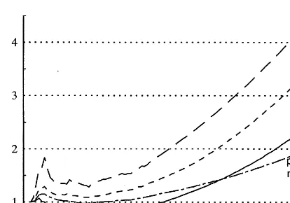
Fig. 2 shows a 101-year time path for the pollutants that cause welfare loss and feedbacks in the model: SO2, NOx, CO and PM10. An increased activity level over time doubles gasoline and diesel consumption from 1989 to 2030, as transportation demand increases with income. The growth in transportation helps to explain the welfare loss from environmental services. Consumption of heating fuel oil also doubles in this period.
Fig. 2. Time path of SO2, NOx, CO and particulate matter, 1989=100.
compared with the baseline scenario) by 0.15% in 2030. Depreciation of public capital (roads) has increased 56% by then, from a low base-value of about 0.75% annually. The increase in the depre-ciation of private capital, i.e. buildings and struc-tures, influences wages through the requirement that price equals cost. Depreciation of public cap-ital increases public consumption, which crowds out private consumption.
The increase in the user cost of capital in the competitive industry is 0.02% by 2030. The change in user cost is smaller than the change in depreciation of buildings and structures since de-preciation is only one aspect of the user cost of capital. The increased capital cost depresses the price of effective labor by 0.01% in order to keep overall costs constant in the competitive sector. This is less than capital costs increase, since the cost share of labor is larger than the cost share of capital. Intuitively, the fall in the wage can be spread thinner than the corresponding increase in the user cost of capital.
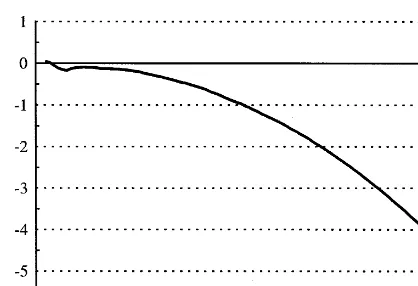
Fig. 3 shows the time path of the difference in labor productivity between scenarios over 101 years. In 2030, the difference is 0.8%, and growing exponentially to 5.2% by 2090. The reason for the exponential growth is that emissions, consump-tion of gasoline and diesel and road traffic all grow exponentially in steady state. Over the rele-vant range, there is an almost linear relation between productivity and its environmental deter-minants over the next century.
some specific sources diminishes over time. Abate-ment in transportation lowers the NOx and CO emissions growth. Abatement in industries to-gether with the introduction of cleaner, less sul-fur-intensive fuel-oils contribute to a lower SO2 emission growth. A large share of PM10 and CO emissions is tied to exogenous and constant use of fire-wood.
The reason for the long-run exponential path is that in the steady state all emission carriers ap-proach a growth rate equal to the 2% rate of labor saving technical progress. Emissions also grow by this rate, as there is no increase in abatement beyond current plans. In other words, we do not impose the inverted U-shape between emissions and growth that has been detected in historical data in some recent studies, e.g. Gross-man and Krueger (1995). The increase in emis-sions explains part of the welfare loss of environmental services. It also explains the in-crease in depreciation and fall in labor productiv-ity.
3.5. Depreciation,producti6ity and wages
Table 4 shows the difference in depreciation, user cost of capital, price of effective labor, pro-ductivity and wages in the feedback scenario com-pared with the baseline scenario for the years 2030 and 2090.
Corrosion is estimated to increase the deprecia-tion rate of buildings (in the feedback scenario
Table 4
Percentage difference between the feedback scenario and the baseline scenario, 2030 and 2090
2030 2090
Depreciation rate, buildings in trad- 0.15 1.54 ables industry
55.80
Depreciation rate, roads 58.04 0.02 0.21 User cost of capital in tradables
industry
Price of effective labor −0.01 −0.13 −0.76
Productivity −5.20
−0.77
Fig. 3. Percentage difference in productivity between baseline model and feedback model, 1989 – 2090.
Gross investments are affected in two ways as well: first by the corrosion-induced need to re-place, maintain and repair a greater share of capital as corrosion sets in, and second by the economy’s response to environmental feedbacks in the form of lower demand for capital. In most of the period before 2030, gross investment in-creases as the replacement effect is the most im-portant. Later on, gross investment decreases markedly because of the general equilibrium response.
By describing the effect on factor supplies, we have come full circle, as we started this story by explaining how lower factor supplies lowered con-sumption and GDP.
4. Sensitivity analysis
This section investigates some sources of envi-ronmental drag which are especially relevant from an environmental point of view. Crucial questions in the environmental debate are: Whether conven-tional economic analysis uses a too high discount rate, whether the assumed rate of technical pro-gress is too high, and whether energy prices will increase more than projected at the moment. Table 6 summarizes the results of the sensitivity analysis.
4.1. A lower discount rate?
Environmentalists sometimes claim that a high social discount rate is unfavorable to environmen-tal concerns by ignoring the future damage to the ecosystem associated with investment projects. However, the role of the discount rate in addressing the environmental costs is ambiguous when the effect of discounting on capital accumulation is taken into account. As pointed out by Krautkrae-mer (1988), a low discount rate encourages conser-vation of nature, but at the same time stimulates accumulation of production capital, which indi-rectly demands increasing amounts of natural re-sources. The trade off between welfare from these two types of wealth (capital and nature) must be assessed empirically. We take up this issue in two ways.
3.6. Labor and capital
Table 5 indicates the impact on labor and capital input. In 2030, labor supply is 0.3% lower in the feedback scenario, while it is 3.1% lower by 2090. The world with environmental drag is one where we work less than we would have done otherwise, since we receive a lower wage per hour. When measured in effective units, which is what matters for produc-tion, labor input is 1.2% lower in year 2030.
Capital input is lowered by 1.3% in 2030, due to a combination of two effects: One is a substitution effect from more expensive capital into cheaper labor: the fact that capital becomes more expensive relatively to labor encourages firms to hire more labor and reduce their demand for capital. The substitution effect occurs per unit of output. The other, and quantitatively more important effect, is that the scale of production goes down, which decreases the demand for real capital at given prices.
Table 5
Environmental drag on labor and capital inputa
1989–2030 1989–2090
Labor supply −0.3 −3.1
−1.2 −9.2
Effective labor input
−1.3
Capital input −8.0
−0.2 −12.0 Investment
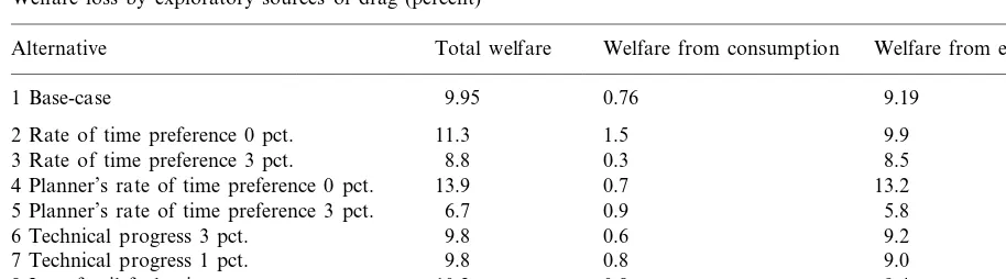
Table 6
Welfare loss by exploratory sources of drag (percent)
Welfare from consumption Welfare from environment
Alternative Total welfare
9.19
1 Base-case 9.95 0.76
9.9 2 Rate of time preference 0 pct. 11.3 1.5
3 Rate of time preference 3 pct. 8.8 0.3 8.5
13.2 4 Planner’s rate of time preference 0 pct. 13.9 0.7
5.8 5 Planner’s rate of time preference 3 pct. 6.7 0.9
6 Technical progress 3 pct. 9.8 0.6 9.2
9.0 7 Technical progress 1 pct. 9.8 0.8
8 Low fossil fuel price 10.2 0.8 9.4
9 High fossil fuel price 9.5 0.7 8.8
In alternatives 2 and 3, we investigate the con-sequence of changing the subjective rate of time preference in the model to 0 and 3%, which changes the world discount rate. The discount rate is of course higher than the rate of time preference, since consumption increases over time. The base-case subjective rate of time preference is 1%.
In our case the environmental drag increases with a low discount rate. This is not a simple story of valuing more highly a given amount of future environmental damage. Future environ-mental damage is not given, it is lower when the discount rate is lower. In fact, as Table 6 shows, welfare loss from the environment is not signifi-cantly different from the base-case, and the differ-ence that is observed may be related to the welfare loss to consumption, which we now proceed to explain: The main impact of a lower discount rate is to change the consumers’ trade-off between consumption now and in the future. That is the case for both scenarios, but the impact is greater in the feedback scenario: recall that the consumer of the feedback scenario hedged against the future impact of production drag by saving some of the early income. The reward to this action is reduced by a lower discount rate, thus the consumers must save more early on in order to enjoy the same steady state consumption level later. Thus to mo-bilize savings in order to meet the drag is more costly under a lower discount rate, increasing the welfare loss from consumption.
Consumers partly respond to the strain on the current account by working more, which increases
production and modifies the fall in intertemporal consumption. This increase in production, how-ever, harms the environment, increasing the envi-ronmental drag and the welfare loss from environment. On the other hand, a lower interest rate reduces the user cost of capital, and leads to more capital intensive and less energy intensive production, which modifies the scale effect on the environment. Hence, in our case, the more costly saving together with the production scale effects dominate the drag modification obtained through less energy and emission intensive production.
The next argument regarding the discount rate that we take up is the following: When society evaluates the result of an economic process, it may be desirable or reasonable to employ a lower discount rate than the members of society do as single economic agents. One reason that has been advanced is that individual agents do not care enough for their descendants, while another point of view is that society should employ a lower interest rate in the lack of first best instrument to combat environmental problems. The idea that utility should not be discounted in welfare evalua-tions goes back a long way (see e.g. Ramsey (1928)).
Alternatives 4 and 5 concern the impact of evaluating the economic outcome from a plan-ner’s point of view by 0 or 3% rate of time preference.6 This is a simple story of valuing the future more highly. The impact on welfare from
full consumption is small because of consump-tion smoothing which implies that the largest losses in full consumption do not necessarily come last. The largest impact is on welfare from the environment. A low planner’s rate of time preference puts more emphasis on the long-run damages than the consumers do themselves. Disutility from lower environmental quality in-creases 45% (4 percentage points) according to the preferences of the planner. In the same way, a high planner’s rate of time preference dis-counts high future damages more, reducing the impact on intertemporal utility.
4.2. Lower technological progress?
Environmentalists sometimes accuse the stan-dard economic analysis of assuming too high future technological progress and consequently an easy way out of many environmental prob-lems. Alternatives 6 and 7 evaluate how techno-logical progress affects welfare losses. Reducing the rate of technical progress will reduce the steady state interest rate, since the interest rate is linked to steady state consumption growth from the Euler – equation. This contributes to an increased welfare loss from consumption, similar to the higher loss of a low rate of time prefer-ence.
A low rate of technical progress over time also implies a smaller production scale, which in turn implies lower energy consumption and lower pollution, which in turn contributes to a lower loss in welfare from consumption in the feedback scenario. Thus reducing the rate of technical progress has two opposing effects on welfare from consumption: the interest rate ef-fect increases, while the scale efef-fect decreases the loss. The strengths of these effects are non-sym-metric around the base-case.
In terms of welfare from the environment, reduced technical progress implies lower emission growth and lower disutility from re-duced environmental services. The effect on emissions is modified by the increased work ef-fort that is part of the answer to lower interest rates.
4.3. Increasing energy prices?
Environmentalists are concerned that energy prices in the long run will increase more than assumed by the standard analysis. The baseline input assumes a 14% growth in real fossil fuel prices by 2030. What is the impact on the envi-ronmental drag of assuming higher (and lower, for comparison) fossil fuel prices? That is the topic of alternatives 8 and 9. By ‘higher’ we mean 2.5% annual growth. ‘Lower’ means zero growth.
Higher prices of fossil fuels imply that pro-ducers move into a more energy efficient mode of production. Emissions per unit of output fall. In addition the level of output falls because lower wages (remember they adjust to keep overall costs down) and labor supply means a contraction of the economy. All in all, emissions fall, which reduces the disutility from pollution.
A conclusion to the sensitivity analyses is the following: The results are robust with respect to a lower market rate of time preference. The ef-fect of a lower planner’s rate of time preference is significant, but not dramatic. The results are robust to energy prices and technical progress. Some of the effects that we do detect run against popular wisdom. For instance, endowing agents with a lower rate of time preference in-creases the environmental drag through its effect on labor supply.
4.4. Robustness
5. Conclusions
This analysis shows that environmental con-straints so far incorporated into production prob-ably have a modest effect over most of the next century. This conclusion is robust to a number of alternative specifications of parameters and exoge-nous variables. In fact, the welfare cost of full consumption (consumption of goods and leisure) shows a rather remarkable stability across differ-ent assumptions. However, the direct loss of wel-fare from the environment is significant. This conclusion is also robust to a number of alterna-tive specifications of parameters, with the excep-tion of the parameters that attribute welfare to environmental services.
The study indicates that the environmental drag on production reduces annual economic growth rates by about 0.1 percentage point. Annual growth in wealth, including environmental wealth, is reduced by 0.23 percentage points until 2030.
Our results can be compared to those of Nord-haus (1992). NordNord-haus estimates the drag from non-availability of cheap resources and from local pollutants. Our estimate for Norway only covers a limited number of acknowledged feedbacks from local pollution, but still comes out with twice the Nordhaus drag on economic growth. Costs re-lated to road traffic volume that are included in our study, but not among local pollutants consid-ered by Nordhaus, can partly explain the difference.
Our results can be used to indicate the benefits of abatement and related activities. If all the specified sources of environmental problems were eliminated by year 2030, GDP in that year would be 1.7 billion US$ higher (ignoring intertemporal reallocations). If all environmental problems were eliminated today, the total intertemporal welfare gain would amount to 110 billion US$. As we have seen, these are small sums in percentage terms, but they are pretty large sums in the con-text of abatement. Full abatement or elimination of all environmental problems will obviously not be cost effective, but a large number of abatement measures would probably pass the cost-benefit test. In a study of the US, Jorgenson and Wilcoxen (1990) find that environmental
regula-tion reduced the annual economic growth by 0.2 percentage points over the period 1974 – 1985, and the long-run reduction in growth significantly lower. Assuming a rational political process, one can interpret this as an estimate of the willingness to pay for avoiding environmental drag. Willing-ness to pay (for environmental improvements) of this magnitude would roughly match the level of environmental costs estimated in this paper so far in Norway.
The results of this paper are subject to a num-ber of qualifications. The global environmental linkages might be more important than the local linkages. Global environmental problems like the greenhouse effect are external to the Norwegian economy, and thus these are absent from the study, since they would affect both the baseline and feedback scenarios equally. Regarding the effects we find on production growth, there may be crucial interactions between the environment and the economy that we have not accounted for. Health impacts of current chemical flows are not yet fully understood or recognized. Relevant sub-jects of serious concern are carcinogens, hormone-mimicking compounds and anti-bacterial agents. Also, long term effects on productivity of land and marine environment are potential sources of drag that are not accounted for in our analysis.
We have assumed that the unit value of envi-ronmental damage is constant. This is doubtful, as the value may change with the level of damage as well as with income or just with time, and the estimation of non-market environmental goods is also riddled by a range of theoretical and practical problems. In addition we assume no technical improvement in abatement technology, which might contribute to overstating the environmental drag.
Overall, our estimate of the environmental drag is uncertain and based on a number of underlying assumptions that some readers may find uncon-vincing. These assumptions notwithstanding we think our numerical results are indicative of the size of the drag, and that the mechanisms we have described are important determinants of the envi-ronmental drag.
finance to generate efficient environmental and economic policy options. To bridge a gap between environmental and financial policy spheres, an integrated assessment of the environmental drag is clearly useful.
Acknowledgements
We are grateful to K.H. Alfsen, K.A. Brekke, E. Holmøy and two anonymous referees for use-ful comments.
Appendix A. Environmental feedbacks
We summarize the main principles and sources behind the incorporation of the environmental links into the core model. The parameters describ-ing the interaction between the economy and the environment are difficult to pin down, for obvious reasons. Our parameter values serve as illustra-tions rather than precise estimates. Further details and actual equations are documented in Vennemo (1997).
A.1. Emissions and traffic
The emission coefficients are calibrated to base-year data on emissions by source and industry relative to the relevant emission carrier. Exoge-nous abatement reduces the emission coefficients over time. The reduction in emission coefficients due to exogenous abatement is projected accord-ing to estimates from the Norwegian Pollution Control Agency. We use gasoline and auto-diesel consumption to proxy traffic volume. The argu-ment is that efficiency, demographic variables and security measures being constant, the change in gasoline and auto-diesel consumption captures the change in traffic-related externalities reasonably well. Traffic costs include accidents, congestion and noise and rise proportionally to traffic vol-ume. About half of external cost associated with gasoline and diesel consumption originate from traffic, not pollution per se.
The level of environmental and traffic-related costs included in this study can be illustrated as
marginal costs of using various fuels. The exter-nalities per liter of diesel and gasoline amount for about US$ 1.5 and US$ 1, respectively. Light and heavy fuel oil incur external costs of about US$ 0.02 and US$ 0.8 per liter, respectively (see Bren-demoen et al. (1992)).
A brief presentation of an updated version is provided by Alfsen and Rosendahl (1996), while a comprehensive documentation can be found in Rosendahl (1998).
A.2. Depreciation and producti6ity
Brendemoen et al. (1992) provide data on the relation between SO2 and corrosion costs associ-ated with buildings and similar capital assets. Cost estimates are based on dose-response func-tions and material inventories as documented in Glomsrød (1990). Pollution included corrosion also harms buildings and monuments of cultural value. This effect, while probably important, is not included in the model for data reasons. We assume that the amount of traffic is a reasonable proxy for the determinants of road depreciation.
Brendemoen et al. (1992) provide data on the environmental effects on labor productivity. The bottom line is an expert panel appointed by the Norwegian Pollution Control Agency that esti-mated the productivity cost of one person being above the WHO threshold level of pollution from SO2, NOx, CO and PM10, respectively. Dispersion models for emissions to air have been used to identify the number of people exposed to higher than threshold levels of pollution as emissions increase above the base year level. Only urban emissions are assumed to do harm.
average remaining working life for the perma-nently injured or dead would have been 37 years.
In a long-run model, we face the question of what happens if emissions affecting the supply of labor and capital grow without bounds. The model imposes upper bounds on the emissions’ impacts, which for capital depreciation is as-sumed to be 7.5%, three times the actual base-year rate of depreciation (of buildings and roads). For labor productivity loss, the maxi-mum is assumed to be 3% for NOx and PM10, and 1.5% for SO2 and CO, while the upper boundary for productivity loss from traffic noise is set to 1%. None of the maxims are binding within the first 101 years of the feedback sce-nario.
A.3. Welfare from en6ironmental ser6ices
The monetary cost estimates from Brende-moen et al. (1992) can be directly compared with monetary gains in consumption or wealth. We assume constant marginal costs of degrada-tion as a first approximadegrada-tion, as the data quality at the moment precludes any sophisticated mod-eling. Our cost estimates are uncertain even as marginal cost approximations, but they do indi-cate a likely magnitude. Somewhat arbitrarily we claim the welfare cost of air pollution to be one-half the productivity cost, which may well be an underestimate.
Estimates of external costs of road traffic (road damage, noise and congestion) are based on studies by the Norwegian Pollution Control Agency and concern the capital, Oslo. The geo-graphical allocation of a given increase in traffic volume is important when calculating external costs from traffic. We assume that 30% of traffic causes congestion costs, corresponding to the ten largest Norwegian cities’ share of total diesel and gasoline consumption in the model base year. Traffic accidents are more reasonably related to all traffic. The welfare cost of traffic accidents is quite prosaic as measured by the model: It consists of estimated medical penses, material expenses and administrative ex-penses.
References
Alfsen, K.H., 1994. Natural resource accounting and the analysis in Norway, Documents 94/2, Statistics Norway. Alfsen, K.H., Bye, T., Holmøy, E. (Eds.), 1996. MSG-EE:
An applied general equilibrium model for energy and environmental analysis, Chapter 3, Social and economic studies no. 97, Statistics Norway.
Alfsen, K.H., Rosendahl, K.E., 1996. Economic damage of air pollution, Documents 96/17, Statistics Norway. Ayres, R.U., Kneese, A.V., 1969. Production, consumption,
and externalities. American Economic Review LIX, 282 – 297.
Biørn, E., Jansen, E., 1982. Econometrics of incomplete cross-section/timeseries data: Consumer demand in Nor-wegian households 1975 – 1977, Samfunnsøkonomiske Studier 52, Statistics Norway.
Brendemoen, A., Glomsrød, S., Aaserud, M., 1992. Miljøkostnader i makroperspektiv (Environmental costs in a macro-perspective), Rapporter 92/17, Statistics Nor-way.
Bruvoll, A., Glomsrød, S., Vennemo, H., 1995: The Envi-ronmental Drag on Long-term Economic Performance: Evidence from Norway, Discussion Papers 143, Statistics Norway.
Bruvoll, A., Ibenholt, K., 1998: Green throughput taxation. Environmental and economic consequences. Environ. Re-sour. Econ. 12(4), 387 – 401.
Dagsvik, J.K., Strøm, S., 1992. Labour supply with non-convex budget steps, hours restrictions and non-pecu-niary job-attributes, Discussion Papers 76, Statistics Norway.
Dasgupta, P., Heal, G., 1974. The optimal depletion of ex-haustible resources. Rev. Econ. Stud. (Symposium), 3 – 28.
Glomsrød, S. 1990. Some macroeconomic consequences of emissions to air. In: Fenhann, J. et al. (Eds): Environ-mental Models: Emissions and Consequences. Proceed-ings from Risø International Conference 1989. Elsevier, Netherlands.
Glomsrød, S., Nesbakken, R., Aaserud, M., 1998. Modelling impacts of traffic injuries on labour supply and public health expenditures in a CGE framework. In: K.E. Rosendahl (Ed.), Social Cost of Air Pollution and Fossil Fuel Use — A Macroeconomic Approach, Social and Economic Studies 99, Statistics Norway.
Grossman, G.M., Krueger, A.B., 1995. Economic growth and the environment. Q. J. Econ. 110(2), 353 – 379. Jorgenson, D.W.I., Wilcoxen, P., 1990. Intertemporal general
equilibrium modelling of US environmental regulation. J. Policy Modelling 12 (4), 715 – 744.
Jorgenson, D.W., Wilcoxen, P., 1993. Energy, the environ-ment and economic growth. In: Kneese, A.V., Sweeney, J.L. (Eds.), Handbook of Natural Resources and Energy Economics III, pp. 1267 – 1390.
Kverndokk, S., 1993. Global CO2agreements: a cost-effective approach. Energy J. 14 (2), 91 – 111.
Ministry of Finance, 1993. Langtidsprogrammet 1994 – 1997, St.meld. nr. 4 (1992 – 93) (Report no. 4 to the Storting (1992 – 1993): Long-term program 1994 – 1997). (Parts of the report are available in English)
Nordhaus, W., 1992. Lethal model 2: the limits to growth revisited. Brookings Papers Econ. Activity 2, 1 – 59. Nordhaus, W., 1993. Rolling the ‘DICE’: an optimal transition
path for controlling greenhouse gases. Resour. Energy Econ. 15, 27 – 50.
Obstfeld, M., 1982. Aggregate spending and the terms of trade: is there a Laursen – Metzler effect. Q. J. Econ. 97, 251 – 270.
Olsen, K., 1995. Nytte- og kostnadsvirkninger av en norsk oppfyllelse av nasjonale utslippsma˚lsettinger (Cost- and benefit implications of a Norwegian fulfilment of national emission targets), Notater 95/7, Statistics Norway. Olsen, K., Vennemo, H., 1994. Formue, sparing og vekst:
en analyse av langtidsprogrammets perspektiver (Wealth, savings and growth: an analysis of the perspectives of the Long-term programme). Sosialøkonomen 9, 32 – 38.
Ramsey, F.P., 1928. A mathematical theory of saving. Econ. J. 38, 543 – 559.
Rosendahl, K.E., 1998 (Ed.). Social Cost of Air Pollution and Fossil Fuel Use — A Macroeconomic Approach, Social and Economic Studies 99, Statistics Norway.
Statens forurensningstilsyn, 1987. Ytterligere reduksjon av luft-forurensningen i Oslo (Further reductions of air pollution in Oslo), Main report from a joint project between the city of Oslo and Statens forurensningstilsyn (Norwegian pollu-tion control authorities).
Steffensen, E., 1989. Konsumetterspørselen i Norge estimert ved hjelp av Eulerlikninger pa˚ a˚rsdata 1962 – 1987 (Estimating the demand for consumption in Norway by means of Euler equations on annual data, 1962 – 1987), Working Paper 20/89, Centre for Applied Research, Norwegian School of Economics and Business Administration, Bergen. Tahvonen, O., Kuuluvainen, J., 1993. Economic growth,
pollu-tion and renewable resources. J. Environ. Econ. Manage. 24, 101 – 118.
Vennemo, H., 1995. Welfare and the environment. Implications of a recent tax reform in Norway. In: Bovenberg, L. Cnossen, S. (Eds.), Public Economics and the Environment in an Imperfect World. Kluwer Academic Publishers, Boston.
Vennemo, H., 1997. A dynamic applied general equilibrium model with environmental feedbacks. Econ. Modelling 14, 99 – 154.
.