Environmental Kuznets curves: Bayesian
evidence from switching regime models
George E. Halkos
a,U, Efthymios G. Tsionas
baDepartment of Economics, Uni¨ersity of Thessaly, Volos, Greece bCouncil of Economic Ad
¨isors, Economic Research and Policy Analysis Unit, Ministry of National Economy, Athens, Greece
Abstract
The purpose of the paper is to test empirically the existence of an environmental Kuznets
Ž .
curve EKC , using switching regime models along with cross-sectional data and Bayesian Markov chain Monte Carlo methods to perform the computations. The models are based on the normal and Student’s t distributions. These methods allow us to present exact, finite-sample posterior distributions of switching regime model parameters as well as exact probabilities of separation of countries into regimes of high and low environmental degrada-tion. Our evidence indicates a monotonic relationship between environmental degradation and income and thus rejects the existence of an EKC. Additionally, we find that several economic and demographic variables cannot explain the distinction between low and high damage countries.䊚2001 Elsevier Science B.V. All rights reserved.
JEL classifications:C11; C15; Q2
Keywords:Damage evaluation; Bayesian analysis; Markov chain Monte Carlo
1. Introduction
Ž .
Kuznets 1965, 1966 showed that during the various economic development stages, income disparities first rise and then begin to fall. In this paper we examine
Ž .
the concept of an environmental Kuznets curve hereafter EKC in a critical way with an eye towards proposing policies compatible with sustainable development. The EKC indicates an inverted U-shaped relation between environmental
degrada-Ž .
tion pollution or deforestation and per-capita income. Degradation seems to be
U
Corresponding author. Alexandroupoleos 31, Ano Melissia 15127, Athens, Greece. 0140-9883r01r$ - see front matter䊚2001 Elsevier Science B.V. All rights reserved.
Ž .
lower in the most developed countries compared to many middle-income countries. Similarly, it tends to be higher in many middle-income countries in comparison to less developed countries. A number of studies have proposed that nations will go through a period of high environmental degradation followed by a period of lower degradation as they develop.
Ž . Ž . Ž . Ž .
Stern et al. 1996 , Arrow et al. 1995 , Ekins 1997 and Ansuategi et al. 1998 provide a number of reviews and critiques of the EKC studies. Grossman and
Ž . Ž .
Krueger 1992, 1995 and Shafik and Bandyopadhyay 1992 suggest that at high income levels, material use increases in a way that the EKC is N-shaped. IBRD
Ž1992 and Shafik and Bandyopadhyay 1992 claim that CO emissions increase. Ž . 2
Ž .
with income. However, Stern et al. 1996 demonstrate the sensitivity of the results to the datasets used. That is, using the World Bank data cannot represent an EKC
Ž .
curve while the UN data can. Pezzey 1989 presents arguments for an N-shaped EKC and proposes that the optimal path of environmental degradation may be monotonically increasing with the level of development. However, in our dataset this is not the case.
The greenhouse effect is the most serious problem to sustainable development but no-one suggests that an inverted U-shaped curve applies for greenhouse gases. The levels of several pollutants per unit of output in specific processes have declined in the developed countries over time with the use of strict environmental
Ž .
regulations. Stern et al. 1996 claim that the mix of effluent has shifted from sulfur
and NO to CO and solid waste, in a way that aggregate waste is still high andx 2
even if per unit output waste has declined, per capita waste may not have declined. A number of authors have estimated econometrically the EKC using OLS
Ž .
analysis. Stern et al. 1996 identified seven major problems with some of the main
Ž . Ž .
EKC estimators and their interpretation, namely: a econometric problems; b the assumption that changes in trade relationship associated with development
Ž .
have no effect on environmental quality; c the assumption of unidirectional causality from growth to environmental quality and the reversibility of
environmen-Ž . Ž .
tal change; d the mean᎐median income problems; e the interpretation of
Ž .
particular EKCs in isolation from EKCs for other environmental problems; f
Ž .
asymptotic behavior; and g ambient concentrations against emissions. Stern
Ž1998 reviews these problems in detail, integrating the main concepts and insights.
from other critiques and showing where progress has been made in empirical studies.
The use of OLS is not an appropriate technique in modeling the EKC. First of all, none of the empirical studies presents diagnostic statistics of the regression residuals. Second, an alternative form of the EKC hypothesis suggests that environ-mental degradation as a function of income is not a stable relationship but may depend on the level of income. This is because in this alternative form, there may exist one relationship for poor and another for rich countries. On the aggregate this would give an inverted U-like curve, however, approximating it by a quadratic will not yield satisfactory results because of the non-linearity involved. See also
Ž .
Zang 1998 for an analysis of the intertemporal stability of the EKC.
appropriate in the presence of such types of non-linearity. In addition we use Bayesian methods to perform inference because we suspect that relying on asymp-totic distributions is not enough and exact, finite-sample results are needed in order to test for the existence of an EKC with reasonable precision. Obviously this presupposes that a possible turning point is constrained within the sample. Other-wise, switching regime, spline regression and quadratic regression models will all fail to detect it. In Section 2 we fit a quadratic in our data, following standard practice. The regression equation turns out to be heavily misspecified and, there-fore, totally unreliable as a model for testing the EKC hypothesis. This is exactly the kind of setup we would expect if a switching regime model were the true data-generating process but instead we fit a quadratic regression.
Ž
The EKC estimates for any dependent variable e.g. SO , NO , deforestation,2 x
.
etc. peak at income levels which are around the world mean income per capita. As
Ž
expected, income is not normally distributed but skewed with a lot of countries
. Ž .
below mean income per capita . Cropper and Griffiths 1994 and Selten and Song
Ž1994 conclude that the majority of countries in their analyses are below their.
estimated peak levels for air pollutants and thus economic growth may not reduce air pollution or deforestation. Because of this problem estimating the left part of the EKC is easier than estimating the right-hand part. Thus, use of OLS is not likely to yield accurate estimates of the peak levels. We propose to address the problem in a formal way, using switching regime models. In this paper:
1. We use switching regime models to test the existence of an EKC based on a cross-section of 61 countries. Our first model is a structural-break formulation. The second model is a separating hyperplane formulation that performs discriminant analysis based on a set of explanatory variables. Both normal and
Student’s t distributions are used to model the disturbances. The Student’s t
distribution is used to allow for the possible existence of a few outliers. The presence of undetected outliers would seriously affect the ability of the model to detect a structural break in the sample.
2. We use Markov chain Monte Carlo techniques to perform the computations associated with the Bayesian analysis of the model.
3. The method is capable of providing a clustering of countries according to their degree of environmental degradation based on multivariate discrimination using our separating hyperplane formulation.
Ž .
4. We provide exact posterior distributions for the structural break i.e. the peak , thus avoiding reliance on asymptotic theory which would be a bad approxima-tion in our small sample.
5. We explore in a systematic manner the role of industrialization, urbanization, mortality, and growth rates for the existence of an EKC and their discrimina-tory power, i.e. their ability to separate the sample in high and low environ-mental degradation countries.
cross-sectional empirical evidence and technical details are presented in Section 4. The data are presented in Section 5, and the empirical results are reported in Section 6. The final section concludes the paper.
2. Previous work
The existing empirical evidence suggests that EKCs exist for pollutants with
Ž
semi-local and medium-term impacts Arrow et al., 1995; Cole et al., 1997;
.
Ansuategi et al., 1998 . The empirical analysis of the EKC has focused on whether a given index of environmental degradation shows an inverted-U relationship when it is related with income per capita. As a result the ‘turning point’ can be calculated by the level of per capita income at which the EKC peaks.
Ž .
Shafik and Bandyopadhyay 1992 estimated EKC for 10 different indicators of
Ž
environmental degradation lack of clean water, ambient sulfur oxides, annual rate
. Ž
of deforestation, etc. . The study uses three different functional forms log-linear,
.
log-quadratic in income, logarithmic cubic polynomial in GDPrc and a time trend .
GDP was measured in PPP and other variables included were population density, trade, electricity prices, dummies for locations, etc. Deforestation was found to be
Ž 2 .
insignificant in relation to income R adjusted(0 .
Ž .
Panayotou 1993, 1995 employed cross-sectional data and GDP in nominal US dollars. The equations for the pollutants considered were logarithmic quadratics in income per capita. Deforestation was estimated against a translog function in
incomerc and population density. All the estimated curves were inverted Us with
turning point for deforestation at $823 per capita. Panayotou used current
ex-Ž .
change rates instead of using a PPP approach which lowers the income levels of developing countries in comparison to some developed ones.
Ž .
Cropper and Griffiths 1994 estimated three regional EKCs for deforestation only. The regressions were for Africa, Latin America and Asia. They used pooled time series cross-section data on a regional basis. The results for Latin America
and Africa show an adjusted R2 of 0.47 and 0.63, respectively. Both the population
growth and time trend were insignificant in all cases. None of the coefficients in
the Asian regression were significant and the adjusted R2 was only 0.13. One of
their main conclusions was that economic growth does not solve the problem of deforestation.
Ž .
Stern et al. 1996 used data from the Human Development Report for 1992
ŽUNDP, 1992 , the greenhouse index for 1988. ᎐1989 and the income per capita in
PPP adjusted US dollars for 1989, and fitted a quadratic to this data with the addition of the national average annual temperature as regressor. They found that
greenhouse index increases linearly with income with an adjusted R2 equal to
0.3255. Regressing per capita energy consumption on income and temperature gave them an inverted U-shaped relationship between energy and income. Fitting a quadratic in income gave them a significant negative coefficient for the squared
income term with an adjusted R2 equal to 0.8081. Energy consumption peaked at
PPP-adjusted income is used, the coefficient on squared income was positive but small and insignificant. If income per capita was measured using official exchange rates, the fitted energy income relationship was an inverted U-shape with squared
Ž 2 .
income coefficient negative and significant with an adjusted R s0.6564 . Energy
use per capita peaked at income $23 900.
Ž .
Dijkgraaf and Vollebergh 1998 estimated EKCs for CO emissions relying on a2
panel data of OECD countries and time series regressions for each of the countries in the panel. They estimated fixed time and country effects for OECD countries and found a turning point at 54% of maximal GDP in the sample. They claim that although, analyzing the whole dataset, there is not a meaningful EKC for carbon emissions, for some individual countries this relationship may be significant. Their main result was that the coefficients in the individual regressions seem to differ widely. They find that for the panel estimate the residuals are serially correlated while for the case of individual countries this is not the case.
Most EKC studies have used panel data and either fixed or random effects estimators. Only a minority use cross-sectional or time series data. Stern et al.
Ž1998 and Dijkgraaf and Vollebergh 1998 found a turning point for carbon. Ž .
within the sample mainly due to the use of data on OECD countries only, while other studies are more global in scope.
Ž . Ž .
Holtz-Eakin and Selten 1995 confirmed Shafik’s Shafik, 1994 results by
estimating quadratic EKCs for CO emissions using panel data and finding high2
turning points of $35 000 in terms of levels regression and $8 million in a
Ž .
logarithmic regression. Similarly a study by Schmalensee et al. 1995 found an in-sample turning point for carbon using a more extensive version of the
Holtz-Ž .
Eakin and Selten 1995 dataset. They used a piecewise or spline regression to estimate a carbon EKC. Various econometric and data related issues were treated
Ž . Ž .
in the context of EKC estimation by Zang 1998 , Matyas et al. 1998 and Wang et
Ž .
al. 1998 .
Ž .
Finally, Kahn 1998 uses 1993 California vehicle emissions data to show that a
non-monotonic emissions᎐income relation exists at the household level. He
con-cludes that richer households may create more vehicle emissions as they own more cars and drive more. Poorer households maintain their cars less and they may pollute more.
These studies do not provide diagnostics so we cannot be certain that the peak
levels providedᎏand the policy implications suggested ᎏare accurate. Based on
our data set the following results were obtained:
2
Ž .
Deforestations y2.566q1.363 log GNPy0.232 1r2 logGNP
Ž3.096. Ž0.839. Ž0.109.
2Ž .
Harvey test for heteroskedasticity, 2 s9.306; RESET test for misspecification,
2Ž .
F3,55s2.99; BP test for heteroskedasticity, 2 s1.399; Jarque᎐Bera test for
2Ž .
normality, 1 s4.41.
non-normal-ity problems.1 If indeed the EKC hypothesis is not accurately described by a
quadratic but by a switching regime model, it is reasonable to expect that simple quadratics are heavily misspecified as it turns out to be the case in our sample.
Our econometric models, proposed next, are non-linear. If they are more faithful
Ž .
to the data compared to the linear models that previous work has employed then OLS applied to linear models would yield biased results. We also condition on several economic, social and demographic factors and we try to verify the existence of an EKC conditionally on these factors.
3. Econometric models
Our modeling strategy is based on the concept of switching regimes. Switching
Ž
regimes are prominent in modeling time series with a change in regime e.g.
.
Hamilton, 1989, 1994, ch. 22 . Bayesian work in the field includes Albert and Chib
Ž1993 , Geweke and Terui 1993 and Muller et al. 1997 .. Ž . Ž .
Two formulations will be used that are versions of a switching regime model with different assumptions about the switching process. In the first approach, we have
y sxX qu , if z FzU,
where xi is a k=1 vector containing data on exogenous variables see Section 5 ;
zU is a break point and zi is a certain variable that defines the structural change.
Ž .
We call this model an exogenous break switching regime model EBSR . If zi is
Ž
income, then we assume in advance that income induces a break i.e. we impose
.
Kuznets’ hypothesis and that z is the critical level of income. A posteriori, it is
U Ž
possible to reject the validity of this model if we find that z is too close to min zi,
.
is1, . . . ,n .
Second, assume that there is a separating variable Ssuch that when Sexceeds a
Ž .
certain limit which can be normalized to zero the model undergoes a structural change. In other words,
and ziare k=1 andm=1 vectors of explanatory variables having some, none or
.
all variables in common , yi is the dependent variable and 1, 2 and ␥ are
parameter vectors conformable with xi and zi. Without loss of generality we may
1
set s1 in order to identify the ␥s. We call this model a normal separating
Ž .
hyperplane switching regime model N-SHSR . Later on we will consider a Student’s
t distribution as an alternative.
The EKC hypothesis holds for this model provided income can be included in the separating function. If this is not the case, the transition from one model to the other does not depend on the level of income, violating Kuznets’ law. One can think of the SHSR model as a generalization of the EBSR model, in the sense that the switching point is made a stochastic function of certain explanatory variables.
The likelihood function for the SHSR, is given by
n
is the cumulative distribution function cdf of a standard normal random variable,
w x w X XxX
ys y1, . . . ,yn and Xs x1, . . . ,xn . Alternatively, it can be assumed that Si is
distributed according to a leptokurtic distribution to take account of the
cross-section heteroskedastic fluctuations of a possible separating hyperplane.2 To that
Ž .
end we adopt a Student’s t distribution with fixed degrees of freedom , in which
case the cdf is given by:
wŽ . x x
model is called Student’s t separating hyperplane switching regime ST-SHSR .
The likelihood function for the EBSR is given by:
n
When a large number of different countries are pooled together, residuals might show evidence of
Ž .
Non-informative priors are used throughout. These priors are of the form
y1
2 2
Ž . Ž . Ž .
1,2,␥,1,2 A 1 2 8
for the SHSR model and
y1
for the EBSR model, where 1 denotes the indicator function. Informative e.g.
.
normal priors may be used for regression coefficients but at this stage one could argue that use of such priors biases the results for or against the EKC hypothesis. Therefore, their use is not advisable. Model posteriors are analyzed using Markov
Ž .
chain Monte Carlo MCMC methods, as detailed next.
4. Bayesian computations
The purpose of Markov Chain Monte Carlo methods is to produce a sample of
Ži.4 Ž < . Ži.4
draws for the parameters of a posterior kernel Data such that
converges in distribution to . The Metropolis algorithm and the Gibbs sampler
are leading numerical posterior simulators that can be used to accomplish this task. The problem in its most general form can be described as generating random
Ž .
draws from a general density x , xgX.
For the SRSF, the posterior distribution was analyzed using a random walk
Markov Chain Monte Carlo method. First, in the Metropolis᎐Hastings algorithm
ŽMetropolis et al., 1953; Hastings, 1970; Tierney, 1994; Tsionas, 1999 consider a.
Ž .
candidate transition kernel with density qx,y, x,ygXwhich generates potential
transitions for a discrete time Markov chain evolving onX. A candidate transition
Ž .
to y generated according to the density q x,. is then accepted with probability
Ž .
Thus, actual transitions of the Hastings chain, take place according to a law with
Ž . Ž . Ž .
transition probability qx,y ␣ x,y y/x and a probability of remaining at the
same point given by
Ž . Ž .w Ž .x Ž .
r x s
H
q x,y 1y␣ x,y dy 11A particularly simple approach that can implement the above method is to
Ž .
symmetric transition density q x,y in which case
Ž . Ž . Ž .4 Ž . Ž .
A convenient transition density is a uniform distribution centered at the current
statex. In our implementation the range of the transition density is adjusted every
50 passes to ensure that acceptance rates are not too high or too low. This is the
Ž .
approach originally suggested by Metropolis et al. 1953 .
Ž
For the EBSR model, a Gibbs sampler Gelfand and Smith, 1989; Tanner and
.
Wong, 1987 has been used. The Gibbs sampler is an iterative Monte Carlo technique for numerical posterior integration in high-dimensional Bayesian
mod-Ž < .
els. For a posterior distribution y,X the Gibbs sampler starts from an arbitrary
Ž0. Ži. 4
initial parameter vector and produces parameter draws ,is1, . . . ,M that
Ž < .
converge in distribution to the posterior y,X. These random drawings are
produced as follows. For is1,2, . . . ,M:
This requires that univariate conditional distributions are in a form suitable for practical random variate generation. Generally, the degree to which this can be accomplished varies greatly from application to application.
The required conditional distributions of the parameters for the EBSR model, are as follows:
Žjs1,2 are obvious least squares estimators within the corresponding subsam-.
ples. Finally, the conditional distribution of z is
With the exception of the conditional distribution of zU, all other conditional distributions are in standard form and random sampling is particularly easy. To get
Ž <.
a random draw from z. we have used a griddy Gibbs sampler in the interval
wzmin, zmaxx, see Ritter and Tanner 1992 .Ž .
4.1. Con¨ergence
For the SREB model we have used 100 points for the griddy random number
generator of the conditional distribution of zU. We have used 5000 Gibbs sampler
passes with an initial burn-in phase consisting of 3000 passes. For the SRSH model,
we have used 10 000 Metropolis᎐Hastings passes with a burn-in period consisting
Ž
of 7000. Convergence has been assessed using standard criteria Gelman and
.
Rubin, 1992; Geyer, 1992 . For the application of this paper, convergence was found to occur in the first few hundred passes of the Markov chain Monte Carlo samplers. For the SREB we have used an informative but locally uniform prior for
␥. This prior is of the form
Ž y5 .
␥ is N 0, 10 I
Results were not sensitive to the choice of prior.
4.2. Computation of a¨erage posterior regime probabilities
For each parameter draw, the probability that a given country belongs to regime 2 can be recorded. At the end of the MCMC sampling scheme there is a number of draws from the posterior distribution of this probability. Posterior means were computed based on this distribution. One can compute other measures of the
Ž .
distribution for example standard deviations and, of course, the exact distribution of the probability. Such information, however, cannot be presented in a satisfying manner when the number of countries is large, as in our case. Based on estimates of the posterior mean of the regime 2 probability, regime 1 otherwise, these separation results are available from the authors upon request. What is the important aspect of these results, is how sensitive the results are to different distributional specifications and alternative dependent variables in EKC switching regression models. These results are presented in Section 6.1.
5. Data
Many EKC studies have chosen ambient concentrations as the dependent variable in their regressions as the negative impact of emissions in terms of air quality is positively correlated with the quantity of the pollutant per unit of area
ŽGrossman and Krueger, 1992, 1995; Shafik, 1994; Kaufmann et al., 1997 . It is.
emission estimates as well as an approximation of environmental degradation like deforestation.
The EKC concept is dependent on the state of the economic activity. The main explanatory variable is the per capita income. As population grows and economic growth takes off, forests are being cut to provide materials for construction, land
Ž
for cultivation, etc. Usually, the larger the size of economic activity approximated
.
by GDP per capita the larger is the depletion of natural resources. By the laws of thermodynamics the use of natural resources implies the production of waste. The EKC literature assumes that there are no limits to growth.
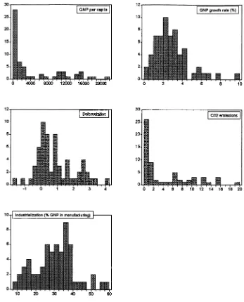
Income per capita represents consumer’s purchasing power and approximates the consumption patterns. We accompany income per capita with population density as explanatory variables to capture both scale and composition of consump-tion activities. We also consider the importance of some variables like the distribu-tion of GDP in manufacturing in order to examine the importance of specific sources of pollution in the analysis. We also take into consideration some other socio-economic variables to see their influence in this kind of analysis. Finally,
dealing with the long-run character of CO emissions we include in the regressors2
the growth rate of the economies of the countries under examination.
Thus, we have used the following variables: GDP per capita in purchasing power
Ž . Ž .
parity million $, 1991 ; the average annual growth rate % of GDP in 1980᎐1991;
Ž . Ž
population density 1993, per 1000 hectares ; infant mortality rate per 1000 live
. Ž .
births in 1990᎐1995 ; urban population % of total, 1995 ; distribution of GDP in
Ž . Ž .
manufacturing %, 1991 ; deforestation average % change, 1980᎐1990 ; and CO2
Ž .
per capita emissions in tons . The source of the last variable is Rodenburg et al.
Ž1995 while the rest of the variables were obtained from World Resources WRI,. Ž
.
1991, 1994 . Frequency distributions for the main variables of the study are
reported in Fig. 1.3
6. Discussion of results
6.1. Separating hyperplane model
6.1.1. Magnitudes of 1 and 2y1
Ž .
In the deforestation model estimates of1arey0.429 andy0.469 see Table 1
for the normal and Student’s t, respectively, i.e. higher GNPrc leads to lower
deforestation. The estimate of 2y1 is not statistically significant thus the two
3
Fig. 1. Frequency distributions for main variables of the study.
regimes are not different in terms of coefficients. In the CO model the estimates2
of 1 are 1.078 and 0.992, respectively. Again 2y1 is not significant. This can
be seen also from 95% Bayes probability intervals for ␥5. They are, generally, very
dispersed and do include the origin.We conclude that the two regimes do not differ in
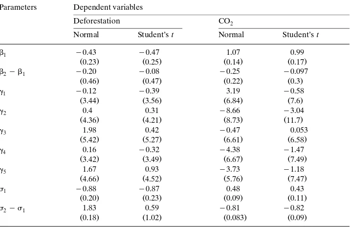
Table 1
a
Posterior results for the SHSR
Parameters Dependent variables
Deforestation CO2
Normal Student’st Normal Student’st
1 y0.43 y0.47 1.07 0.99
Notes. Student’s thas 1 d.f. i.e.s1 . Posterior standard deviations in parentheses.
6.1.2. Magnitudes of 1 and2y1
In the deforestation case the difference 2y1 is 1.833 and 0.592 for the
normal and Student’s t models with S.E.s 0.175 and 1.016. Thus according to the
normal specification 1/2 but not according to the Student’s t specification. In
the CO model the variance differences are2 y0.807 and y0.815 with S.E.s 0.083
and 0.086, respectively, i.e. highly significant. Thus we may conclude that the two
regimes differ in terms of error¨ariances of the en¨ironmental degradation equation.
This means that the variances of deforestation or CO equations are different2
and therefore policy changes, which affect GNP will not have the same result in high-income and low-income countries because of the different variances. When
we use CO2 as the dependent variable we find that 1)2 so low-income
countries have higher dispersion. Therefore policy measures which increase GNP
will decrease CO emissions with higher certainty in high-income countries. The2
opposite is true if we use deforestation as a dependent variable.
( )
6.1.3. Magnitudes of␥1. . .␥5 separating hyperplane coefficients
As can be seen from their posterior means and posterior standard errors noneof
Ž .
the regressors urbanization, industrialization, mortality, growth or GNP appears
Ž
to be a separator. The sign of ␥5 the coefficient of GNP in the separating
.
hyperplane is positive when we consider the deforestation equation and negative
cases. In this sense there is no e¨idence to support separation according to GNP or other economic and demographic¨ariables, which implies no support for an EKC.
6.1.4. Discussion of country membership to regimes
We found that the two regimes are different in terms of 12 although this cannot
be explained by economic and demographic variables. Due to the fact that
estimates of ␥i appear to be insignificant, allocating countries to the two regimes
according to the separating hyperplane should be viewed with conservatism. However, it is useful to compare separation probabilities across models and across dependent variables.
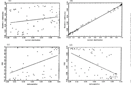
6.1.5. Discussion of differences between normal and Student’s t specifications
Fig. 2a,b presents graphs of the probability of regime 2 for the Student’s t vs. the
normal specification, using deforestation and CO as dependent variables, respec-2
tively. Fig. 2c,d plots the same probability for CO2 vs. deforestation for the
Student’s t and normal distributions, respectively. From Fig. 2a,b, we see that
Student’s t and normal distributions give comparable results only for CO . For2
deforestation, there is significant disagreement in the separation probabilities ᎏ
although they tend to be positively correlated, and strongly so under the Student’s t
specification.
Fig. 2c,d reveals significant divergence in the separation properties of different
Ž .
dependent variables. Under a normal specification Fig. 2c probabilities of regime
2 for CO and deforestation, show significant scattering around their regression2
line. Under a Student’s t specification not only that happens but they also tend to
be negatively correlated. Therefore it seems that not only the choice of dependent variable, but also the stochastic specification of switching regression models, affects
separation significantly according to environmental degradation and economic᎐
demographic factors. Thus applied researchers who venture into testing for the existence of an EKC, should not only examine alternative dependent variables and alternative sets of regressors, but they should also examine different stochastic specifications for their switching regime or linear regression models. This adds another dimension of model uncertainty, yet it is necessary practice because EKCs are sensitive to all these factors. To put things in a different manner, given the
choice of dependent and explanatory variables, EKCswill be sensiti¨eto alternative
distributional assumptions about the error term.4 In cross-sectional studies, this is
something that applied researchers should expect, and therefore they should properly account for it in order to avoid excess sensitivity of results to the nature of the disturbance term.
6.2. Exogenous break model
The most striking result that emerges from the exogenous break model is our
4
()
Halkos,
E.G.
Tsionas
r
Energy
Economics
23
2001
191
᎐
210
205
Ž . Ž . Ž . Ž .
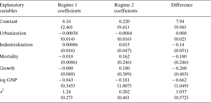
Table 2
a
Ž .
Posterior results for the EBSR dependent variable: deforestation
Explanatory Regime 1 Regime 2 Difference
variables coefficients coefficients
Constant 8.16 0.220 7.94
Ž2.40. Ž9.81. Ž9.98.
Urbanization y0.00038 y0.0084 0.008
Ž0.014. Ž0.016. Ž0.02.
Industrialization 0.00086 0.015 y0.14
Ž0.016. Ž0.047. Ž0.051.
Mortality y0.018 0.162 y0.180
Ž0.0086. Ž0.246. Ž0.246.
Growth y0.080 0.180 y0.260
Ž0.088. Ž0.389. Ž0.403.
Posterior standard deviations in parentheses.
failure to find a posterior mean for the break zU significantly lower than the
Ž . U
maximum value of z i.e. log GNPrc in our specification . Estimates of z are
9.418 and 9.453 with posterior S.E.s 0.572 and 0.430 for deforestation and CO2
equations, respectively. These are approximately 94% of the maximum value of log
GNPrc. Moreover, the differences of 1iy2i appear to be insignificant. The
2 2 Ž
same is true for the difference 2y1 estimates are 1.037 and 0.217 with S.E.s
.
0.572 and 0.43, respectively ᎏ see Tables 2 and 3 . Thus,we find no e¨idence for a
structural break from log GNPrc.
For the deforestation model, mortality rates and log GNPrc are significant in
the first regime but none of the variables is statistically significant in the second
regime. For the CO model only industrialization and log GNP2 rc are significant in
the first regime. Notice that higher GNP implies lower deforestation in the first
regime but higher CO2 emissions. We conclude that measuring en¨ironmental
degradation using deforestation or CO makes a difference.2
Only for the deforestation model we find that 22y12 is close to significance
Ž1.037 and with S.E. 0.572 . So it turns out that we find very little evidence to.
support the existence of two regimes with differences in coefficients andror error
variances.
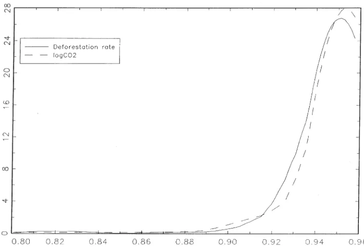
6.2.1. Marginal posterior distribution of zU
Marginal posterior distributions of zU for the deforestation and CO model are2
shown in Fig. 3. From inspection it follows that the mass is concentrated between
Table 3
a
Ž .
Posterior results for the EBSR dependent variable: CO2
Explanatory Regime 1 Regime 2 Difference
variables coefficients coefficients
Constant y6.23 6.02 y12.25
Ž1.34. Ž14.33. Ž14.31.
Urbanization 0.0063 0.0076 y0.0013
Ž0.007. Ž0.0203. Ž0.0217.
Industrialization 0.025 y0.022 0.048
Ž0.009. Ž0.045. Ž0.045.
Mortality y0.0057 0.362 y0.368
Ž0.0049. Ž0.278. Ž0.28.
Growth 0.0448 0.434 y0.389
Ž0.050. Ž0.365. Ž0.369.
log GNP 0.771 y0.731 1.502
Ž0.185. Ž1.468. Ž1.467.
2
0.406 0.188 0.217
Ž0.09. Ž0.418. Ž0.430.
a
Posterior standard deviations in parentheses.
both the log CO and deforestation models these distributions are approximately2
the same.
Ž .
7. Concluding remarks
In this paper we tested empirically the existence of an EKC using switching regime models and Bayesian Markov chain Monte Carlo methods. The evidence indicates that higher GNP per capita leads to lower deforestation. A monotonic relationship exists between environmental degradation and income because economic growth does reduce deforestation and therefore in that sense there is an EKC. The measurement of environmental deterioration using deforestation or
CO does make a difference. Additionally, we find that the demographic and2
economic variables considered here could not explain the difference between low and high damage countries.
Our main conclusions were that the two regimes do not differ in terms of their parameters. They do differ in terms of error variances at the environmental degradation equations and there is no evidence to support separation according to GNP or other economic and demographic variables which does not provide support for an inverted-U-shaped EKC.
The rejection of the EKC implies that we may not have a certain environmental degradation along a nation’s development route. Economic growth appears to improve environmental quality in developing countries and so policies to stimulate growth are recommended. There is empirical evidence that trade liberalization is positively correlated with growth. To that extent our evidence supports the view that higher rate of liberalization is associated with low degradation.
Acknowledgements
The paper benefited from the comments of an anonymous referee.
References
Albert, J., Chib, S., 1993. Bayes inference via Gibbs sampling of autoregressive time series subject to Markov mean and variance shifts. J. Bus. Econ. Stat. 11, 1᎐15.
Ansuategi, A., Barbier, E.B., Perrings, C.A., 1998. The environmental Kuznets curve. In: Van den
Ž .
Bergh, J.C.J.M., Hofkes, M.W. Eds. , Theory and Implementation of Economic Models for Sustainable Development. Kluwer.
Arrow, K., Bolin, B., Costanza, R. et al., 1995. Economic growth, carrying capacity and the environment. Science 268, 520᎐521.
Cole, M.A., Rayner, A.J., Bates, J.M., 1997. The environmental Kuznets curve: an empirical analysis. Environ. Dev. 2, 401᎐416.
Cropper, M., Griffiths, C., 1994. The interaction of pollution growth and environmental quality. Am. Econ. Rev. 84, 250᎐254.
Ž .
Dijkgraaf, E., Vollebergh, H.R.J., 1998. Growth andror ? environment: is there a Kuznets curve for carbon emissions? Paper presented at the 2nd biennial meeting of the European Society for Ecological Economics, Geneva, 4᎐7 March 1998.
Ekins, P., 1997. The Kuznets curve for the environment and economic growth: examining the evidence. Environ. Planning A 29, 805᎐830.
Ž
Gelman, A., Rubin, D.B., 1992. Inference from iterative simulation using multiple sequences with
.
discussion . Stat. Sci. 7, 457᎐511.
Geweke, J., Terui, N., 1993. Bayesian threshold autoregressive models for nonlinear time series. J. Time Ser. Anal. 14, 441.
Geyer, C.J., 1992. Practical Markov chain Monte Carlo. Stat. Sci. 7, 473᎐482.
Grossman, G., Krueger, A., 1992. Environmental impacts of a North American Free Trade Agreement. NBER Working Paper 3914. National Bureau of Economic Research, Cambridge, MA.
Grossman, G., Krueger, A., 1995. Economic growth and the environment. Q. J. Econ. 110, 353᎐377. Hamilton, J.D., 1989. A new approach to the economic analysis of non-stationary time series and the
business cycle. Econometrica 57, 357᎐384.
Hamilton, J.D., 1994. Time Series Analysis. Princeton University Press, Princeton.
Hastings, WX, 1970. Monte Carlo sampling methods using Markov chains and their applications. Biometrica 57, 97᎐109.
Holtz-Eakin, D., Selten, T.M., 1995. Stoking the fires? CO emissions and economic growth. J. Public2
Econ. 57, 85᎐101.
IBRD, 1992. World Development Report 1992. Oxford University Press, New York. Kahn, M.E., 1998. A household level environmental Kuznets curve. Econ. Lett. 59, 269᎐273.
Kaufmann, R.K., Davidsottir, B., Garnham, S., Pauly, P., 1997. The determinants of atmospheric SO2
concentrations: reconsidering the environmental Kuznets curve. Ecol. Econ. 25, 209᎐220. Kuznets, S., 1965. Economic Growth and Structural Change. New York.
Kuznets, S., 1966. Modern Economic Growth. Yale University Press.
Matyas, L., Konya, L., Macquaries, L., 1998. The Kuznets U-curve hypothesis: some panel data evidence. Appl. Econ. Lett. 5, 693᎐697.
Metropolis, N., Rosenbluth, A.W., Rosenbluth, M.N., Teller, A.H, Teller, E., 1953. Equations of state calculations by fast computing machines. J. Chem. Phys. 21, 1087᎐1091.
Muller, R, West, M., McEachern, S., 1997. Bayesian models for non-linear autoregressions. J. Time Ser. Anal. 18, 593᎐614.
Panayotou, T., 1993. Empirical tests and policy analysis of environmental degradation at different stages of economic development. Working Paper WP238. Technology and Employment Programme, International Labor Office, Geneva.
Panayotou, T., 1995. Environmental degradation at different stages of economic development. In:
Ž .
Ahmed, I., Doeleman, J.A. Eds. , Beyond Rio: the Environmental Crisis and Sustainable Liveli-hoods in the Third World. MacMillan, London.
Pezzey, J.C.V., 1989. Economic analysis of sustainable growth and sustainable development. Environ-ment DepartEnviron-ment Working Paper No. 15. The World Bank, Washington, DC.
Ritter, C., Tanner, M.A., 1992. Facilitating the Gibbs sampler: the Gibbs stopper and the griddy-Gibbs sampler. J. Am. Stat. Assoc. 87, 861᎐868.
Rodenburg, E., Tunstall, D., van Bolhuis, F., 1995. Environmental indicators for global cooperation. The World Bank, Working Paper No. 11. UNEP Global Environmental Facility.
Schmalensee, R., Stoker, T.M., Judson, R.A., 1995. World Energy Consumption and Carbon Dioxide Emissions: 1950᎐2050. Sloan School of Management, Massachusetts Institute of Technology, Cam-bridge, MA.
Selten, T., Song, D., 1994. Environmental quality and development: is there a Kuznets curve for air pollution emissions? J. Environ. Econ. Manage. 27, 147᎐162.
Shafik, N., 1994. Economic development and environmental quality: an econometric analysis. Oxford Econ. Pap. 46, 757᎐773.
Shafik, N., Bandyopadhyay, S., 1992. Economic growth and environmental quality: time series and cross-country evidence. Background paper for the World Development Report 1992. The World Bank, Washington, DC.
Stern, D.I., 1998. Progress on the environmental Kuznets curve? Environ. Dev. 3, 175᎐198.
sulfur? Working Paper in Ecological Economics 9804, Centre for Resource and Environmental Studies, Australian National University, Canberra.
Ž
Tanner, M.A., Wong, W.H., 1987. The calculation of posterior distributions by data augmentation with
.
discussion . J. Am. Stat. Assoc. 82, 528᎐550.
Ž .
Tierney, L., 1994. Markov chains for exploring posterior distributions with discussion . Ann. Stat. 22, 1701᎐1762.
Tsionas, E.G., 1999. Monte Carlo inference in econometric models with symmetric stable disturbances. J. Econometrics 88, 365᎐401.
UNDP, 1992. Human Development Report 1992. Oxford University Press, New York.
Wang, P., Bohara, A.K., Berrens, R.P., Gawande, K., 1998. A risk-based environmental Kuznets curve for hazardous waste sites. Appl. Econ. Lett. 5, 761᎐763.
WRI, 1991. World Resources 1990᎐91. World Resources Institute, Washington, DC. WRI, 1994. World Resources 1994᎐95. World Resources Institute, Washington, DC.