chapter 6 pivot tables modul dss

(1)

Handaru Jati, Ph.D

Universitas Negeri Yogyakarta

(2)

Chapter Overview

6.1 Introduction

6.2 Pivot Tables

6.2.1 Terminology

6.2.2 Creating a Pivot Table

6.3 Further Modifications

6.3.1 Pivot Table Toolbar and Options

6.3.2 Grouping

6.3.3 Calculated Fields and Items

6.3.4 GETPIVOTDATA Function

6.4 Pivot Charts

6.5 Summary

6.6 Exercises

Chapter 6

(3)

6.1 Introduction

This chapter instructs the reader on how to create pivot tables and pivot charts. We have found that even experienced Excel users are not familiar with the benefits of using these tools. Pivot tables and pivot charts are a great tool for organizing large amounts of data in a format which is clearer for the user to understand. They can be useful tools for displaying large amounts of output to a user in a DSS application. For example, in Part III of this book, we describe a Supply Chain Management DSS in which we use several pivot tables and pivot charts to present the output of the application to the user. We will also discuss how to create pivot tables and pivot charts using VBA in Chapter 21.

6.2 Pivot Tables

Pivot tables are used to transform large amounts of data from a table or database into an organized summary report. The word “pivot” refers to the ability to rotate and reorganize the row and column headings from an original database into a new table. We will now explain the parts of a pivot table and show you how to create one.

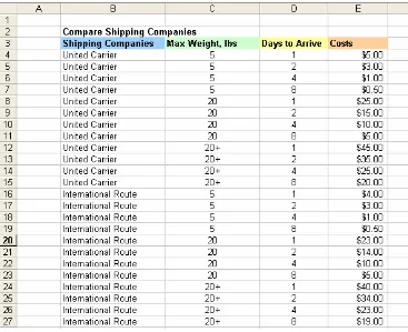
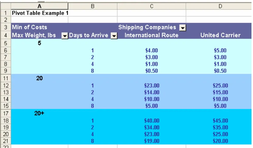
The table in Figure 6.1 contains the “Costs” for varying “Maximum Weights” and the number of “Days to Arrive” for two different “Shipping Companies.” Suppose that an employee is assigned the task of comparing the performance of these shipping companies and presenting the results to his manager. The employee wants to summarize this data so that a clear comparison can be made between the “Cost” values of each company. We can observe in this table that there are three common values of “Max Weight” (5, 20 and 20+) and four common values for “Days to Arrive” (1, 2, 4 and

(4)

Chapter 6: Pivot Tables 3

Figure 6.1 The above data can be used in a comparative experiment, but would be better organized with a pivot table.

(5)

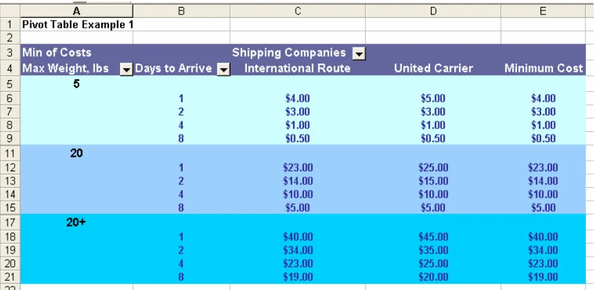
Figure 6.2 The final pivot table reorganizes the data so that costs can be easily compared.

6.1.1

Terminology

In this table, “Max Weight” and “Days to Arrive” are referred to as Row Fields; each value in the fields from Figure 6.1 is shown as a row in the pivot table (Figure 6.2). “Shipping Companies” is a Column Field, since its values serve as column headings in the pivot table. The “Cost” values that appear in cells C6:E21 compose the Data Field

that is used to create the pivot table. The Page Field, a larger category that can group all of the data in the table, would be seen at the top of the worksheet. While we have not selected a page field for this table, an example like “Shipping Regions” would work well.

The “Minimum Cost” column is an example of the Grand Totals feature of pivot tables, which we will discuss in more detail in a later section. Since the minimum costs are computed for each row, this is a Row Grand Total; there are also Column Grand Totals. The title of the table, “Min of Costs,” indicates that any Grand Totals would calculate minimums of the data in the Data Field. The Field Settings of the Data Field

determine these data relations. Field Settings can also be applied to Row or Column Fields to create Subtotals; we will also discuss Subtotals in more detail in a later section.

(6)

(a)

(b) Figure 6.3 The fields have drop-down lists of their corresponding values that can be

selected or deselected to change the pivot table. (a) Deselecting the value 20+ from the “Max Weight” field. (b) The updated pivot table no longer displays data for the 20+ value of “Max Weight.”

Row Field Each value, or item, in this field is shown as a row.

Column Field Values are shown as column headings.

Page Field A larger category that can group all data in the table.

Data Field The main area of the table where comparative values are shown.

Grand Totals Calculations applied to rows or columns of data in the Data Field.

(7)

6.1.2

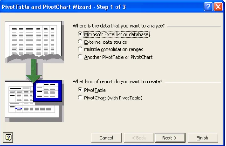
Creating a Pivot Table

Now we will explain how to create a pivot table. First, we select Data > Pivot Table and Pivot Chart Report from the menu. The window in Figure 6.4 thenappears. We need to follow three simple steps in order to create a pivot table. These are: specify the data location, specify the data, and create the table.

STEP 1: Data Location

This step, as represented in Figure 6.4, asks us to identify the location of the data that we want to analyze and the kind of report that we want to create. Excel lists four main data location options: Microsoft Excel list or database, External data source, Multiple consolidation ranges, or Another pivot table or pivot chart. The most common data location is a Microsoft Excel list or database. As in the example above, our original table is in an Excel worksheet. In the case of an External data source, the data is stored in another file or database, for example, if we are using a different program, such as Microsoft Access, to collect large amounts of data. We will discuss the use of external data in Chapter 10. The Multiple consolidation ranges option refers to data that comes from a variety of non-adjacent ranges or worksheets. The final option, Another pivot table or pivot chart, takes data from an existing pivot table, or pivot chart, and uses it to create a new one. When using pivot tables, any changes we make to the original data source will not be updated automatically in the pivot table. We have to update the pivot table manually or specify an option to update the pivot table when the workbook is opened in order to reflect the correct changes in the data.

(8)

Figure 6.4 Step 1: Specifying the location of the data and the type of report to create.

STEP 2: Data Source

In the second step, we select the data to be used in the pivot table (see Figure 6.5). If we had chosen an External data source or Another pivot table or pivot chart in Step 1,

we would use the Browse button to select our data. Again, we will discuss this in detail in Chapter 10. Because we have a Microsoft Excel list or database in this example, we can highlight the data from our worksheet that we want to use in the pivot table. From the table shown in Figure 6.1, we highlight cells B3:E27, the data cells and the column headings. The first row of the highlighted data must contain column headings. In Figure 6.5, we enter the Range as follows, where “Data-Shipping” is the name of our worksheet:

‘Data-Shipping’!$B$3$E$27

Now, we press Next to continue to Step 3.

Figure 6.5 Step 2: Selecting the actual data by highlighting a range of cells or choosing a file with the Browse option.

(9)

The third and most important step, shown in Figure 6.6, has three sub-steps. These steps allow us to specify exactly how we want to reorganize our data in the new table. The first sub-step, in the middle of the screen in Figure 6.6, designates the location of the new pivot table. This option allows us to place the pivot table in a new worksheet or in a particular area of the current worksheet. For this example, we have chosen to put our pivot table in a new worksheet.

Figure 6.6 Step 3: Specifying the location of the pivot table and working with Layout and Options features.

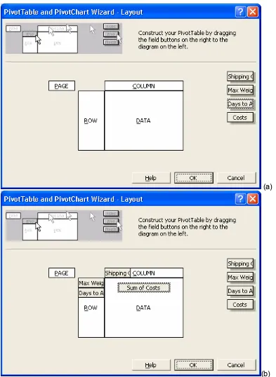
The next sub-step, activated by pressing the Layout button, allows us to select our layout. The Layout sub-step, detailed in Figure 6.7(a), allows us to organize our data by determining which column heading from the original data we want to become a Row,

Column, Data, or Page Field. We select one of our field names from the right-hand side of the window and drag it to one of the layout areas corresponding to the different field types. Because we want “Max Weight” to be a Row Field, we click and drag it to the Row

layout area. We click on “Days to Arrive” and drag it to the same layout area since we also want it to be a Row Field. We then click on “Shipping Companies” and drag it to the

(10)

(a)

(b)

Figure 6.7 Layout sub-step: Click and dragging field names to the layout area shown in the center of the window, which will determine which fields become Row Fields, Column Fields, and the Data Area. It is also possible to specify a Page Field.

(11)

technique in a later section. The third sub-step, Options, which we explore in a later section, allows us to manipulate various features of the pivot table. Now, we click the

Finish button to display the completed pivot table, presented in Figure 6.8.

Figure 6.8 The final pivot table after specifying the source data and layout.

Now that we have created the pivot table, we can use the drop-down buttons to search for specific data. We will discuss further data searching and manipulation in the next section.

6.2 Further Modifications

(12)

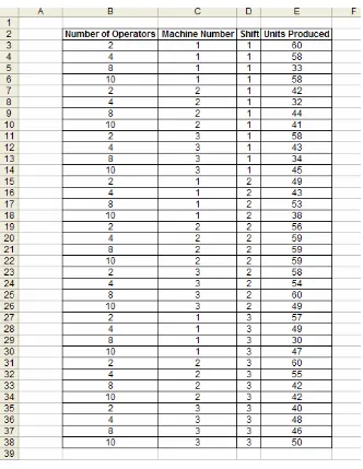
Figure 6.9 This table records “Units Produced” for various combinations of operators, machines, and shifts.

(13)

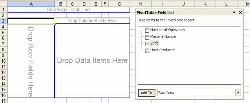
Figure 6.10 Setting the Row Fields, Column Fields, and Data Field in the spreadsheet using the Pivot Table Field List.

Figure 6.11 The completed pivot table.

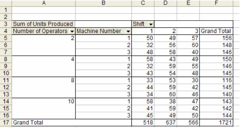
The pivot table analyzes the set of data included in the Data Field and the Field Setting

for the table manipulates the presentation of this data. In the table created in the above example, the default Field Setting applied to the “Units Produced” data field is Sum, which can be noted by the “Sum of Units Produced” title automatically given to the table (see Figure 6.11). Any Grand Totals or Sub Totals calculated would show sums of the “Units Produced” values in relative row fields or column fields. We can use the Options

setting of the pivot table to show or hide these Grand Totals.

(14)

Figure 6.12 Row and column Grand Totals show the sums of “Units Produced.”

There are other Field Setting options aside from Sum (as we saw in the first example with shipping data when showing “Minimum Costs”). To look at these, we double-click on the “Sum of Units Produced” title, or we can select a cell in the Data Field and use the

Pivot Table Toolbar, which we will discuss later. The dialog box shown in Figure 6.13 then appears.

Figure 6.13 Field Settings for the “Units Produced” Data Field.

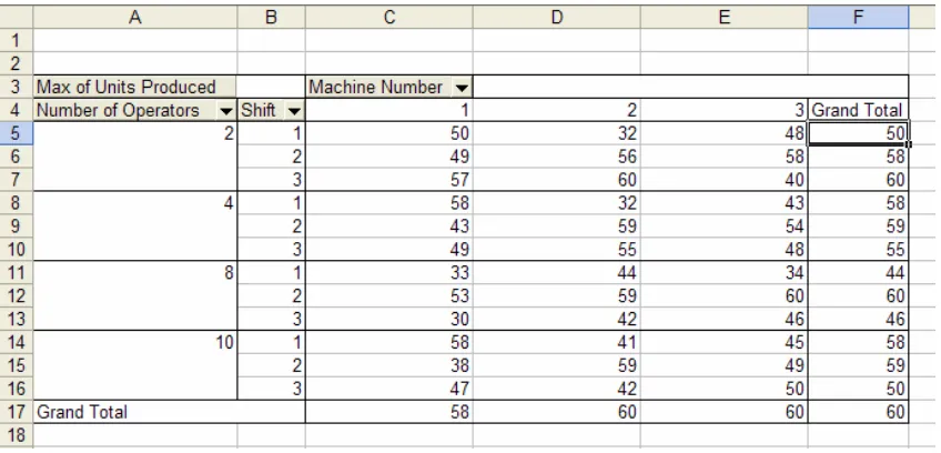
We can select any of the preset calculations in the Summarize by window. For example, we can choose Max to better analyze the combination of operators, machines, and shifts that produces the most units (see Figure 6.14). With Max, we can clearly see the combination of “Number of Operators” and “Machine Number” that produces the most units during any “Shift.” Any Grand Totals or Subtotals now display the maximum values of “Units Produced.” The Name value should automatically update depending on the summary chosen; this name can also be changed manually. Clicking on the Number

(15)

Figure 6.14 The Field Setting on the “Units Produced” Data Field has now been changed to Max. All Grand Totals have been updated.

We can use the Options button to modify the data further after the main summarizing has been completed. For example, we can choose to show the data as a percentage of a given set of field values (see Figure 6.15).

Figure 6.15 The Options button allows a user to further modify data from a selected field.

(16)

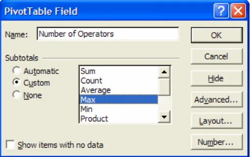
Row Fields. For example, to perceive the total number of “Units Produced” for each “Number of Operators” or for each “Machine Number,” we add Subtotals to either of these fields. To do so, we simply click in one of these fields and then select the Field Settings option, either by right-clicking in the field or from the Pivot Table Toolbar, which we will discuss later. The window in Figure 6.16 then appears. This window resembles Figure 6.13, which allows users to modify Field Settings for Data Fields. Again, we can choose from the list of preset summarizing, or subtotaling, options in the central window.

Figure 6.16 Using Field Settings for Row Fields to create Subtotals.

In this PivotTable Field dialog box, we have selected the Max subtotal option to add

Subtotals for the “Number of Operators” Row Field. The Pivot Table then summarizes the maximum number of “Units Produced” for each “Number of Operators” value in separate rows (see Figure 6.17). This option also adds Max Subtotals for the “Machine Number” Row Field, which are summarized at the bottom of the table. Calculating these

(17)

Figure 6.17 Adding Subtotals for the “Number of Operators” and “Machine Number” Row Fields to the pivot table.

6.2.1

Pivot Table Toolbar and Options

With the Pivot Table Toolbar, we can easily modify the pivot table after it has been created. This toolbar features icons (see Figure 6.18) as well as a drop-down list of options (see Figure 6.19). We can also access several of these options by right-clicking in any field of the pivot table. Note that we must select a cell in the pivot table in order to activate the Pivot Table Toolbar.

(18)

Figure 6.19 The list of drop-down options available from the Pivot Table Toolbar.

We will discuss eleven of the main Toolbar Options, giving a brief description of each in the following order: Format Report, Pivot Chart, Hide/Show Details, Refresh, Field Settings, Pivot Table Fields List, Wizard (and Layout), Grouping, Formulas (or

Calculated Fields and Items), and Table Options. The order of these options correlates with their location on the toolbar.

(19)

Figure 6.20 Adding more options to the Pivot Table Toolbar.

(20)

Figure 6.21 The first icon on the pivot table toolbar, Format Report, allows a user to select a report style for a table.

(21)

The next item is Pivot Charts. We will actually discuss this icon in a later section, but, for now, note that we can create a Pivot Chart directly from the Pivot Table with the toolbar or by right-clicking on the table.

The next two icons on the Pivot Table Toolbar, Hide Detail and Show Detail, are simply visual preferences that allow us to hide or view all related values for a selected item. We can also double-click on any item in a field to hide or view related data.

The next icon is the Refresh option, , which updates the data shown in our pivot table if we change our source data. For example, if we update the “Units Produced” data for 2 operators on all machines in Shift 1 in the original table, clicking the refresh icon reflects this change in the pivot table (see Figure 6.23). In the figure, the data values are updated and any Grand Totals or Subtotals are recalculated.

(22)

(b)

Figure 6.23 (a) The data in the original table is changed. (b) The refresh button reflects these changes in the pivot table.

We have already described the next icon, which is used to modify Field Settings, in the previous section.

The subsequent icon shows the Pivot Table Fields List, which creates the layout of the pivot table if Step 3’s Layout sub-step of the Wizard is not used. We simply select a field name from the list and drag it to the table. To remove a field from the table, we click on the field title in the table and drag it outside of the table. It is also helpful to observe all fields available from the original data if some fields are hidden in the pivot table. If we do

not wish to modify the layout using the Pivot Table Fields List, we can choose the icon (or Wizard from the list of Pivot Table drop-down options) to return to Step 3 of the

(23)

Figure 6.24 The pivot table is updated to reflect the new layout. We have switched the “Machine Number” and “Shift” fields.

The next two items to discuss are Grouping and Formulas, both of which can be found in the Pivot Table drop-down list in the toolbar. We discuss Grouping in the following section and Formulas, or Calculated Fields and Items, in the section after.

To work with pivot table options, we choose Table Options from the Pivot Table drop-down list in the toolbar. The window in Figure 6.25 then appears. We can also access the Options window by right-clicking on the pivot table, if it has already been created, and choosing Table options from the drop-down list. Remember that this is also a sub-step of Step 3 of the Wizard. This table provides a variety of options, beginning with the option to enter a name for the pivot table in the text area next to Name at the top of the window. Besides Name, this table contains two main categories: Format options and

Data options.

Under Format options, we can edit some of the details of the table. The first two options allow us to display Grand Totals for our columns or rows. Another formatting option,

Page layout, features a drop-down list that allows us to alter our data display. In Figure 6.25, we have selected the default option of Down, then Over. Below that option, we can specify how many fields should appear in a column; the default value is zero. Next, we can choose to replace empty or erroneous cells with specific text or symbols. These features are easy to experiment with.

(24)

Figure 6.25 Options Step: Select Format and Data options to fine-tune a final pivot table’s appearance and features.

6.2.2

Grouping

Grouping items in a Row or Column Field allows us to further manipulate how we view or search for data in a pivot table. To group field values, we select the field and choose

(25)

Figure 6.26 Applying grouping to the values of the “Number of Operators” Row Field.

The Grouping window in Figure 6.27 then appears. In this window, we specify the intervals that we want to create. Here, we designate 2 and 10 as our starting and ending values, and set an interval of 4 operators. The updated pivot table is shown in Figure 6.28.

(26)

Figure 6.28 The updated pivot table now shows the values for “Number of Operators” as intervals.

We can ungroup any field by selecting Group and Show Detail and Ungroup Data.

6.2.3

Calculated Fields and Items

To create a Calculated Field or Calculated Item, we click on Pivot Table > Formulas > Calculated Field (or Calculated Item) in the toolbar drop-down options. The window in Figure 6.29 then appears. Here, we can name and define a formula associated with the creation of a new field or item. This formula is stored with the pivot table. Unlike Grand Totals or Subtotals, we can enter any formula to be applied to the values in the selected field, and a new field will then be created.

(27)

Figure 6.29 Entering a formula to create a new calculated field.

A new data field called “Variable Cost” has been added to the pivot table in Figure 6.30. Also note that there is now a drop-down arrow for “Data” at the top of the table; it allows us to select a set of data fields to show. That is, we could now hide “Max of Units Produced” and show “Variable Cost” only.

Figure 6.30 Adding a new Calculated Field to the pivot table.

Calculated Items create a single row rather than an entire new column of data. First we select a Row Field, and then we go to Pivot Table > Formulas > Calculated Item from

Pivot Table Toolbar.

Calculated Field or Calculated Item

(28)

6.2.4

GETPIVOTDATA Function

The GETPIVOTDATA function extracts a particular set of data-based values specified for each Row and Column Field. The format of this function is:

=GETPIVOTDATA(desired_field, range_of_desired_data, field1, item1, …)

The desired_field is the field that contains the value we are searching for. The range_of_desired_data is the range in the pivot table that contains this field. The remaining field and item values allow us to refine our search if desired. The field and item values can be listed in any order, regardless of the pivot table layout.

For example, suppose we want to find the number of units produced during Shift 2 on Machine 2 when 8 operators are working. We type the following in a cell on the worksheet:

=GETPIVOTDATA(“Units Produced”, C5:E19, “Shift”, 2, “Machine Number”, 2, “Number of Operators”, 8)

The value for this search is 59 units produced (see Figure 6.31). GETPIVOTDATA can be a very useful function when pivot tables are involved in a large spreadsheet with other applications. That is, this function can be used on a “Report” sheet that refers to information searched from a pivot table. It can also be useful when a user interface is created, as we will see in applying VBA.

(29)

6.3 Pivot Charts

We can additionally create a chart that shows the data we have selected in our pivot table. To do so, we click on the second icon in the pivot table toolbar, choose from the

Pivot Tables drop-down options, or right-click on the table. This automatically creates a new worksheet with a chart of our pivot table (see Figure 6.32). We call this chart, which is created from a pivot table instead of directly from the original source data, a Pivot Chart. Remember, we can also create a Pivot Chart by highlighting the source data, choosing Data > Pivot Table and Pivot Chart Report from the menu and selecting Pivot Chart from the options in Step 1.

We can see the different times for each layout in a bar above the corresponding job type and run number. Note the field names “Number of Operators” and “Machine Number”at the bottom of the chart. We can select these fields to vary the items displayed. Assume we only want to view the “Units Produced” on Machine 3. We select the field “Machine Number”and unclick the numbers 1 and 2 (see Figure 6.33). Any change in viewing field items made to the chart is reflected in the pivot table, and likewise, any changes to the viewing field items in the pivot table are reflected in the chart. These options are useful when presenting or analyzing data.

(30)

Figure 6.33 Thechart is updated to show the units produced on Machine 3 only.

If we do not like the Pivot Chart format created by Excel, we can modify the Chart Type using the same techniques described in Chapter 5. That is, we can right-click on the chart and select Chart Type from the list of options (see Figure 6.34). With this list of drop-down options, we can also modify other chart details, such as formatting. To do so, we have to make sure that we link the Source Data to the pivot table so we can transfer the filtering capabilities to the pivot chart.

(31)

6.4 Summary

¾ Pivot tables transform large amounts of data from a table or database into an organized summary report.

¾ The three steps to create a pivot table are: Specify Location, Select Data, and Create Table Layout with specified options.

¾ From categories in your original table, select Row and Column Fields to group your data. You also choose a Data Area of comparative values. A Page Field can be created to organize your entire table by different overall categories.

¾ Toolbar options include: Format Report, Pivot Chart, Hide/Show Details, Refresh, Field Settings, Pivot Table Fields List, Wizard (and Layout), Grouping, Formulas (or Calculated Fields and Items), and Table Options.

¾ Use Grouping to create intervals in field values.

¾ You can create Calculated Fields or Calculated Items to further analyze the data in your table. Some common formulas already constructed by Excel include SUM, MIN, and MAX. Grand Totals and Subtotals use the SUM formula to display these calculations of your row or column data.

¾ GETPIVOTDATA searches for data in a pivot table using field value criteria. ¾ Pivot Charts use pivot tables as their Source Data so that filtering options are

transferred to the chart as well.

6.5 Exercises

6.5.1

Review Questions

1. What are pivot tables and how are they used?

2. What are the parts of a pivot table into which items from the original database can be placed?

3. What do the Grand Totals and Subtotals features of a pivot table do? 4. How do you begin to create a pivot table?

5. What are the three main steps in creating a pivot table?

6. What pivot table option will allow automatic updates of a pivot table when changes have been made to its data source?

7. How do you add a calculated field or item to a pivot table?

8. List four of the common pivot table fields that Excel makes available automatically.

9. What purpose do the drop-down arrows on a pivot table serve? 10. How can you apply an existing report style to a pivot table? 11. How does a pivot chart differ from a pivot table?

12. How can you create a pivot chart from the source data? 13. How do you group data?

14. Can Subtotals be created for Data Fields? How are Subtotals for Column Fields created?

15. What are the parameters of the GETPIVOTDATA function?

Pivot Chart A chart created from a pivot table or directly from the

source data using the same layout features and other options as a pivot table.

(32)

6.5.2

Hands-On Exercises

1. The “Store Chain” example on the included CD displays the location, size category, owner, and quarterly sales for each store owned by a particular store chain.

Organize this data into a pivot table. Show quarterly results using the city as the first criteria, the size second, and the owner third. Do you notice any trends in this method?

2. A furniture manufacturer has distribution centers in different regions of the country that supply retailers with goods to sell. The “Supply Chain” spreadsheet on the included CD is used to track the quantity of products from each product collection being shipped from a distribution center to a retailer. Create a pivot table that allows any member of the supply chain to determine the following factors in the given order quickly: the distribution center supplying furniture, the retail chain receiving the furniture, the location of the retailer, the product collection of the furniture, and the total quantity of furniture shipped. Format your table using an existing report style.

3. A student traveling home for the holidays is comparing flights in an effort to find a cheap flight with few connections at a desirable time. The student wishes to travel from the state of Florida to the city of Pittsburgh. There are numerous combinations of flights available to travel this route. Using the data provided in the “Fly Home” spreadsheet on the included CD, create a pivot table that will allow the student to quickly pull up flights between various cities to determine which flight or combination of flights is the most desirable. The table should also highlight the least expensive flight departing each city. Format your table using an existing report style.

4. Refer to the soft drink bottling plant introduced in Chapter 4, Problem 6. In an effort to reduce the number of nonconforming bottles, the plant manager has decided to reallocate the products it offers to the bottling lines that package those products. Before doing this, the manager must be able to compare the current costs of bottling each product. Using the data provided in the “Soft Drink” spreadsheet on the

included CD, create a pivot table that will enable the manager to perform this cost comparison based on the drink type, number of fluid ounces, and material of each bottle. Format your table using an existing report style.

5. Use your solution to the previous problem to create a pivot chart that compares the costs of bottling each product. What are the characteristics of the most expensive product to bottle?

6. The following table displays postal service rates for shipping packages. Packages can be shipped via Express, First Class, Priority, or Standard mail. Express and First Class mail may also be certified, which means that the sender can receive

(33)

Shipment Type Certification First Ounce Rate

A business frequently sends out packages that weigh approximately 10 ounces. Calculate the cost of mailing a 10-oz package via each of the means shown in the table. Create a pivot table that displays the minimum cost of sending a 10-oz package via each of the shipment types. The table should also display the overall minimum cost of mailing a 10-oz package. Finally, format your table using a report style of your own creation.

7. The owner of a campus textbook store has noticed that the store’s customers must wait in particularly long lines during the first few weeks of classes. Concerned about losing business to stores with speedier lines, the owner wants to analyze the length of the store’s queues for comparison with queues at competing stores. To do so, she measures the following values at five random times throughout the day, every day for a week: the length of the queue, the number of cashiers attending customers, and the number of idle cashiers. The “Queue” spreadsheet on the included CD contains a table of her results. Create a pivot table of the information she collected that

averages the store’s queue lengths for different times of the day and week and for different numbers of busy and idle cashiers. Apply formatting to complete your table.

8. Use the pivot table you created in the previous problem to determine which hour of the day has the highest average queue lengths. Then create a pivot chart to display the average queue lengths for that hour of the day on each different day of the week.

9. A do-it-yourself retail center sells home care products in various categories, including cleaning, gardening, and hardware. The “Home Care” spreadsheet on the included CD is used to forecast the demand of products in each of the product categories for the next four months for each of the center’s regions. Create a pivot table that totals the demand for each type and category of product for each region.

10. A swarm of locusts is infesting the Mid-Atlantic region, so the projected insecticide demand has increased. The forecasted demand (in thousands of units) is now 85 for January, 89 for February, 87 for March, and 82 for April. Record these changes in the data table on the “Home Care” spreadsheet. Then refresh the data on the pivot table to reflect these changes.

(34)

12. Students at a local community college either apply to study Business or Mathematics. Determine if the college discriminates against women in admitting students to the school of their choice. Use the information given below to create a pivot table.

(35)

14. Using the data from problem 13, create a pivot table that displays the total revenue by product for each salesperson. Use the GETPIVOTDATA function to find Danny’s vacuum sales.