Full Terms & Conditions of access and use can be found at
http://www.tandfonline.com/action/journalInformation?journalCode=ubes20
Download by: [Universitas Maritim Raja Ali Haji], [UNIVERSITAS MARITIM RAJA ALI HAJI
TANJUNGPINANG, KEPULAUAN RIAU] Date: 11 January 2016, At: 20:32
Journal of Business & Economic Statistics
ISSN: 0735-0015 (Print) 1537-2707 (Online) Journal homepage: http://www.tandfonline.com/loi/ubes20
Consistent Nonparametric Tests for Lorenz
Dominance
Garry F. Barrett, Stephen G. Donald & Debopam Bhattacharya
To cite this article: Garry F. Barrett, Stephen G. Donald & Debopam Bhattacharya (2014) Consistent Nonparametric Tests for Lorenz Dominance, Journal of Business & Economic Statistics, 32:1, 1-13, DOI: 10.1080/07350015.2013.834262
To link to this article: http://dx.doi.org/10.1080/07350015.2013.834262
Accepted author version posted online: 06 Sep 2013.
Submit your article to this journal
Article views: 412
View related articles
Consistent Nonparametric Tests
for Lorenz Dominance
Garry F. B
ARRETTSchool of Economics, University of Sydney, Sydney, NSW 2006 ([email protected])
Stephen G. D
ONALDDepartment of Economics, University of Texas at Austin, Austin, TX 78712 ([email protected])
Debopam B
HATTACHARYADepartment of Economics, University of Oxford, Oxford, OX1 3UQ, UK ([email protected])
This article proposes consistent nonparametric methods for testing the null hypothesis of Lorenz dom-inance. The methods are based on a class of statistical functionals defined over the difference between the Lorenz curves for two samples of welfare-related variables. We present two specific test statistics belonging to the general class and derive their asymptotic properties. As the limiting distributions of the test statistics are nonstandard, we propose and justify bootstrap methods of inference. We provide methods appropriate for case where the two samples are independent as well as the case where the two samples represent different measures of welfare for one set of individuals. The small sample performance of the two tests is examined and compared in the context of a Monte Carlo study and an empirical analysis of income and consumption inequality.
KEY WORDS: Bootstrap simulation; Test consistency.
1. INTRODUCTION
A fundamental tool for the analysis of economic inequality is the Lorenz curve that graphs the cumulative proportion of total income, or other measure of individual welfare, by cumulative proportion of the population after ordering from poorest to rich-est. The related concept of Lorenz dominance provides a partial ordering of income distributions based on minimal normative criteria. Distribution A weakly Lorenz dominates Distribution B if the Lorenz curve for A is nowhere below that for B. As shown by Atkinson (1970), Lorenz dominance translates into simple facts concerning the degree of egalitarianism in the respective income distributions. Lorenz dominance is equivalent to the ranking of income distributions based on the class of scale-free inequality indices that respect the “principle of transfers”— whereby a progressive transfer is associated with a decrease in inequality—while avoiding the imposition of stronger addi-tional normative criteria embodied in a specific scalar index of inequality. An empirical method for directly inferring Lorenz dominance is therefore very desirable.
The work by Beach and Davidson (1983) represented a key development in the use of Lorenz curves for statistical inference in economics. They derived the sampling properties of a subset of ordinates from the empirical Lorenz curve and presented a test for the null hypothesis that two independent Lorenz curves are equal. Note that this was a test of Lorenz equality, rather than dominance, at a fixed set of population proportions. Bishop, Formby, and Smith (1991a,b) proposed a test of Lorenz dominance based on multiple pair-wise comparisons of empirical Lorenz ordinates. Davies, Green, and Paarsch (1998), Dardanoni and Forcina (1999), and Davidson and Duclos (2000) presented tests for Lorenz dominance based on a predetermined grid of points. The null hypothesis of dominance
across those fixed points imply a series of inequality restrictions that can be tested using the methods by Wolak (1989). Although these tests use information on the covariances among the set of estimated Lorenz ordinates, making them more powerful than the tests by Bishop, Formby, and Smith (1991a,b), these methods are also potentially inconsistent. By limiting attention to a small fixed set of grid points, the tests do not take account of the full set of restrictions implied by Lorenz dominance.
The aim of the current article is to develop consistent tests for Lorenz dominance. Our approach to testing is based on a class of statistical functionals defined over the difference between two Lorenz curves. A test of Lorenz dominance may be considered as a scalar measure of the extent to which one Lorenz curve (here-after LC) is everywhere above the other. Two test statistics based on specific functionals from the general class are examined in detail. The first test statistic is based on the largest difference be-tween the two LCs, a supremum or Kolmogorov-Smirnov (KS) type test, while the second is a Cramer von-Mises (CVM) type test based on the integral of the difference between the curves over the range of ordinates for which one lies above the other. This second test statistic was first presented by Bhattacharya (2007) in the context of analyzing inequality using stratified and clustered survey data. Both measures will be zero when one curve weakly dominates another, and both will be strictly positive when this is not the case. The tests are nonparametric and based on normalized estimates of quantities involving the empirical LCs. The empirical LC is a fully nonparametric,√n -consistent estimator of the true underlying LC. The empirical
© 2014American Statistical Association Journal of Business & Economic Statistics January 2014, Vol. 32, No. 1 DOI:10.1080/07350015.2013.834262
1
LC does not share the disadvantages associated with other nonparametric estimators such as for density and regression models. Our estimation problem is analogous to the estimation of a cumulative distribution function for which nonparametric estimation via the empirical distribution (or smoothed empir-ical distribution) function is known to be √n-consistent and asymptotically normal with Brownian Bridge limit processes. Representing the empirical LC as a smooth functional of the empirical distribution function permits the application of the functional delta method to obtain the limit processes.
The second feature of our tests is that they are consistent in that they detect any violation of the null hypothesis of weak Lorenz dominance. This is achieved by comparing the empiri-cal LCs at all quantiles. The tests presented in this article use all the sample information and provide a consistent test of Lorenz dominance. Our tests are analogous to tests of stochastic dom-inance (SD) proposed by McFadden (1989) and elaborated and extended by Barrett and Donald (2003). SD relations are based on comparisons of CDFs (or partial integrals of CDFs) and pro-vide partial orderings in terms of welfare levels or poverty. In contrast, Lorenz dominance is based on comparisons of (mean independent) LCs, which provides a partial ordering in terms of relative inequality, as articulated by Atkinson (1970,1987) and Deaton (1997, pp. 157–169). Further, as the empirical LC is given by the partial integral of the empirical quantile function normalized by the mean, LD testing must address the issue of small denominators in studying convergence, which is an issue that does not arise in SD testing. The main difficulty with our tests of Lorenz dominance is that the limiting distributions of the test statistics are nonstandard and generally depend on the underlying LCs. We propose and justify the use of the bootstrap for conducting inference. The application of the bootstrap in approximating the asymptotic distribution of a test statistic has been used for similar problems by Andrews (1997), Barrett and Donald (2003), and Linton, Maasoumi, and Whang (2005). Our main results are obtained for two possible sampling schemes for estimating the LCs. The first is that we have two independent samples of comparable variables, for differing numbers of indi-viduals. The second is that we have one sample of individuals and two measures of welfare (e.g., before and after tax income or in panel contexts), which we refer to as “matched pair” sam-pling. The difference between the two sampling schemes is that in the latter case the estimated LCs will be correlated, whereas in the former case they will not. This has important implica-tions for how we use the bootstrap in each case. One could also justify inference using the bootstrap for more elaborate sampling schemes, such as those considered by Bhattacharya (2005).
The remainder of the article is organized as follows. In Sec-tion2, we state our testing problem, review key results on the properties of empirical LCs, propose two test statistics, and provide a characterization of the limiting distributions of the test statistics under the null hypothesis in terms of well-known stochastic processes. In Section3, the nonparametric bootstrap approach to conducting inference is presented and theoretically justified. Section 4 provides a brief Monte Carlo study that examines how well the asymptotic arguments work in small samples. In Section5, we implement the tests by comparing the LCs for the distribution of income and consumption in Australia
from 1984 to 2009/10. In Section6, concluding comments are presented.
2. ASYMPTOTIC PROPERTIES OF LORENZ
DOMINANCE TEST STATISTICS
2.1 Preliminaries
We are interested in comparing the LCs associated with the distributions of income (or some other measure of welfare) for variablesX1andX2. These could either be corresponding
vari-ables from two different populations for which we have inde-pendent random samples or these could be two measures of welfare for a specific individual from a single population. We letF1andF2denote the respective marginal cumulative
distri-bution functions (CDFs). We make the following assumptions regarding these CDFs.
Assumption 1. Assume that the population described by
Fj : [0,∞)→[0,1] (for j =1,2) has finite first two
mo-ments and is continuously differentiable with associated proba-bility density function given byfj(z)=Fj′(z) such thatfj(z) is
strictly positive everywhere on [0,∞) and for someγ ∈(0,1) the following tail condition is satisfied,
lim
The existence of two moments is sufficient for us to define the LCs (at ordinate valuep∈[0,1]) for the respective populations by
andµj is the mean of the distribution. The tail condition on the
distributions will allow us to derive weak convergence results for the empirical LC as shown in the next subsection.
2.2 Hypothesis Formulation
The hypotheses that we are interested in testing are:
H01 :L2(p)≤L1(p) for allp∈[0,1]
H11 :L2(p)> L1(p) for somep∈[0,1].
The null hypothesis is that the LC for populationF1 is
every-where at least as large as that for the populationF2. This will
be referred to as weak Lorenz dominance ofL1overL2. This
formulation of the hypotheses is consistent with much of the literature on testing stochastic dominance (McFadden 1989). Note that the null hypothesis also includes the case where the LCs coincide. As has been shown by Lambert (1993), this can only occur ifF1(z)=F2(αz) for some nonnegative value ofα.
That is, multiplying all incomes in a population by the same constant does not affect the LC associated with the distribution. The alternative hypothesis is true whenever the LC forF2 is
above that forF1 at some point. Note that we can reverse the
roles ofF1andF2and test similar hypotheses. This would allow
one to determine whether a LC dominated another in a stronger
sense. In particular, if one considered the hypotheses
H02:L1(p)≤L2(p) for allp∈[0,1]
H12:L1(p)> L2(p) for somep∈[0,1],
then the hypothesesH1 0 andH
2
1 together imply the strong
dom-inance ofL1overL2so that in principle one could use the tests
to determine whether or not there is strong Lorenz dominance. In addition, the hypothesesH1
0 andH02together imply that the
LCs are identical. The Bonferroni inequality provides a bound for thep-value for the union of the two LD tests. Alternatively, a direct test of the null of LC equality,H0eq:L2(p)=L1(p) for
allp∈[0,1], can be constructed based on the standard KS test applied to LCs rather than CDFs.
We consider the approach to testing based on a functional of the difference between the two LCs, which gives a scalar result that indicates which of the hypotheses is correct. To jus-tify a bootstrap approach to inference we impose additional regularity conditions on the functional. For this purpose we defineφ(p)=L2(p)−L1(p) and note that under our
assump-tionsφis a continuous function on [0,1]. Thus, we can write,
φ∈C[0,1]. Also let.denote the sup norm onC[0,1].We de-velop our theory of testing and inference for a general functional
F:C[0,1]→R,which we can normalize such thatF(0)=0 andFsatisfies the following properties:
Property 1: For anyφ∗, φ′∈C[0,1]:
Property 1(i) and (ii) and the normalization are sufficient to show that the functional can be used to distinguish between the null and alternative hypothesis based on the scalar value of the functional. The latter properties are continuity conditions that allow one to derive weak convergence properties for the test statistics based on the functional and also allow easy justifica-tion of the bootstrap method. The condijustifica-tion 1(v) is a convexity condition that will allow us to show that the distribution of the test statistic is absolutely continuous. This condition is not the only one that will guarantee that this result holds but is satisfied for the two functionals considered in this article (see Davydov, Lifshits, and Smorodina (1998) for methods and assumptions for establishing absolute continuity of distributions of functionals of random processes). Our first result shows that Property 1(i) and (ii) allow one to distinguish between the null and alternative based on the functional.
Lemma 1. IfFsatisfies Property 1(i) and (ii) thenH1 0 (H11)
is equivalent toF(φ)≤0 (F(φ)>0).
Proofs for the main results are presented in the Appendix to this article. The two specific functionals considered in this article are
where 1(A) represents the indicator function that is equal to 1 whenAis true (and 0 otherwise). The next lemma establishes that these functionals satisfy all parts of Property 1. Therefore, these two functionals are capable of distinguishing between the two hypotheses plus they satisfy the regularity conditions for weak convergence and justification of the bootstrap approach to inference considered in subsequent sections.
Lemma 2. Each of the functionals S and I satisfies Property 1.
2.3 Properties of the Empirical Lorenz Curve
and Test Statistics
Our aim is to make inferences regarding Lorenz dominance based on samples drawn under two possible sampling situations. The first is classical independent random sampling from two populations.
Assumption 2 (IS): Assume that: (i) {Xji}nj
The first part is the standard independent random samples as-sumption that would be appropriate in situations where we have two separate random samples from nonoverlapping populations such as countries or regions and would also generally be a plau-sible assumption if the two samples are random samples at two different points in time for the same population. Note we allow for differing sample sizes. The requirement in (ii) is that, as far as the asymptotic analysis is concerned, the number of observa-tions in each sample is not fixed as the other grows. We do allow for the possibility that one sample size grows at a faster rate than the other. This condition is key for the consistency properties of the test under the random sampling assumption. For this case we define the following,
andλcan take on one of the endpoints when one sample size grows faster than the other. Note that the random sampling assumption could be relaxed in ways that were discussed by Bhattacharya (2005).
We also consider an alternate sampling scheme wherebyX1
andX2represent different random variables for the same
indi-vidual, referred to as the matched pairs case. We have in mind thatXj could represent measures of the same welfare variable at different points in time, such as with panel data, or where they represent different measures of welfare for an individual at a single point in time, such as income and expenditure. In the former case one is then considering LD based on panel data while in the latter case one is interested in relative inequality between two notions of welfare. For these types of situations
we use the following assumption, where MP is shorthand for matched pairs.
Assumption 2 (MP): Assume that{(Xi1, X2i)}ni=1is a random
sample from a joint distributionF(x1, x2) whose marginals are
given byF1andF2.
In this case there is only one sample sizenso in what follows, except where indicated, the notationnj refers to this common
n for this sampling assumption. Also, unlike the independent random sampling case, while it makes sense to assume that (X1 will imply that the estimated LCs for the two variables will be dependent and this will need to be taken into account in the inference procedure. Provided the pair (Xi1, Xi2) are iid, a simple adjustment of the bootstrap can be performed so that valid inference is possible even without knowing the nature of the dependence between the two variables.
The empirical distributions are given by
ˆ
and the quantile functions as
ˆ
Qj(p)=inf{z: ˆFj(z)≥p}.
Then the empirical LC at ordinate value p can be defined in terms of the quantile function by
ˆ
cess is a step function (right continuous), hence the empirical LC is a piecewise linear function starting at the origin and reaching the value 1 whenp=1. For a given sample{Xij}nj
sample mean by ˆµ, and denote the proportion of observations in the sample that take on each of these values as ˆπr, then the
empirical LC is obtained by connecting the points
r
with straight lines. Thus, the empirical LC is easily computed and, like the population LC, is continuous and convex.
To set notation, for an arbitrary distribution functionFj,
de-fineBj ◦Fj as the Brownian Bridge process composed ofFj.
As is well known, appropriately standardized empirical distri-bution functions (considered as elements of the space of cadlag functionsD[a, b] on [a, b]) satisfy the following weak conver-gence results:
√n
j( ˆFj −Fj)⇒Bj◦Fj.
Note that in the case of Assumption 2(IS), it follows that since the two samples are independent henceB1◦F1 is also
inde-pendent ofB2◦F2. In the case of Assumption 2(MP), we have
where the limit is a bivariate correlated Brownian Bridge with covariance function (at the point (x1, x2)) given by
Such a result follows from marginal weak convergence using arguments by van der Vaart and Wellner (1996, sec. 1.1 and 1.4). Since in this caseX1
i andX2i are from the same unit of
observation, it is unreasonable to assume that the off diagonals are zero.
Our first result provides a characterization of the limiting properties of the empirical LCs. Since the LC is a scaled ver-sion of the integral of the quantile function, the standardized empirical LCs can be considered as members of the function spaceC[0,1] since they are piecewise linear and continuous. Define the Gaussian stochastic processGj on [0,1] to be such that forp∈[0,1],
Under Assumption 2(IS), theseL1andL2 will be independent
since B1 and B2 are independent. On the other hand, under
Assumption 2(MP) since the Brownian Bridge processes B1
andB2 are correlated hence the Lorenz processesL1 andL2
will also be correlated. The following result concerning the asymptotic behavior of the empirical Lorenz processes is stated for completeness and will be the basis for inference methods based on the functionals satisfying Property 1.
Lemma 3. Given Assumption 1 and either 2(IS) or 2(MP), (i) for eachj,
Results such as in (i) for the single Lorenz process date back to those by Goldie (1977) under slightly different conditions. The weak convergence result in (i) can be derived using func-tional delta methods described by van der Vaart and Wellner (1996). This requires showing that the LC is a Hadamard dif-ferentiable function of the CDF for which the tail condition in Assumption 1 is sufficient (using a result shown by Bhattacharya
2007). Beach and Davidson (1983) also presented results for a vector of LC ordinates and importantly showed how to do infer-ence, by providing estimates of the variance-covariance matrix without imposing distributional assumptions. Here we consider inference on the entire LC.
The second result follows immediately from the first part and assumptions concerning the sample sizes that are explicit in Assumption 2(IS)(ii) or implicit in Assumption 2(MP). This result is stated formally so as to define the process ¯Lthat appears in the limiting distributions of the test statistics considered in the next section. Note that this differs in terms of its properties depending on whether we are using Assumption 2(IS), in which caseλappears andL1andL2 are independent, or Assumption
2(MP) in which caseL1andL2 are correlated. Our inference
methods are designed to deal with these differences in behavior. This result allows one to obtain the properties of the test statistic for general functionalFin a straightforward fashion. As in Lemma 3, we allow the normalizing factor for each sampling Assumptions 2(IS) and 2(MP),√Tn, to differ as stated in Lemma
3.
Lemma 4. Under Assumptions 1 and 2(IS) or 2(MP) and assuming thatFsatisfies Property 1, then:
(i) Under H01, TnF( ˆφ)≤TnF( ˆφ−φ)⇒F( ¯L) where ¯L is
as given in Lemma 3 and forα <1/2 the 1−αquantile of the distribution ofF( ¯L) is strictly positive, finite, and unique;
(ii) underH1 1 TnF( ˆφ)
p
−→ ∞.
This result shows that the test statistic can be used to test between the null and alternative in much the same way as one would test a one-sided hypothesis on a single parameter. The test statistic is dominated under the null hypothesis by a statis-tic that is asymptostatis-tically distributed as F( ¯L). The inequality in (i) is an equality when the LCs are identical with φ=0. One rejects the null for large values of the test statisticTnF( ˆφ)
and one would require a critical value with the property that
P(F( ¯L)> cα|H01)=α so that the test will have significance
level equal toα. The result in (i) guarantees that the critical value is finite so that the divergence of the test statistic under the alternative guarantees that the test will be consistent. An alternative and equivalent way to test the hypotheses is using
G (say), the distribution ofF( ¯L). One would reject the null if the p-value ˆp(F)=1−G(TnF( ˆφ)) is less than α.In this
particular situation, because the distributionGis both nonstan-dard and population dependent (i.e., it depends on bothF1and
F2 as well as the covariance between the associated
Brown-ian Bridges under Assumption 2(MP)), we require a data-based bootstrap approach to inference.
3. BOOTSTRAP-BASED INFERENCE
To conduct the tests in such a way that they have known asymptotic significance levels, we propose using the bootstrap to estimate asymptoticp-values. In the case of Assumption 2(IS), we treat the original samples independently and for this purpose let Xj
= {Xij}nj
i=1 for j =1, 2 be the two original samples.
In this case, one can bootstrap by independently drawing (with replacement) samples of sizenjfrom each ofX1andX2. Denote
these samples byXj1∗, . . . , Xnjj∗ forj =1,2.In this case, one
will have bootstrap estimates of empirical distributions given by
ˆ
2 are obtained by sampling from the n matched pairs
{(Xi1∗, Xi2∗)}ni=1 with replacement from the observed sample
X= {(X1i, X2i)}ni=1. That is, we randomly select observational
units (with replacement) so that (Xi1∗, X2i∗) is the set of both measures for theith randomly chosen unit. This adjustment will allow one to capture the dependence across the two dependent Lorenz processes.
For each bootstrap sample, define
ˆ
j is the mean of the bootstrap samples (either
inde-pendent samples or matched pairs). Then we define ˆφ∗(p)= ˆ
L∗
2(p)−Lˆ∗1(p). To obtain a valid approximation to the
distri-bution of the test statistic under the null hypothesis, we need to subtract ˆφ(p) so that the objectTnF( ˆφ∗(p)−φˆ(p)) will have
the same limiting distribution asF( ¯L). Using this, our bootstrap
p-values can be computed by finding (under Assumption 2(IS)), ˆ
p(F)=P(TnF( ˆφ∗(p)−φˆ(p))> TnF( ˆφ(p))|X1,X2)
or (under Assumption 2(MP)),
ˆ
p(F)=P(TnF( ˆφ∗(p)−φˆ(p))> TnF( ˆφ(p))|X).
Equivalently, one can find the probability that the random vari-ableTnF( ˆφ∗(p)−φˆ(p)) lies above the test statistic conditional
on the sample(s). Thisp-value can be approximated by Monte Carlo simulation as
then based on the decision rule,
“rejectH01if ˆp(F)< α”. (3)
Proposition 1. Under Assumptions 1 and 2 and given thatF
satisfies Property 1, then the test based on the decision rule (3) has the following properties:
An immediate implication of this result is that the bootstrap approach will work for the test statistics based on the functionals
SandI:
ˆ
MS = TnS( ˆφ)
ˆ
MI = TnI( ˆφ)
For completeness, we also present the KS test of LC equality:
H0eq:L2(p)=L1(p) for allp∈[0,1] againstH eq
1 :L2(p)=
L1(p) for somep∈[0,1]. A test based on the statistical
func-tional ME(φ)=supp∈[0,1](|φ(p)|) with associated test
statis-tic ˆME=
√
TnS(|φˆ|) is readily constructed. The asymptotic
distribution of this statistic under the null can be approxi-mated using an analogous bootstrap procedure with the p -value given by ˆp( ˆME)≃ R1
In this section we consider a small scale Monte Carlo exper-iment to gauge the extent to which the preceding asymptotic properties hold in small samples. The initial experiments ex-amine the properties of the tests under independent random sampling. In the first set of experiments, our specifications for the distributions are in the log-normal family because they are easy to simulate and they have been used in empirical work on income distributions. We generate two sets of samples from two possibly different distributions. In the first two cases, we gen-erateX1i andX2i as independent log-normal random variables using the equations
Xi1=exp(σ1Z1i+µ1) (4)
Xj2=exp(σ2Z2j +µ2),
where theZ1iandZ2j are independentN(0,1).In Case 1,µ1=
µ2 =0.85 andσ1=σ2=0.6.With this choice of parameters,
the two populations have the same distribution with means equal to 2.8 and standard deviations equal to 1.8—the ratio of the mean to the standard deviation of 1.55 is similar to that found in actual income data. In Case 1, the LCs for the two populations are identical and our interest is in the size properties of the testing procedure.
For Case 2, µ1 =0.85 and σ1=0.6 while µ2=0.85 and
σ2=0.55. In this case the LC for X2 dominates the LC for
X1—indeed the LC forX2 lies above that forX1 everywhere
except at the endpoints of the interval [0,1]. In this case, we should expect to reject the hypothesesH1
0 andH eq
0 but notH02.
Note that in this case we expect that the test will rejectH2 0 less
often than the nominal size of the test because of the inequality in Proposition 1.
In Case 3, we generateX1as before but now generateX2as a mixture of log-normal random variables. In particular,
X2i =1(Ui ≥0.2) exp(σ2Z2j+µ2)+1(Ui <0.2)
×exp(σ3Z2j+µ3),
where Ui is a uniform [0,1] random variable, Z2j and Z3j
are independent standard normal random variables, and where
µ2 =0.6 and σ2=0.2 while µ3 =1.8 and σ3=0.3. In this
case, we have crossing LCs. Neither LC dominates the other, nor are the LCs equal, and we expectH01, H02, andH0eqto be rejected.
In a second set of experiments, we simulate distributions based on the Singh-Maddala (SM) specification. This family of distributions has been popular in empirical and experimen-tal work and, unlike the log-normal, the SM distribution is
“heavy-tailed.” The CDF of the SM distribution is given by
F(X)=1−[1+1xa]q, whereaandqare shape parameters. In
de-signing these experiments, we exploit a theoretical result by Wilfling and Kramer (1993): for two SM distributions, de-noted SM(a1, q1) and SM(a2, q2) respectively, with a1≤a2,
SM(a2, q2) will Lorenz dominate SM(a1, q1) iffa1q1≤a2q2.
We generateXi1 andX2i as SM random variables using the equations for the inverse SM CDF:
Xi1=((1−U1i)−1/q1−1)1/a1 (5)
Xi2=((1−U2i)−1/q2−1)1/a2,
where theU1i andU2i are independent uniform [0,1] random
variables.
In Case 4, we seta1=a2=1.6 andq1=q2=2.265.These
parameter values were obtained by fitting the SM distribution to the United States individual-equivalent gross income distri-bution data from the 1998 March Current Population Survey. Like Case 1, the LCs for the two distributions are equal and we consider the size properties of the tests (but, here, simulating from a heavy-tailed distribution). In Case 5, we generateX1
i as
in Case 4 but seta2 =1.7 and q2=q1.For this case the X2
distribution Lorenz dominates that forX1,though by only a
rel-atively small amount. We should expect to reject the hypotheses
H1 0 andH
eq
0 but not the hypothesisH02.In Case 6,X1i is
gen-erated as before, whilea2=1.8 andq2=q1.The distribution
forX2Lorenz dominates that forX1by a greater amount than
in Case 5 and consequently we expect a stronger rejection of
H01 andH0eq(and less rejection ofH02) in Case 6. For Case 7, the final experiment,Xi1 is generated as before anda2=3.8
andq2 =0.47.This specification leads to a single crossing of
the LCs, violatingH01 over the bottom three quintiles of the distributions, and therefore we expect rejection ofH01, H02, and
H0eq.
In performing the test of Lorenz dominance, we use the de-cision rule
“rejectH0j if ˆpG < α”
where ˆpGis the simulatedp-value for the test statistic ˆTG. For all
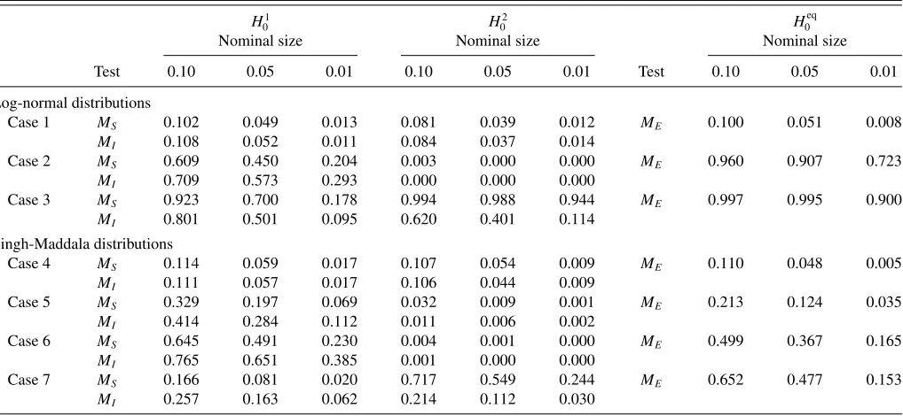
of the experiments, we used sample sizes ofN =M=500. The number of bootstrap replications was set to 500 to approximate thep-value in each Monte Carlo iteration, and 1000 iterations were performed for each experiment. The results for the Monte Carlo simulations are reported in Table 1. The table reports the proportion of times that the respective null hypothesis was rejected for three different nominal significance levelsα.
A number of features of the tests are worth nothing. The first series of experiments were based on the log-normal distribution, and in the first case the size properties of the tests were examined. Each of theMS,MI, andMEtest procedures led to the rejection
of the true null hypotheses at rates similar to the nominal size. There was a slight under rejection forH02; however, the under rejection was not severe, and the actual size of the tests were close to their nominal size. In terms of power, the test procedures appear to be quite similar where there is strong dominance. In Case 2, the tests detect the fact that the LC forX2 dominates that forX1. The hypothesesH01andH0eqare rejected with high probability. Note that the hypothesisH2
0 is rarely rejected in
this case—this feature of the test is related to the one-sided
Table 1. Monte Carlo rejection rates: independent sampling
H1
0 H
2
0 H
eq 0
Nominal size Nominal size Nominal size
Test 0.10 0.05 0.01 0.10 0.05 0.01 Test 0.10 0.05 0.01
Log-normal distributions
Case 1 MS 0.102 0.049 0.013 0.081 0.039 0.012 ME 0.100 0.051 0.008
MI 0.108 0.052 0.011 0.084 0.037 0.014
Case 2 MS 0.609 0.450 0.204 0.003 0.000 0.000 ME 0.960 0.907 0.723
MI 0.709 0.573 0.293 0.000 0.000 0.000
Case 3 MS 0.923 0.700 0.178 0.994 0.988 0.944 ME 0.997 0.995 0.900
MI 0.801 0.501 0.095 0.620 0.401 0.114
Singh-Maddala distributions
Case 4 MS 0.114 0.059 0.017 0.107 0.054 0.009 ME 0.110 0.048 0.005
MI 0.111 0.057 0.017 0.106 0.044 0.009
Case 5 MS 0.329 0.197 0.069 0.032 0.009 0.001 ME 0.213 0.124 0.035
MI 0.414 0.284 0.112 0.011 0.006 0.002
Case 6 MS 0.645 0.491 0.230 0.004 0.001 0.000 ME 0.499 0.367 0.165
MI 0.765 0.651 0.385 0.001 0.000 0.000
Case 7 MS 0.166 0.081 0.020 0.717 0.549 0.244 ME 0.652 0.477 0.153
MI 0.257 0.163 0.062 0.214 0.112 0.030
composite nature of the null hypothesis and is similar to the behavior of tests of one-sided restrictions on parameters. In Case 3, neither LC is dominant and the tests reject each null considered with very high probability, although the rejection is stronger for theMStest compared toMI.
The second series of experiments were based on the SM distribution. Case 4 provides a further comparison of the size properties of the tests. Again, the actual and nominal sizes of the tests were very similar. Although there was a slight overrejection ofH1
0, the discrepancy between actual and nominal sizes was
minor. It is useful to note that the sample sizes considered in the experiments were relatively small compared to many empirical applications and the fact that the actual sizes of the tests in these experiments are close to the nominal size is encouraging. In terms of power, the tests are able to detect the violation of
H01 andH0eqin Case 5, with the strong rejection of these nulls and, conversely, the rejection of true null ofH02is well below the nominal size. In Case 6, where the Lorenz dominance of
X2overX1 is stronger, the rejection rates forH1 0 andH
eq 0 are
greater, and the rejection of the true nullH2
0 is further below
the nominal size. In Case 7, with crossing LCs, theMS, MI,
andME tests detect the violation of the null hypotheses. The
null H1
0 is violated by a small amount over the bottom three
quintiles, which theMIis relatively better at detecting thanMS.
Conversely, the nullH2
0 is sharply violated over the top quintiles,
which theMS test is relatively superior at detecting. Even so,
both tests detect the violation of the false null sufficiently well to reject at rates well in excess of the nominal size.
4.2 Matched-Pair Sampling
The Monte Carlo experiments were repeated with the sim-ulated samples drawn from dependent distributions to reflect matched-pair sampling. Each case was repeated with identi-cal specifications for the marginal distributions and predeter-mined correlation. The method proposed by Cario and Nelson
(1997) for generating correlated random samples was adopted, which involved generating bivariate standard normal random variables (X1i,X˜2i) with correlation ˜ρ using the algorithm
˜
X2i =ρ.X˜ 1i+(1−ρ˜)2.X2i, where (X1i, X2i) are independent,
as in the initial series of experiments. For the log-normal sim-ulations, the variates (X1i,X˜2i) are demeaned and transformed
as in (4), and for the SM simulations the variates are demeaned, converted to uniform variates by applying the normal CDF, and then transformed to SM variates using the quantile function in (5). A numerical search over values of ˜ρwas performed to ob-tain the desired correlationρof the simulated log-normal and SM variates. The Monte Carlo experiments were performed for values of the correlation coefficientρ= {0.3,0.7,0.9}.These values are comparable to the correlation between family income and food expenditure, family income and nondurable expendi-tures, and pre-tax and post-tax income, respectively.
Results of the Monte Carlo simulation for the cases with
ρ=0.7 are reported inTable 2. Rejection rates for the simula-tions involving different values of correlation coefficients were very similar to those inTable 2and hence are not reported. As is evident fromTable 2, the tests under matched-pair sampling con-tinue to exhibit very good size characteristics. In terms of power performance, the tests tend to reject more strongly the false null hypotheses in Cases 2–3 and 5–7 under dependent sam-pling. Overall, series of small-scale Monte Carlo experiments indicate that each of the test procedures, under both indepen-dent and matched-pair sampling, exhibits good size and power properties. Further, when the sample size for the Monte Carlo experiments is increased slightly, the asymptotic properties are clearly reflected in enhanced size and power characteristics.
5. EMPIRICAL EXAMPLE
The methods for testing Lorenz dominance relations are il-lustrated with an analysis of the distribution of income and con-sumption in Australia. The data are from the Australia Bureau
Table 2. Monte Carlo rejection rates: matched-pair sampling (ρ=0.7)
H1
0 H02 H
eq 0
Nominal size Nominal size Nominal size
Test 0.10 0.05 0.01 0.10 0.05 0.01 Test 0.10 0.05 0.01
Log-normal distributions
Case 1 MS 0.088 0.047 0.013 0.097 0.054 0.014 ME 0.102 0.052 0.007
MI 0.090 0.052 0.014 0.104 0.064 0.013
Case 2 MS 0.697 0.555 0.259 0.002 0.001 0.000 ME 0.588 0.432 0.201
MI 0.832 0.735 0.468 0.001 0.001 0.001
Case 3 MS 0.956 0.765 0.193 0.995 0.985 0.939 ME 1.000 0.995 0.910
MI 0.871 0.593 0.128 0.662 0.429 0.131
Singh-Maddala distributions
Case 4 MS 0.096 0.042 0.007 0.116 0.060 0.015 ME 0.109 0.052 0.009
MI 0.100 0.047 0.010 0.123 0.069 0.019
Case 5 MS 0.425 0.270 0.092 0.021 0.005 0.000 ME 0.333 0.210 0.069
MI 0.608 0.464 0.203 0.007 0.003 0.000
Case 6 MS 0.861 0.748 0.438 0.003 0.000 0.000 ME 0.773 0.643 0.366
MI 0.966 0.923 0.752 0.000 0.000 0.000
Case 7 MS 0.249 0.137 0.039 0.865 0.722 0.363 ME 0.829 0.663 0.306
MI 0.371 0.240 0.088 0.297 0.137 0.042
of Statistics Household Expenditure Survey (HES) conducted in 1984, 1988/89, 1993/94, 1998/99, 2003/04, and 2009/10 (here-after referenced by the first year of the survey period). The income measure is gross annual family income. The consump-tion measure is expenditure on nondurables, consisting of food, alcohol, tobacco, fuel, clothing, personal care, medical care, transport, recreation, utilities, and current housing services. Cur-rent housing services for Cur-renters is equal to Cur-rent paid while for homeowners it is imputed from a regression of rent payments on a series of indicator variables for number of bedrooms and lo-cation of residence by survey year for the subsample of renters. The sample is restricted to families where the household refer-ence person is between 25 and 60 years of age.
Family income and consumption were divided by the adult equivalent scale (AES) equal to the square-root of family size. To minimize reporting errors, multiple-family households are excluded. The HES is a stratified random sample and for each observation there is an associated weight representing the in-verse probability of selection into the survey. The observational weights were multiplied by the number of family members to make the sample representative of individuals; the adjusted weights were used throughout the analysis.
Summary statistics are reported inTable 3. Nominal prices are inflated to 2010 real values using the CPI. The summary
statis-Table 3. HES 1984–2009 summary statistics
Income Consumption
Year Sample size Mean Std. Dev. Gini Mean Std. Dev. Gini
1984 2895 254.90 157.54 0.322 173.09 84.06 0.251 1988 4654 263.26 180.79 0.323 173.02 84.04 0.247 1993 5396 265.49 197.15 0.346 186.50 94.08 0.247 1998 4645 296.11 198.85 0.342 201.40 96.89 0.248 2003 4583 325.97 227.25 0.330 215.14 104.75 0.249 2009 5009 408.75 364.59 0.361 251.42 131.73 0.260
tics show that the mean budget share of the nondurable commod-ity bundle was 68% in 1984. Over the sample period, nondurable consumption grew at an average annual rate of 2.36% while in-come grew at an average annual rate of 2.53%. Point estimates for the Gini coefficient suggest a substantial increase in income inequality, and a minor change in consumption inequality, over the 25-year period.
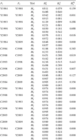
The first comparisons examine changes in the distribution of individual equivalent income over time.Table 4 presents the
p-values for the tests of the null hypothesis that Distribution 1 weakly Lorenz dominated Distribution 2, against the alternative that the null is false. To calculate thep-values, 2000 bootstrap repetitions were used to simulate the distribution of the test statistics. The first two rows of the table are for the test with Distribution 1 corresponding to 1984 income and Distribution 2 corresponding to 1988 income. The results show that neither null of dominance,H084orH088, can be rejected at the 5% level of sig-nificance. Thep-value for the null of LC equality of 0.159, which is similar to the bound based on the Bonferroni inequality for
MSof 0.146, does not lead to rejection at conventional levels of
significance. The tests indicate that the two income distributions were “equally unequal.” The following two rows show the null hypothesis that the 1988 income distribution Lorenz dominated the 1993 distribution cannot be rejected, while the converse null, that the 1993 distribution dominated 1988, can be rejected at the 5% level of significance. Strong Lorenz dominance of the 1988 income distribution over the 1993 distribution can be inferred at conventional levels of significance. Comparison of the 1993 and 1998 income distributions shows that the two LCs are equal, while the 2003 distribution is found to strongly Lorenz dominate both the 1998 and 2009 distributions at the 10% level of sig-nificance. Across the full observation period, the 1984 income distribution strongly Lorenz dominates the 2009 income distri-bution. The increase in income inequality over the 1984–2009 period was concentrated in the 1988–93 and 2003–09 subperi-ods, where the former coincided with the severe recession of
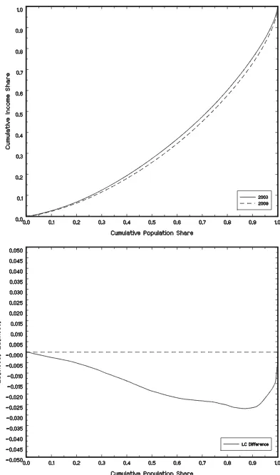
Figure 1. Comparison of Australian gross income Lorenz curves based on samples from the ABS Household Expenditure Survey for 2003 and 2009: (a) Gross income Lorenz curves for 2003 (——) and 2009 (- - - -); (b) Difference in gross income Lorenz curves 2009–2003 (——) and equality (- - - -).
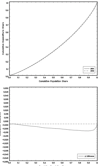
Figure 2. Comparison of Australian nondurable expenditure Lorenz curves based on samples from the ABS Household Expenditure Survey for 2003 and 2009: (a) Nondurable expenditure Lorenz curves for 2003 (——) and 2009 (- - - -); (b) Difference in nondurable expenditure Lorenz curves 2009–2003 (——) and equality (- - - -).
Table 4. P-values for Lorenz Dominance Tests
Y1984 Y1988 MS 0.611 0.079 0.159
MI 0.486 0.640
Y1988 Y1993 MS 0.942 0.002 0.001
MI 0.913 0.001
Y1993 Y1998 MS 0.129 0.699 0.266
MI 0.221 0.601
Y1998 Y2003 MS 0.030 0.181 0.066
MI 0.030 0.542
Y2003 Y2009 MS 0.976 0.011 0.016
MI 0.972 0.001
Y1984 Y2009 MS 0.846 0.000 0.000
MI 0.857 0.000
C1984 C1988 MS 0.188 0.550 0.385
MI 0.233 0.630
C1988 C1993 MS 0.451 0.306 0.619
MI 0.442 0.405
C1993 C1998 MS 0.216 0.515 0.443
MI 0.498 0.399
C1998 C2003 MS 0.431 0.415 0.807
MI 0.463 0.368
C2003 C2009 MS 0.886 0.063 0.127
MI 0.907 0.050
C1984 C2009 MS 0.965 0.193 0.358
MI 0.969 0.093
C1984 Y1984 MS 0.974 0.000 0.000
MI 0.974 0.000
C1988 Y1988 MS 0.991 0.000 0.000
MI 0.991 0.000
C1993 Y1993 MS 0.974 0.000 0.000
MI 0.974 0.000
C1998 Y1998 MS 0.995 0.000 0.000
MI 0.995 0.000
C2003 Y2003 MS 0.949 0.000 0.000
MI 0.974 0.000
C2009 Y2009 MS 0.989 0.000 0.000
MI 0.989 0.000
Y1984 C2009 MS 0.000 0.686 0.000
MI 0.000 0.824
C1984 Y2009 MS 0.991 0.000 0.000
MI 0.991 0.000
1990/1991 while the latter includes the global financial crisis that began in 2007.
Consumers with access to credit facilities may smooth tran-sitory fluctuates in current income. It is therefore of interest to examine changes in consumption inequality over time. In com-paring across surveys, relative inequality in the distribution of consumption shows much greater stability. The consumption LCs between adjacent surveys in the 1984–2003 period were found to coincide. The 2003 consumption distribution weakly Lorenz dominated the 2009 distribution, although the null of LC equality is not rejected at conventional levels of significance (the Bonferroni bound on thep-value from the sequential application ofMSis 0.126). The income and consumption LCs for the 2003
and 2009 samples are plotted in Figures1and2, respectively, showing the greater increase in income inequality between the two survey years. The findings suggest that the increases in in-come inequality coinciding with the 1990/1991 recession and
the onset of the global financial crisis in 2007 had a transitory component that households were largely able to smooth.
The lower panels ofTable 4present several additional com-parisons. The standard life-cycle model of consumption implies that the distribution of nondurable consumption will be more equal than the distribution of current income at a point in time. This hypothesis was tested with the bootstrap procedure adapted for matched pair sampling to replicate the dependence in the data. The comparison of the empirical income and consumption distributions for each survey year strongly supports this hypoth-esis. Further, comparing income and consumption at different points in time, the consumption distribution in 2009 strongly Lorenz dominated the distribution of income in 1984 (the most equal income distribution). Less surprising, the 1984 consump-tion distribuconsump-tion strongly Lorenz dominated the 2009 income distribution.
Overall, the Lorenz dominance tests show a rise in income inequality in Australia between 1984 and 2009, though con-sumption inequality remained stable. The empirical results sug-gest that households were generally insured against shocks to the income process over the observation period. The test results show that the distribution of consumption was more equal than the distribution of income at each point in time, and over the study period. In terms of the performance of the two tests of Lorenz dominance, both gave essentially the same result, which suggests that either may be used in practice.
6. CONCLUSION
In this article we proposed two methods for testing for Lorenz dominance, along with a test of LC equality, based on samples from two, potentially dependent, populations. The tests pre-sented are fully nonparametric and consistent, being based on global comparisons of the empirical LCs. Although the pro-posed test statistics have nonstandard and case-specific limiting distributions, we were able to show that asymptotically valid inferences could be drawn using the bootstrap. Each of the tests were shown to have a good performance in quite small sam-ples and were illustrated in the context of an empirical example comparing income and consumption LCs for Australia over the period 1984–2009/10.
APPENDIX: PROOFS OF RESULTS
Proof of Lemma 1: Suppose thatH1
0 holds thenφ≤0,
F(φ)≤F(φ−φ)=F(0)=0.
On the other hand, F(φ)≤0 implies thatφ≤0 by Property 1(ii). Clearly, underH11 we haveF(φ)>0 by Property 1(ii). The converse follows easily since ifF(φ)>0 then it cannot be the case thatH01is true since if it were true, that is,φ≤0, then using Property 1(i),
0<F(φ)≤F(φ−φ)=F(0)=0,
which is false. Consequently,H11must be true.
Proof of Lemma 2: For Property 1(i), we have
φ∗(p)≤φ∗(p)−φ′(p)∀p
so that S is easily seen to satisfy the property whileI does by properties of the integral, and sinceφ∗(p)>0=⇒φ∗(p)−
φ′(p)>0, hence
φ∗(p)1(φ∗(p)>0)≤(φ∗(p)−φ′(p))1(φ∗(p)−φ′(p)>0).
For Property 1(ii), we have that if there is apsuch thatφ∗(p)>0 then
S(φ∗)≥φ∗(p)>0
while continuity ofφ∗ implies that there is a neighborhood of
pon whichφ∗(p′)> ε >0 for allp′such that|p′−p|< δ, so that
I(φ∗)≥
p+δ p−δ
φ∗(p′)1(φ∗(p′)>0)dp
>
p+δ p−δ
εdp=2δε >0.
For Property 1(iii), forSwe have
S(φ∗)≤S(φ′+φ∗−φ′)≤S(φ′)+S(φ∗−φ′)
so,
S(φ∗)−S(φ′)≤S(φ∗−φ′)≤ φ∗−φ′;
reversingφ′andφ∗we have,
S(φ′)−S(φ∗)≤ φ∗−φ′
so,
−φ∗−φ′ ≤S(φ∗)−S(φ′)
and Property 1(iii) follows. ForI, we have that
|φ∗(p)1(φ∗(p)>0)dp−φ′(p)1(φ′(p)>0)| ≤ |φ∗(p)−φ′(p)|,
which is obvious whenφ∗(p)>0 andφ′(p)>0 and also when both are negative. When,φ∗(p)>0 andφ′(p)≤0, we have
|φ∗(p)1(φ∗(p)>0)dp−φ′(p)1(φ′(p)>0)| = |φ∗(p)|
≤ |φ∗(p)−φ′(p)|
and similarly for the other case. Hence,
|I(φ∗)−I(φ′)| ≤
1
0
|φ∗(p)−φ′(p)|dp≤ φ∗−φ′.
Property 1(iv) is obvious forSand follows forIby linearity of the integral operator and the fact that
cφ∗(p)>0⇐⇒φ∗(p)>0.
For Property 1(v), letφ′ andφ∗ be continuous functions and letβ ∈(0,1). Then forS, the result follows by properties of supremum since
S(βφ′+(1−β)φ∗)≤S(βφ′)+S((1−β)φ∗)
=βS(φ′)+(1−β)S(φ∗).
For the functionalI, we have that
I(βφ′+(1−β)φ∗)
=
1
0
βφ′(p)1(βφ′(p)+(1−β)φ∗(p)>0)dp
+
1
0
(1−β)φ′(p)1(βφ′(p)+(1−β)φ∗(p)>0)dp
≤β
1
0
φ′(p)1(βφ′(p)>0)
+
1 0
(1−β)φ′(p)1((1−β)φ∗(p)>0)
=βI(φ′)+(1−β)I(φ∗)
using the following facts,
βφ′(p)1(βφ′(p)+(1−β)φ∗(p)>0)≤βφ′(p)1(βφ′(p)>0)
(1−β)φ′(p)1(βφ′(p)+(1−β)φ∗(p)>0)
≤(1−β)φ′(p)1((1−β)φ∗(p)>0).
To see that these hold, consider the first expression. There are two possible ways in which βφ′(p)+(1−β)φ∗(p)>0 holds. First, it could be thatβφ′(p)>0,in which case the expression on the left is equal to the expression on the right. Second, it could be thatβφ′(p)<0,in which case the left hand side is negative while the right-hand side is positive. Thus, the inequal-ity holds, and the same argument can be applied to the second
expression.
Proof of Lemma 4: (i) Under the null hypothesis, φ(p)=
L2(p)−L1(p)≤0 for allp∈(0,1).By Property 1(i) and (iv),
we then have that
TnF( ˆφ) ≤ TnF( ˆφ−φ)=F(Tn( ˆφ−φ))
=⇒F( ¯L)
with the weak convergence following from Lemma 3(ii) and the continuous mapping theorem that applies by Property 1(iii). Note that the 1−αquantile is positive by the fact thatF( ¯L)≤0 is equivalent to sup ¯L(p)≤0 using Property 1(ii) and,
P(sup ¯L(p)≤0)<1/2
using the fact that ¯L is a separable mean zero Gaussian pro-cess. The quantile is finite for any 1/2> α >0 using Borell’s inequality (stated as proposition A.2.1 by van der Vaart and Wellner1996). Finally, uniqueness of the quantile follows from the fact thatF is convex using proposition 11.1 by Davydov, Lifshits, and Smorodina (1998).
For (ii) by Lemma 3(i) and using Property 1(i) and (iii),
F( ˆφ)→p F(φ)>0 so thatTnF( ˆφ)
p
→ ∞.
Proof of Proposition 1: The LC is a Hadamard differentiable functional of the empirical distribution function following the results by Bhattacharya (2005). We must establish that the boot-strap applied to the empirical distributions yields processes with covariance properties corresponding to those for the empirical distributions ofX1 andX2under Assumption 2(IS) or 2(MP).
In the case of Assumption 2(IS), bootstrap empirical processes are, respectively (see van der Vaart and Wellner1996, 3.6),
G1n(x1)=
whereM1iandM2iare multinomial random variables (with
pa-rametersn1,n2 and probabilities 1/n1 and 1/n2, respectively)
independent of the sample and also independent of each other. It is easy to verify that, conditional on the sample, these are inde-pendent mean zero processes with covariance kernels given by,
E(Gj n(xj0)Gj n(xj0)|Xj)=Fˆj(xj0)−Fˆj(xj0) ˆFj(xj1) (6)
forxj0≤xj1 and that this converges to the covariance kernel
of the limiting process corresponding to the empirical process based on the empirical distribution.
On the other hand under Assumption 2(MP), we have boot-strap empirical processes
using the same multinomial variable Mi (with parameter n
and probabilities 1/n). In this case, the covariance kernel of each process has the same form as (6) but the processes are correlated since
E(G1n(x1)G2n(x2)|X)=Fˆ(x1, x2)−Fˆ1(x1) ˆF2(x2).
Thus, the bootstrap processes, in the limit, have a correlation structure corresponding to (2).
The result then follows using the delta method for the boot-strap (van der Vaart and Wellner1996, 3.9.11) and the continu-ous mapping theorem. In particular, note that the decision rule is equivalent to the rule thatTnF( ˆφ)>cˆn(α) with,
ˆ
cn(α)=inf{t :P(TnF( ˆφ∗(p)−φˆ(p))> t|X)≤α),
where we condition on the sample(s) in computing the probabil-ity. With the Hadamard differentiability of the LC and Property 1(iii) and (iv) of the mapF, we have that
TnF( ˆφ∗(p)−φˆ(p))→F( ¯L)
in probability givenXso that
ˆ
cn(α) p
−→c(α)=inf{t :P(F( ¯L)> t)≤α)},
where the latter is strictly positive, finite, and unique given Lemma 4. The result then follows using Lemma 4.
ACKNOWLEDGMENTS
The authors thank Keisuke Hirano, the associate editor, and two referees for useful suggestions. The research was partially supported by the Australian Research Council and NSF grant SES-0196372. STATA and GAUSS programs for implement-ing the tests in this article are available on request from the authors.
[Received December 2011. Revised April 2013.]
REFERENCES
Andrews, D. W. K. (1997), “A Conditional Kolmogorov Test,”Econometrica, 65, 1097–1128. [2]
Atkinson, A. B. (1970), “On the Measurement of Inequality,”Journal of Eco-nomic Theory, 2, 244–263. [1,2]
——— (1987), “On the Measurement of Poverty,”Econometrica, 55, 749–764. [2]
Barrett, G. F., and Donald, S. G. (2003), “Consistent Tests for Stochastic Dom-inance,”Econometrica, 71, 71–104. [2]
Beach, C. M., and Davidson, R. (1983), “Distribution-Free Statistical Inference With Lorenz Curves and Income Shares,”Review of Economic Studies, 50, 723–735. [1,4]
Bhattacharya, D. (2005), “Asymptotic Inference From Multi-Stage Samples,” Journal of Econometrics, 126, 145–171. [2,3,12]
——— (2007), “Inferences on Inequality From Household Surveys,”Journal of Econometrics, 137, 674–707. [1,4]
Bishop, J. A., Formby, J. P., and Smith, W. J. (1991a), “Lorenz Dominance and Welfare: Changes in the U.S. Distribution of Income, 1967–1986,”Review of Economics and Statistics, 73, 134–139. [1]
——— (1991b), “International Comparisons of Income Inequality: Tests for Lorenz Dominance Across Nine Countries,” Economica, 58, 461–477. [1]
Cario, M. C., and Nelson, B. L. (1997), “Modeling and Generating Random Vectors With Arbitrary Marginal Distributions and Correlation Matrix,” Technical Report 50, Department of Industrial Engineering and Management Sciences, Northwestern University, Evanston, IL. [7]
Dardanoni, V., and Forcina, A. (1999), “Inference for Lorenz Curve Orderings,” Econometrics Journal, 2, 49–75. [1]
Davidson, R., and Duclos, J.-Y. (2000), “Statistical Inference for Stochastic Dominance and for the Measurement of Poverty and Inequality,” Economet-rica, 68, 1435–1464. [1]
Davies, J. B., Green, D. A., and Paarsch, H. J. (1998), “Economic Statistics and Social Welfare Comparisons: A Review,” inHandbook of Applied Economic Statistics, eds. A. Ullah and D.E.A. Giles, New York: CRC Press, chap. 1. [1]
Davydov, Y. A., Lifshits, M. A., and Smorodina, N. V. (1998),Local Proper-ties of Distributions of Stochastic Functionals, Providence, RI: American Mathematical Society. [3,12]
Deaton, A. S. (1997),The Analysis of Household Surveys: Microeconometric Analysis for Development Policy, Baltimore, MD: Johns Hopkins University Press for The World Bank. [2]
Goldie, C. M. (1977), “Convergence Theorems for Empirical Lorenz Curves and Their Inverses,” Advances in Applied Probability, 9, 765–791. [4]
Lambert, P. J. (1993), The Distribution and Redistribution of Income: A Mathematical Analysis (2nd ed.), Manchester: Manchester University Press. [2]
Linton, O., Maasoumi, E., and Whang, Y. J. (2005), “Consistent Testing for Stochastic Dominance: A Subsampling Approach,”Review of Economic Studies, 72, 735–765. [2]
McFadden, D. (1989), “Testing for Stochastic Dominance,” inStudies in the Economics of Uncertainty: In Honor of Josef Hadar, eds. T.-B. Fomby and T.-K. Seo, New York: Springer, pp. 113–134. [2]
Van der Vaart, A. W., and Wellner, J. A. (1996),Weak Convergence and Empir-ical Processes: With Applications to Statistics, New York: Springer-Verlag. [4,12,13]
Wilfling, B., and Kramer, W. (1993), “The Lorenz-Ordering of Singh-Maddala Income Distributions,”Economics Letters, 43, 53–57. [6]
Wolak, F. A. (1989), “Testing Inequality Constraints in Linear Econometric Models,”Journal of Econometrics, 41, 205–235. [1]