Full Terms & Conditions of access and use can be found at
http://www.tandfonline.com/action/journalInformation?journalCode=ubes20
Download by: [Universitas Maritim Raja Ali Haji] Date: 12 January 2016, At: 17:32
Journal of Business & Economic Statistics
ISSN: 0735-0015 (Print) 1537-2707 (Online) Journal homepage: http://www.tandfonline.com/loi/ubes20
Forecast Combination With Entry and Exit of
Experts
Carlos Capistrán & Allan Timmermann
To cite this article: Carlos Capistrán & Allan Timmermann (2009) Forecast Combination With Entry and Exit of Experts, Journal of Business & Economic Statistics, 27:4, 428-440, DOI: 10.1198/jbes.2009.07211
To link to this article: http://dx.doi.org/10.1198/jbes.2009.07211
Published online: 01 Jan 2012.
Submit your article to this journal
Article views: 173
View related articles
Forecast Combination With Entry
and Exit of Experts
Carlos C
APISTRÁNBanco de México, Dirección General de Investigación Económica, Av. 5 de Mayo No. 18, 4o. Piso, Col. Centro, 06059, México DF, México (ccapistran@banxico.org.mx)
Allan T
IMMERMANNRady School of Management and Department of Economics, University of California, San Diego, 9500 Gilman Drive, La Jolla, CA 92093-0553, and CREATES, University of Aarhus (atimmerm@ucsd.edu)
Combination of forecasts from survey data is complicated by the frequent entry and exit of individual forecasters which renders conventional least squares regression approaches infeasible. We explore the consequences of this issue for existing combination methods and propose new methods for bias-adjusting the equal-weighted forecast or applying combinations on an extended panel constructed by back-filling missing observations using an EM algorithm. Through simulations and an application to a range of macro-economic variables we show that the entry and exit of forecasters can have a large effect on the real-time performance of conventional combination methods. The bias-adjusted combination method is found to work well in practice.
KEY WORDS: Bias-adjustment; EM algorithm; Real-time Data; Survey of Professional Forecasters.
1. INTRODUCTION
Survey forecasts provide an ideal data source for investigat-ing real-time forecastinvestigat-ing performance. By construction, such forecasts were computed in real time and so do not suffer from the potential look-ahead biases associated with forecasts con-structed ex post from an econometric model due to the effects of parameter estimation, model selection (Pesaran and Tim-mermann2005), or data revisions (Amato and Swanson2001; Croushore and Stark2001).
Surveys include multiple participants and so a natural ques-tion becomes how best to select or combine individual fore-casts. Moreover, a largely ignored issue is that most surveys take the form of unbalanced panels due to the frequent entry, exit, and reentry of individual forecasters. This is a general problem and affects, inter alia, the Livingston survey, the Sur-vey of Professional Forecasters, Blue Chip forecasts, the surSur-vey of the Confederation of British Industry, Consensus Forecasts, and surveys of financial analysts’ forecasts.
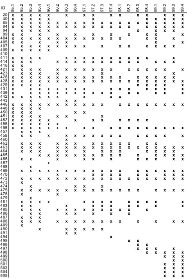
As an illustration of this problem, Figure1shows how partic-ipation in the Survey of Professional Forecasters evolved over the 5-year period from 1995 to 1999. Each quarter, participants are asked to predict the implicit price deflator for the Gross Do-mestic Product. Forecasters constantly enter, exit, and reenter following a period of absence, creating problems for standard combination approaches that rely on estimating the covariance matrix for the individual forecasts. Such approaches are not fea-sible with this type of data since many forecasters may not have overlapping data and so the covariance matrix cannot be esti-mated.
This paper considers ways to recursively select or combine survey forecasts in the presence of such missing observations. We consider both conventional methods and some new ap-proaches. The first category includes the previous best forecast, the equal-weighted average, odds ratio methods in addition to least squares, and shrinkage methods modified by trimming
forecasts from participants who do not report a minimum num-ber of data points. The second category includes a method that projects the realized value on a constant and the equal-weighted forecast. This projection performs a bias correction in response to the strong evidence of biases in macroeconomic survey fore-casts (Zarnowitz1985; Davies and Lahiri1995) and among fi-nancial analysts (Hong and Kubik2003). Although this method is parsimonious and only requires estimating an intercept and a slope parameter, we also consider using the SIC to choose between the simple and bias-adjusted average forecast. Finally, we use the EM algorithm to fill out past missing observations when forecasters leave and rejoin the survey and combine the forecasts from the extended panel.
We compare the (“pseudo”) real-time forecasting perfor-mance of these methods through Monte Carlo simulations in the context of a common factor model that allows for bias in the individual forecasts, dynamics in the common factors, and het-erogeneity in individual forecasters’ ability. In situations with a balanced panel of forecasts, the least squares combination methods perform quite well unless the cross-section of fore-casts (N) is large relative to the length of the time series (T). If the parameters in the Monte Carlo simulations are chosen so that equal weights are sufficiently suboptimal in popula-tion, least-squares combination methods dominate the equal-weighted forecast. Interestingly, the simple bias-adjusted mean outperforms regression-based and shrinkage combination fore-casts in most experiments.
In the simulations that use an unbalanced panel of fore-casts calibrated to match actual survey data, the simulated
© 2009American Statistical Association Journal of Business & Economic Statistics October 2009, Vol. 27, No. 4
DOI:10.1198/jbes.2009.07211
428
Figure 1. Participants in the survey of professional forecasters (PGDP).Notes:The ID corresponds to the identification number assigned to each forecaster in the survey. The columns represent the quarter when the survey was taken. Thexs show when a particular forecaster responded to the PGDP part of the survey and provided a one-step-ahead forecast for inflation.
real-time forecasting performance of the least squares com-bination methods deteriorates relative to that of the equal-weighted combination. This happens because the panel of casters must be trimmed to get a balanced subset of fore-casts from which the combination weights can be estimated by least squares methods. This step entails a loss of information relative to using the equal-weighted forecast which is based on the complete set of individual forecasts. The bias-adjusted
mean forecast continues to perform well in the unbalanced panel.
We finally evaluate the selection and combination methods using survey data on 14 time series covering a range of macro-economic variables. Consistent with other studies (e.g., Stock and Watson2001,2004), we find that most methods are domi-nated by the simple equal-weighted average. However, there is evidence for around half of the variables that the bias-adjusted
combination method—particularly when refined by the selec-tion step based on the SIC—improves upon the equal-weighted average. We show that this is related to evidence of biases in the equal-weighted average.
The plan of the paper is as follows. Section2describes meth-ods for estimating combination weights. Section3conducts the Monte Carlo simulation experiment while Section 4provides the empirical application. Section5concludes.
2. SELECTION AND COMBINATION METHODS
This section introduces the methods for selecting individ-ual forecasts or combining multiple forecasts that will be used in the simulations and empirical application. We let Yˆti+h|t be the ith survey participant’s period-t forecast of the outcome variable Yt+h, where h is the forecast horizon, i=1, . . . ,Nt andNt is the number of forecasts reported at timet. Individ-ual forecast errors are then given by eit+h|t =Yt+h− ˆYti+h|t, while the vector of forecast errors is et+h|t=ιYt+h− ˆYt+h|t, whereYˆt+h|t =(Yˆt1+h|t, . . . ,YˆtN+h|t)′ andι is an Nt×1 vector of ones. Suppose that Yt+h∼(µy, σy2),Yˆt+h|t∼(μ,yˆyˆ)and Cov(Yt+h,Yˆt+h|t)=σyyˆ, where for simplicity we omit time and horizon subscripts on the moments. Forecast combination methods entail finding a vector of weights,ω, that minimize the mean squared error (MSE):
E
e′t+h|tet+h|t=(µy−ω′μ)2+σy2+ω′yˆyˆω−2ω′σyyˆ. (1) Selection and combination methods differ in how they esti-mate the moments in (1) and which restrictions they impose on the weights.
Previous Best Forecast
Rather than obtainingωthrough estimation, one can simply pick the best forecast based on past forecasting performance, that is,Yˆt∗+h|t= ˆYi
This corresponds to setting a single element ofωequal to one and the remaining elements to zero. Note that the ranking of the various forecasts follows a stochastic process that may lead to shifts in the selected forecast as new data emerges.
Equal-Weighted Average
By far the most common combination approach is to use the equal-weighted forecast
which is simple to compute even for unbalanced panels of forecasts and has proven surprisingly difficult to outperform (Clemen 1989; Stock and Watson 2001, 2004; Timmermann 2006). Intuition for why this approach works well is that, in the presence of a common factor in the forecasts, the first principal component can be approximated by the 1/N combination. In
population, the equal-weighted average is optimal in the sense that it minimizes (1) when the forecast error variances are the same and forecast errors have identical pairwise correlations, that is, in the absence of heterogeneity among individual fore-casters, but it will generally be suboptimal under heterogeneity. Importantly, optimality of the 1/Nweights also requires that the forecasts be unbiased (μ=µyι)and the additional constraint
ω′ι=1.
Least Squares Estimates of Combination Weights
A simple way to obtain estimates of the combination weights is to perform a least squares regression of the outcome vari-able,Yt, on a constant,ω0, and the vector of forecasts,Yˆt|t−h=
(Yˆt1|t−h, . . . ,YˆtN|t−h)′.Population optimal values of the intercept and slope parameters in this regression are:
ω∗0=µy−ω∗′μ,
(4)
ω∗=−1yˆyˆσyˆy.
Granger and Ramanathan (1984) consider three versions of the least squares regression:
(i) Yt=ω0+ω′Yˆt|t−h+εt,
(ii) Yt=ω′Yˆt|t−h+εt, (5)
(iii) Yt=ω′Yˆt|t−h+εt, s.t.ω′ι=1.
The first and second of these regressions can be estimated by standard OLS, the only difference being that the second equa-tion omits an intercept term. The third regression omits an in-tercept and can be estimated through constrained least squares. The first regression does not require the individual forecasts to be unbiased since any bias is absorbed through the intercept,
ω0. In contrast, the third regression is motivated by an assump-tion of unbiasedness of the individual forecasts. Imposing that the weights sum to one then guarantees that the combined fore-cast is also unbiased.
The main advantage of this approach is that it applies under general correlation patterns, including in the presence of strong heterogeneity among forecasters. On the other hand, estimation error is known to be a major problem whenN is large orT is small. Another problem is that the approach is poor at handling unbalanced datasets for which the full covariance matrix cannot be estimated. In such cases, minimum data requirements must be imposed and the set of forecasts trimmed. For example, one can require that forecasts from a certain minimum number of (not necessarily contiguous) common periods be available.
Inverse MSE
To reduce the effect of parameter estimation errors, we apply a weighting scheme which, for forecasters with a sufficiently long track record, uses weights that are inversely proportional to their historical MSE values, while using equal-weights for the remaining forecasters (normalized so the weights sum to one).
Shrinkage
Stock and Watson (2004) propose shrinkage towards the arithmetic average of forecasts. Letωˆitbe the least-squares esti-mator of the weight on theith model in the forecast combination obtained, for example, from one of the regressions in (5). The combination weights considered by Stock and Watson take the form
ωit=ψtωˆit+(1−ψt)(1/Nt),
(6)
ψt=max(0,1−κNt/(T−1−Nt−1)).
Larger values ofκ imply a lowerψtand thus a greater degree of shrinkage towards equal weights. As the sample size,T, rises relative to the number of forecasts,Nt, the least squares estimate gets a larger weight, thus putting more weight on the data in large samples.
Odds Matrix Approach
The odds matrix approach (Gupta and Wilton 1988) com-putes the combination of forecasts as a weighted average of the individual forecasts where the weights are derived from a ma-trix of pair-wise odds ratios. The odds mama-trix,O, contains the pair-wise probabilitiesπijthat theith forecast will outperform thejth forecast in the next realization, that is,oij=ππij
ji. We
esti-mateπij fromπij= aij
(aij+aji), whereaij is the number of times
forecast i had a smaller absolute error than forecast j in the historical sample. The weight vector,ω, is obtained from the solution to(O−NtI)ω=0,whereIis the identity matrix. We follow Gupta and Wilton and use the normalized eigenvector associated with the largest eigenvalue ofO.
Bias-Adjusted Mean
As noted in theIntroduction, there is strong empirical evi-dence that individual survey participants’ forecasts are biased. Moreover, equal-weighted averages of biased forecasts will themselves in general be biased. To deal with this, we propose a simple bias adjustment of the equal-weighted forecast,Y¯t+h|t:
˜
Yt+h|t=α+βY¯t+h|t. (7) To intuitively motivate the slope coefficient in (7),β, notice that there always exists a scaling factor such that, at a given point in time, the product of this and the average forecast is unbiased. To ensure that on average (or unconditionally) the combined forecast is unbiased, we further include a constant in (7).
This extension of the equal-weighted combination uses the full set of individual forecasts (incorporated in the equal-weighted average) and only requires estimating two parameters,
αandβ, which can be done through least squares regression. The method is therefore highly parsimonious and so is less af-fected by estimation error than regression-based methods such as (5), particularly when N is large. For balanced panels the method can be viewed as a special case of the general Granger– Ramanathan regression (5), part (i), although this does not hold with missing observations.
To see more rigorously when the bias-adjustment method is optimal, notice that under homogeneity in the covariance structure of(Yt+h,Yˆt+h|t), we can write (by theorem 8.3.4 in
Graybill 1983) −1yˆyˆ =c1IN+c2ιι′, σyyˆ =c3ι, where ci are constant scalars and IN is theN×N identity matrix, so that from (4),ω∗=c3(c1+Nc2)ι, whileω0∗=µy−ω∗′μ. Setting
β=c3N(c1+Nc2)andα=µy−c3(c1+Nc2)ι′μ, we see that the optimal combination takes the form in (7).
The bias-adjustment method will thus be optimal if the only source of heterogeneity is individual-specific biases, although it will not be (asymptotically) optimal in the presence of het-erogeneity in the variance or covariance of the forecast errors. The reason is that the intercept term,α, corrects for arbitrary forms of biases, independent of their heterogeneity. This is em-pirically important; for example, Elliott, Komunjer, and Tim-mermann (2008) find evidence of considerable heterogeneity in individual-specific biases.
To see when a slope coefficient,β, different from one may occur, suppose that both the outcome and the forecasts are driven by a single common factor, F, but that, due to mis-specification, the individual forecasts contain an extraneous source of uncorrelated noise,εi:Y=F+εY,Yˆi=F+εi, where Var(F)=σF2, Var(εi)=σε2, Cov(εi, εj)=0 for all i=j, and Cov(εi, εy)=0. Then one can show thatω∗=ισF2/(σε2+NσF2). The optimal weights are thus only equal to(1/N)ιin the spe-cial case whereσε2=0, that is, if there is no misspecification in the individual forecasts. By including a slope coefficient,
β=NσF2/(σε2+NσF2), Equation (7) can handle this type of (ho-mogenous) misspecification.
Model Selection Approach (SIC)
Following Swanson and Zeng (2001), this approach uses the Schwarz Information Criterion (SIC: Schwarz1978) to select among the simple and bias-adjusted equal-weighted average. The bias-adjusted forecast requires estimating two additional parameters and so only gets selected provided that its fit im-proves sufficiently on the equal-weighted forecast.
EM Algorithm
Suppose that the individual forecasts follow a local level model
ˆ
Yti+h|t=xit+ξti, ξti∼N(0, σξ2i),
(8)
xit+1=xit+ηit, ηti∼N(0, ση2i),
whereξtiandηtiare mutually independent, cross-sectionally in-dependent as well as inin-dependent ofx1.We use the Expectation Maximization (EM) algorithm (Watson and Engle1983; Koop-man 1993) to recursively estimate the two variancesσ2
ξi and
σ2
ηi. This approach uses the smoothed state to back-fill missing
forecasts whenever a survey participant has left the survey but rejoins at a later stage. The least squares combination approach in (5), part (i), is then used on the reconstructed panel of fore-casts.
It is difficult to obtain analytical results for the forecasting performance of the above methods. The forecasts are likely to reflect past values of the predicted series and so cannot be con-sidered strictly exogenous, making it very hard to character-ize the finite sample distribution of the mean squared forecast errors. The unbalanced panel structure of the surveys further complicates attempts at analytical results. For this reason we next turn to simulations and empirical applications to study the performance of the selection and combination approaches.
3. MONTE CARLO SIMULATIONS
To analyze the determinants of the performance of the var-ious forecast combination methods, we conduct a series of Monte Carlo experiments in the context of a simple two-factor model: with diagonal autoregressive matrix BF and uncorrelated in-novations,εFt+1∼N(0, σ
2
εF). This model is simply a different
representation of a setup where at time t forecasters receive noisy signals that are imperfectly correlated with the future fac-tor realizations,F1t+1andF2t+1.
We let the sample size,T, vary from 50 to 100 and 200 and let the number of forecasts (N) assume values of 4, 10, and 20. This covers situations with largeN relative to the sample size
T (e.g., N=20,T =50) as well as situations with plenty of data points relative to the number of estimated parameters (e.g.,
N=4,T =200). All forecasts are one step ahead, simulated out of sample, and are computed based on recursive parameter estimates using only information available at the time of the forecast.
The first experiments assume that the individual forecasts are unbiased and setµy=µi=0(i=1, . . . ,N). In all experiments but number 4 we assume thatβi1=βi2=0.5 (i=1, . . . ,N). In experiment 1 all parameters (except forBFwhich equals zero) are set equal to one, and we solve for σε2
i (identical for alli)
so the optimal weights are identical and sum to unity. In ex-periments 2–7 we set σε2
i so that the regression coefficient of
Yt+1on the individual forecastsYˆti+1|t is unity. Factor dynam-ics is introduced in experiment 3 by lettingBF=0.9×I. Het-erogeneity in the individual forecasters’ ability is introduced in two ways: first, by drawing the factor loadings,βif, from a Beta(1,1)distribution centered on 0.5 (experiment 4) and, sec-ond, by drawing the inverse of the variance of the idiosyncratic errors,σε−2i , from a Gamma(5,5)distribution (experiment 5). To allow for the possibility that different forecasts capture dif-ferent predictable components (thus enhancing the role of fore-cast combinations over the individual models), experiment 6 considers a scenario where different groups of forecasts load on different factors. Finally, forecast biases are introduced in experiment 7 by allowing for a nonzero intercept. Additional details are provided in Table1.
3.1 Balanced Panel of Forecasters
The first set of results assumes a balanced panel of forecasts. Panel A of Table1reports simulated out-of-sample MSE values computed relative to the MSE value associated with the equal-weighted forecast (which is thus always equal to unity).
In the first experiment, the simple equal-weighted forecast performs best—imposing a true constraint ensures efficiency gains. For the same reason, the combination that excludes an intercept and constrains the weights to sum to unity is best among the regression-based methods. The improvement over the most general least squares regression (GR1) tends, however, to be marginal. Conversely, when the true weights do not sum to unity, as in the second experiment, the most constrained schemes such as equal weights or GR3 produce MSE values that are worse than the less constrained meth-ods (GR1 and GR2). Constraining the intercept to be zero (GR2) leads to marginally better performance than under the unconstrained least squares model (GR1) when this constraint holds as in experiments 2–6, but leads to inferior perfor-mance when the underlying forecasts are in fact biased (exper-iment 7).
The shrinkage forecasts generally improve on the benchmark equal-weighted combination’s performance. In most cases the shrinkage approach does as well as or slightly better than the best least squares approach. When the sample size is small, the model with the largest degree of shrinkage (κ=1) does best. However, using a smaller degree of shrinkage (κ =0.25) be-comes better as the sample size,T, is raised (for fixedN). The benefit from shrinkage is particularly sizeable when the number of models is large. Although the differences in MSE values are small, the odds matrix and inverse MSE approaches generally dominate using equal weights.
Factor dynamics—introduced in the third Monte Carlo experiment—leads to deteriorating forecasting performance across all combination schemes. Interestingly, it also has the effect of improving the relative performance of the most gen-eral least squares methods (GR1 and GR2), shrinkage, and the bias-adjusted average.
Heterogeneity in the factor loadings of the various forecasts —introduced by drawing these from a beta distribution—means that the true performance differs across forecasting models. Models with larger factor loadings have a higherR2than mod-els with small factor loadings. As a result, the equal-weighted average performs worse. Heterogeneity in factor loadings (ex-periment 4) leads to poor performance of the simple equal-weighted forecast. Conversely, the forecasting performance of the previous best model improves as the heterogeneity gets stronger and the best single forecast gets more clearly defined. Heterogeneity in the precision of individual forecasts (exper-iment 5) leads to relatively good performance for the least constrained OLS schemes along with the bias adjusted mean. Of course, this result depends on the assumed degree of het-erogeneity among forecasters with increases (decreases) in the heterogeneity leading to deteriorating (improving) performance for the bias adjusted mean. For example, drawingσε−2i from a more disperse Gamma(1,1)distribution means that the bias-adjusted mean is dominated by the best least squares method for most combinations ofN andT. Conversely, drawingσε−2
i
from a less disperse Gamma(10,10)distribution improves the relative performance of the bias-adjusted mean.
When half of the forecasts track factor one while the remain-ing half track factor two (experiment 6), the benefits from com-bining over using the single best model (which can only track one factor at a time) tend to be particularly large. Moreover,
Table 1. Simulation results from forecast combinations under factor structure A) Full data
# of Sample Previous Inverse
forecasts size EW BAM SIC GR1 GR2 GR3 S1 S2 Odds best MSE Experiment 1: Equal weights summing to one
4 50 1.00 1.04 1.00 1.10 1.08 1.06 1.08 1.08 0.98 1.44 0.97 4 100 1.00 1.02 1.00 1.05 1.05 1.04 1.05 1.04 0.99 1.54 0.99 4 200 1.00 1.01 1.00 1.02 1.02 1.01 1.02 1.02 1.00 1.58 0.99 10 50 1.00 1.05 1.00 1.30 1.27 1.24 1.23 1.20 0.97 2.36 0.96 10 100 1.00 1.02 1.00 1.13 1.12 1.11 1.12 1.10 0.99 2.62 0.98 10 200 1.00 1.01 1.00 1.06 1.06 1.05 1.05 1.05 0.99 2.91 0.99 20 50 1.00 1.04 1.00 1.79 1.72 1.67 1.50 1.32 0.97 3.79 0.95 20 100 1.00 1.02 1.00 1.25 1.24 1.22 1.21 1.13 0.98 4.36 0.97 20 200 1.00 1.01 1.00 1.13 1.12 1.11 1.11 1.11 0.99 4.84 0.99
Experiment 2: Equal weights
4 50 1.00 0.89 0.96 0.95 0.93 1.06 0.93 0.92 0.99 1.06 0.99 4 100 1.00 0.88 0.91 0.90 0.90 1.04 0.90 0.90 1.00 1.13 0.99 4 200 1.00 0.87 0.87 0.88 0.88 1.01 0.88 0.88 1.00 1.15 1.00 10 50 1.00 0.81 0.85 1.00 0.97 1.24 0.95 0.93 0.98 1.06 0.98 10 100 1.00 0.80 0.80 0.87 0.86 1.11 0.85 0.84 0.99 1.11 0.99 10 200 1.00 0.79 0.79 0.83 0.82 1.05 0.82 0.82 1.00 1.19 1.00 20 50 1.00 0.75 0.78 1.25 1.21 1.66 1.07 0.97 0.98 1.01 0.98 20 100 1.00 0.74 0.74 0.91 0.89 1.23 0.87 0.83 0.99 1.08 0.99 20 200 1.00 0.74 0.74 0.81 0.81 1.11 0.80 0.80 1.00 1.15 1.00
Experiment 3: Factor dynamics
4 50 1.00 0.75 0.79 0.80 0.78 1.06 0.78 0.78 0.98 1.21 0.98 4 100 1.00 0.74 0.75 0.76 0.75 1.03 0.75 0.75 0.99 1.28 0.99 4 200 1.00 0.73 0.73 0.74 0.74 1.02 0.74 0.74 1.00 1.35 0.99 10 50 1.00 0.53 0.54 0.66 0.64 1.24 0.63 0.62 0.98 1.25 0.97 10 100 1.00 0.52 0.52 0.57 0.56 1.10 0.56 0.56 0.99 1.34 0.99 10 200 1.00 0.50 0.50 0.53 0.52 1.05 0.52 0.52 0.99 1.43 0.99 20 50 1.00 0.43 0.43 0.72 0.70 1.69 0.63 0.61 0.98 1.21 0.97 20 100 1.00 0.42 0.42 0.50 0.49 1.22 0.48 0.49 0.99 1.30 0.98 20 200 1.00 0.40 0.40 0.45 0.45 1.11 0.45 0.44 0.99 1.39 0.99
Experiment 4: Heterogeneity in factor loadings
4 50 1.00 0.87 0.93 0.89 0.87 0.93 0.87 0.86 0.95 0.94 0.95 4 100 1.00 0.86 0.88 0.85 0.84 0.90 0.84 0.84 0.96 0.94 0.96 4 200 1.00 0.85 0.85 0.83 0.82 0.89 0.82 0.82 0.96 0.96 0.96 10 50 1.00 0.79 0.83 0.94 0.91 0.94 0.89 0.87 0.94 0.85 0.94 10 100 1.00 0.78 0.79 0.82 0.81 0.86 0.80 0.79 0.95 0.88 0.95 10 200 1.00 0.77 0.77 0.78 0.78 0.82 0.78 0.77 0.95 0.90 0.95 20 50 1.00 0.74 0.77 1.21 1.17 1.17 1.03 0.94 0.94 0.79 0.93 20 100 1.00 0.72 0.73 0.87 0.85 0.87 0.83 0.80 0.94 0.81 0.94 20 200 1.00 0.73 0.73 0.78 0.78 0.80 0.77 0.77 0.95 0.84 0.94
Experiment 5: Heterogeneity in forecast precision
4 50 1.00 0.71 0.74 0.76 0.75 1.06 0.74 0.74 1.00 0.97 1.00 4 100 1.00 0.71 0.71 0.73 0.72 1.03 0.72 0.72 1.00 0.99 1.00 4 200 1.00 0.70 0.70 0.71 0.70 1.01 0.70 0.70 1.00 1.00 1.00 10 50 1.00 0.72 0.73 0.88 0.86 1.24 0.84 0.80 0.99 0.96 1.00 10 100 1.00 0.71 0.71 0.77 0.76 1.10 0.76 0.75 1.00 0.98 1.00 10 200 1.00 0.70 0.70 0.74 0.73 1.05 0.73 0.73 1.00 1.00 1.00 20 50 1.00 0.70 0.72 1.17 1.14 1.65 1.00 0.88 0.99 0.94 1.00 20 100 1.00 0.69 0.69 0.85 0.85 1.23 0.82 0.79 1.00 0.96 1.00 20 200 1.00 0.69 0.69 0.76 0.76 1.11 0.75 0.74 1.00 0.98 1.00
Experiment 6: Block-diagonal factor structure
4 50 1.00 0.79 0.84 0.84 0.83 1.07 0.82 0.82 0.99 1.02 0.99 4 100 1.00 0.78 0.78 0.81 0.80 1.03 0.80 0.80 1.00 1.06 1.00 4 200 1.00 0.77 0.77 0.78 0.77 1.02 0.77 0.77 1.00 1.08 1.00 10 50 1.00 0.66 0.66 0.82 0.79 1.24 0.77 0.76 0.99 0.99 0.99 10 100 1.00 0.65 0.65 0.71 0.70 1.10 0.70 0.69 0.99 1.03 0.99 10 200 1.00 0.64 0.64 0.67 0.67 1.05 0.66 0.66 1.00 1.08 1.00
Table 1. (Continued) A) Full data
# of Sample Previous Inverse
forecasts size EW BAM SIC GR1 GR2 GR3 S1 S2 Odds best MSE Experiment 6: Block-diagonal factor structure (continued)
20 50 1.00 0.58 0.58 0.97 0.94 1.67 0.83 0.78 0.99 0.97 0.99 20 100 1.00 0.57 0.57 0.70 0.69 1.23 0.67 0.65 0.99 1.01 0.99 20 200 1.00 0.57 0.57 0.63 0.62 1.11 0.62 0.62 1.00 1.06 1.00
Experiment 7: Bias in individual forecasts
4 50 1.00 0.86 0.93 0.91 0.96 1.05 0.95 0.95 0.98 1.07 0.98 4 100 1.00 0.84 0.86 0.87 0.92 1.02 0.92 0.92 0.99 1.12 0.99 4 200 1.00 0.84 0.84 0.85 0.90 1.00 0.90 0.90 0.99 1.14 0.99 10 50 1.00 0.77 0.81 0.96 1.01 1.21 0.98 0.96 0.98 1.04 0.98 10 100 1.00 0.77 0.77 0.84 0.89 1.09 0.89 0.87 0.99 1.10 0.99 10 200 1.00 0.76 0.76 0.80 0.85 1.03 0.85 0.85 0.99 1.16 0.99 20 50 1.00 0.72 0.74 1.21 1.23 1.60 1.08 0.98 0.98 1.01 0.98 20 100 1.00 0.71 0.71 0.87 0.91 1.19 0.89 0.84 0.99 1.08 0.99 20 200 1.00 0.71 0.71 0.78 0.82 1.08 0.81 0.81 0.99 1.12 0.99
B) Survey-like data
# of Sample Previous Inverse EM
forecasts size EW BAM SIC GR1 GR2 GR3 S1 S2 Odds best MSE algorithm Experiment 1: Equal weights summing to one
20 50 1.00 1.02 1.01 1.04 1.03 1.48 1.03 1.03 1.48 1.51 1.00 1.03 20 100 1.00 1.00 1.00 1.04 1.03 1.45 1.03 1.03 1.45 1.47 1.00 1.04 20 200 1.00 0.99 1.00 1.03 1.02 1.46 1.02 1.02 1.45 1.48 1.00 1.04
Experiment 2: Equal weights
20 50 1.00 0.60 0.61 0.99 0.99 0.98 0.99 0.99 0.98 0.98 1.00 0.99 20 100 1.00 0.58 0.58 0.99 0.99 0.98 0.99 0.99 0.98 0.98 1.00 0.99 20 200 1.00 0.57 0.57 0.99 0.98 0.98 0.98 0.98 0.98 0.98 1.00 0.99
Experiment 3: Factor dynamics
20 50 1.00 0.38 0.38 0.96 0.97 0.97 0.97 0.97 0.97 0.97 1.00 0.96 20 100 1.00 0.36 0.36 0.97 0.97 0.97 0.97 0.97 0.97 0.97 1.00 0.97 20 200 1.00 0.34 0.34 0.96 0.96 0.97 0.96 0.96 0.97 0.97 1.00 0.97
Experiment 4: Heterogeneity in factor loadings
20 50 1.00 0.59 0.60 0.99 0.99 0.98 0.96 0.99 0.98 0.98 1.00 0.99 20 100 1.00 0.57 0.57 0.99 0.99 0.98 0.99 0.99 0.98 0.98 1.00 0.99 20 200 1.00 0.57 0.57 0.99 0.98 0.98 0.98 0.98 0.98 0.98 1.00 0.98
Experiment 5: Heterogeneity in forecast precision
20 50 1.00 0.52 0.52 0.95 0.94 0.96 0.94 0.94 0.96 0.96 1.00 0.95 20 100 1.00 0.49 0.49 0.94 0.94 0.96 0.94 0.94 0.96 0.96 1.00 0.94 20 200 1.00 0.49 0.49 0.94 0.94 0.95 0.94 0.94 0.95 0.95 1.00 0.94
Experiment 6: Block-diagonal factor structure
20 50 1.00 0.77 0.79 1.01 1.00 0.99 1.00 1.00 0.99 0.99 1.00 1.00 20 100 1.00 0.76 0.76 1.00 1.00 0.99 1.00 1.00 0.99 0.99 1.00 1.00 20 200 1.00 0.75 0.75 1.00 0.99 0.99 0.99 0.99 0.99 0.99 1.00 1.00
Experiment 7: Bias in individual forecasts
20 50 1.00 0.61 0.61 0.99 1.00 1.00 1.00 1.00 1.00 1.00 1.00 0.99 20 100 1.00 0.59 0.59 0.99 1.00 1.00 1.00 1.00 1.00 1.00 1.00 0.99 20 200 1.00 0.58 0.58 0.99 0.99 0.99 0.99 0.99 0.99 0.99 1.00 0.99
NOTE: Results are based on 10,000 simulations. EW: equal-weighted forecast; BAM: bias-adjusted mean; SIC: select EW if the SIC criterion of EW is smaller than the SIC criterion of BAM and select BAM otherwise; GR1: unconstrained OLS; GR2: OLS w/o constant; GR3: OLS w/o constant and weights constrained to add to unity; S1: shrinkage withκ=0.25; S2: shrinkage withκ=1; Odds: Odds ratio approach; Previous Best: forecast from previous best model; Inverse MSE: weights equal the inverse of the historical MSE; EM fills the missing data using the EM algorithm and then applies unconstrained OLS. The simulations are based on the two-factor model:Yt+1=µy+βy1F1t+1+βy2F2t+1+εyt+1,εyt+1∼N(0, σεY2)and
Yti+1|t=µi+βi1F1t+1+βi2F2t+1+εit+1, εit+1∼N(0, σεi2),i=1, . . . ,N. The experiments are as follows: (1) Base scenario with equal weights summing to one. (2) Identical weights
with weights not summing to one. (3) Factor Dynamics corresponding to an AR(1) model with persistence of 0.9. (4) Heterogeneity withβif∼Beta(1,1)forf=1,2. (5) Heterogeneity with 1/σεi2∼Gamma(5,5). (6) Factor loadings in blocks whereβi1=1 if 1≤i≤N/2 andβi1=0 ifN/2<i≤N, alsoβi2=0 if 1≤i≤N/2 andβi1=1 ifN/2<i≤N. (7) Biased forecasts whereµi=1/2 if 1≤i≤N/2 andµi=0 ifN/2<i≤N.
the bias-adjusted mean performs very well as do the least con-strained OLS and shrinkage forecasts. When we let half of the forecasts be biased with a bias equal to one-half of the stan-dard deviation parameters (experiment 7), the efficiency gain due to omitting an intercept in the least squares combination re-gression is now more than outdone by the resulting bias. This explains why the general regression (GR1) which includes an intercept term produces better results than the constrained re-gressions (GR2 and GR3). The shrinkage method pulls the least squares forecast towards the biased equal-weighted forecast and so performs worse than in the case without a bias. In contrast, the performance of the bias-adjusted mean is largely unchanged compared with the results in the second experiment since only the intercept is changed.
Overall, the best forecasting performance is produced by the bias-adjusted mean. This approach produces better results than the equal-weighted forecast in all experiments except the first one (for which a small under-performance of up to 5% is ob-served). Furthermore, it generally does best among all com-bination schemes in experiments 2–7, with slightly better re-sults observed for the least squares and shrinkage methods in the presence of heterogeneity in factor loadings (experiment 4). Finally, the refinement that uses the SIC to select among the simple and bias-adjusted mean improves slightly upon the latter in the first experiment and produces similar forecasting perfor-mance in the other experiments.
3.2 Unbalanced Panel of Forecasters
We next perform the same set of experiments on data gener-ated from a two-factor model that mimics the unbalanced panel structure of the Survey of Professional Forecasters data under-lying Figure1. To this end, we first group the experts into fre-quent and infrefre-quent forecasters defined according to whether a forecaster participated in the survey a minimum of 75% of the time. Next, we pool observations within each of the two groups of forecasters and estimate two-state Markov transition matri-ces for each group, where state 1 represents participation in the survey while state 2 means absent from the survey.
Using data on inflation forecasts, the estimated “stayer” probabilities for the transition matrices conditional on frequent participation are 0.84 and 0.59, while the estimates are 0.69 and 0.97, conditional on infrequent participation. Thus, among fre-quent forecasters there is an 84% chance of observing a forecast next period if a forecast is reported in the current period. This probability declines to 41% if no forecast is reported in the cur-rent period. The extremely high probability (0.97) of repeated nonparticipation among the infrequent forecasters shows that this category covers forecasters who rarely participate in the survey. We set the proportion of frequent forecasters at 40%.
We use these estimates to generate a matrix of zeros and ones that tracks when a forecaster participated in the survey. We then multiply, element by element, the zero-one participation ma-trix with the mama-trix of forecasts generated from the two-factor model and apply the combination methods to the resulting (un-balanced) set of forecasts.
To apply least-squares combination methods we trim those forecasters with fewer than 20 contiguous forecasts or no pre-diction for the following period. Among the remaining fore-casters we use the largest common data sample to estimate the
combination weights. If there are no forecasters with at least 20 contiguous observations or if there are fewer remaining fore-casters than parameters to be estimated, we simply use the av-erage forecast.
Results are reported in Panel B of Table 1 in the form of out-of-sample MSE values measured relative to the values gen-erated by the simple average. Since unbalanced panels are more likely to occur in settings with a relatively large number of fore-casters, we only report results forN=20.
Compared with the earlier results in Panel A, the previous best and inverse MSE approaches perform more like the sim-ple average in the unbalanced panel. A similar finding holds for the least squares combination and shrinkage approaches. The performance of these methods (relative to the simple equal-weighted approach) is therefore relatively worse in the unbal-anced panel. Two reasons explain this finding. First, in about one-third of the periods the regression methods revert to using the equal-weighted forecast because a balanced subset of fore-casters with a sufficiently long track record cannot be found. Second, since the regression methods trim the set of forecast-ers to obtain a balanced subset of forecasts, they discard poten-tially valuable information. Consequently, these methods per-form worse than the equal-weighted average when conditions are in place for the latter to work well and only outperform by a small margin otherwise.
The combinations that backfill missing observations using the EM algorithm generally offer consistent, though fairly mod-est, improvements over the equal-weighted average in all but the first experiment.
Overall, the bias-adjusted mean along with the SIC refine-ment that chooses between this method and equal weights con-tinues to perform better than the other approaches even with an unbalanced panel of forecasts. Moreover, while the bias ad-justment method can be used even with balanced panels, the relative performance of this approach generally improves as a result of forecasters’ entry and exit. The only experiment where a worse (relative) performance is observed is in the sixth exper-iment with a block diagonal factor structure. Even in this case the bias-adjusted mean remains the best overall.
We conclude that the bias-adjusted mean is better than the other methods that can be used when estimation of the full covariance matrix of the forecast errors is not feasible (equal weights, odds matrix, or previous best forecast). This approach also performs better than the regression and shrinkage ap-proaches modified so they can be used on a balanced subset of forecasters.
4. EMPIRICAL APPLICATION
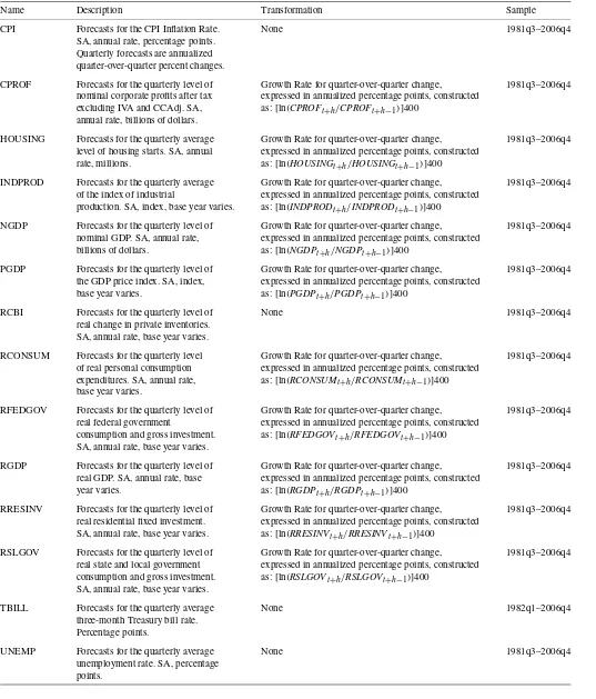
To illustrate the empirical performance of the selection and combination methods, we study one through four-step-ahead survey forecasts of 14 variables that have data going back to 1981 and are covered by the Survey of Professional Forecast-ers. A brief description of these variables is provided in Table2.
4.1 Forecasting Performance
The first 30 forecasts are used to estimate the initial combi-nation weights. The estimation window is then recursively ex-panded up to the end of the sample which gives us 77 fore-casts for h=1 and 74 forecasts for h=4. The
Table 2. Variable descriptions
Name Description Transformation Sample CPI Forecasts for the CPI Inflation Rate. None 1981q3–2006q4
SA, annual rate, percentage points. Quarterly forecasts are annualized quarter-over-quarter percent changes.
CPROF Forecasts for the quarterly level of Growth Rate for quarter-over-quarter change, 1981q3–2006q4 nominal corporate profits after tax expressed in annualized percentage points, constructed
excluding IVA and CCAdj. SA, as:[ln(CPROFt+h/CPROFt+h−1)]400 annual rate, billions of dollars.
HOUSING Forecasts for the quarterly average Growth Rate for quarter-over-quarter change, 1981q3–2006q4 level of housing starts. SA, annual expressed in annualized percentage points, constructed
rate, millions. as:[ln(HOUSINGt+h/HOUSINGt+h−1)]400
INDPROD Forecasts for the quarterly average Growth Rate for quarter-over-quarter change, 1981q3–2006q4 of the index of industrial expressed in annualized percentage points, constructed
production. SA, index, base year varies. as:[ln(INDPRODt+h/INDPRODt+h−1)]400
NGDP Forecasts for the quarterly level of Growth Rate for quarter-over-quarter change, 1981q3–2006q4 nominal GDP. SA, annual rate, expressed in annualized percentage points, constructed
billions of dollars. as:[ln(NGDPt+h/NGDPt+h−1)]400
PGDP Forecasts for the quarterly level of Growth Rate for quarter-over-quarter change, 1981q3–2006q4 the GDP price index. SA, index, expressed in annualized percentage points, constructed
base year varies. as:[ln(PGDPt+h/PGDPt+h−1)]400
RCBI Forecasts for the quarterly level of None 1981q3–2006q4 real change in private inventories.
SA, annual rate, base year varies.
RCONSUM Forecasts for the quarterly level Growth Rate for quarter-over-quarter change, 1981q3–2006q4 of real personal consumption expressed in annualized percentage points, constructed
expenditures. SA, annual rate, as:[ln(RCONSUMt+h/RCONSUMt+h−1)]400
base year varies.
RFEDGOV Forecasts for the quarterly level of Growth Rate for quarter-over-quarter change, 1981q3–2006q4 real federal government expressed in annualized percentage points, constructed
consumption and gross investment. as:[ln(RFEDGOVt+h/RFEDGOVt+h−1)]400
SA, annual rate, base year varies.
RGDP Forecasts for the quarterly level of Growth Rate for quarter-over-quarter change, 1981q3–2006q4 real GDP. SA, annual rate, base expressed in annualized percentage points, constructed
year varies. as:[ln(RGDPt+h/RGDPt+h−1)]400
RRESINV Forecasts for the quarterly level of Growth Rate for quarter-over-quarter change, 1981q3–2006q4 real residential fixed investment. expressed in annualized percentage points, constructed
SA, annual rate, base year varies. as:[ln(RRESINVt+h/RRESINVt+h−1)]400
RSLGOV Forecasts for the quarterly level of Growth Rate for quarter-over-quarter change, 1981q3–2006q4 real state and local government expressed in annualized percentage points, constructed
consumption and gross investment. as:[ln(RSLGOVt+h/RSLGOVt+h−1)]400
SA, annual rate, base year varies.
TBILL Forecasts for the quarterly average None 1982q1–2006q4 three-month Treasury bill rate.
Percentage points.
UNEMP Forecasts for the quarterly average None 1981q3–2006q4 unemployment rate. SA, percentage
points.
based methods estimate the combination weights on the largest common sample and require forecasters to have a minimum of 10 common contiguous observations, although the results are robust to using 20 contiguous observations instead. For the
real-time realized value we follow Corradi, Fernandez, and Swanson (2007) and use first release data.
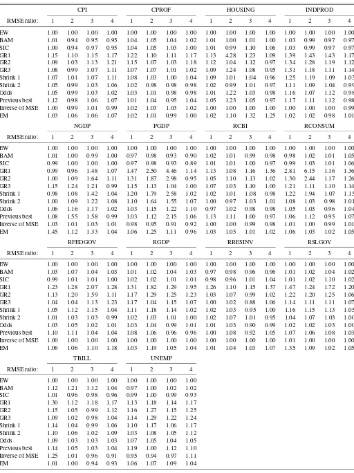
Empirical results in the form of (pseudo real-time) root mean squared error (RMSE) values are presented in Table3. Again
Table 3. Empirical application to forecasts from the survey of professional forecasters
CPI CPROF HOUSING INDPROD
RMSE ratio: 1 2 3 4 1 2 3 4 1 2 3 4 1 2 3 4 EW 1.00 1.00 1.00 1.00 1.00 1.00 1.00 1.00 1.00 1.00 1.00 1.00 1.00 1.00 1.00 1.00 BAM 1.01 0.94 0.95 0.95 1.04 1.05 1.04 1.02 1.01 1.00 1.01 1.00 1.03 0.99 0.97 0.97 SIC 1.00 0.94 0.97 0.95 1.04 1.05 1.03 1.00 1.01 0.99 1.10 1.06 1.03 0.99 0.97 0.97 GR1 1.15 1.10 1.15 1.17 1.22 1.10 1.11 1.17 1.13 4.28 1.23 1.09 1.39 1.43 1.43 1.17 GR2 1.09 1.03 1.13 1.21 1.15 1.07 1.03 1.18 1.12 1.04 1.12 0.97 1.34 1.28 1.19 1.12 GR3 1.08 0.99 1.07 1.11 1.07 1.07 1.01 1.02 1.09 1.24 1.08 0.95 1.31 1.18 1.11 1.14 Shrink 1 1.07 1.01 1.07 1.11 1.08 1.03 1.00 1.04 1.09 1.01 1.04 0.96 1.25 1.19 1.09 1.03 Shrink 2 1.05 0.99 1.03 1.06 1.02 0.98 0.98 0.98 1.02 0.99 1.01 0.97 1.11 1.09 1.04 0.99 Odds 1.05 0.99 1.03 1.02 1.03 1.01 0.98 0.98 1.01 1.22 1.03 0.98 1.16 1.07 1.12 0.98 Previous best 1.12 0.98 1.06 1.07 1.01 1.04 0.95 1.04 1.05 1.23 1.05 0.97 1.17 1.11 1.12 0.98 Inverse of MSE 1.00 0.99 1.01 0.99 1.02 1.03 1.03 1.02 1.00 1.00 1.00 1.00 1.00 1.00 1.00 0.99 EM 1.03 1.06 1.06 1.07 1.02 1.01 0.99 1.00 1.02 1.10 1.32 1.25 1.02 1.02 0.98 1.01
NGDP PGDP RCBI RCONSUM
RMSE ratio: 1 2 3 4 1 2 3 4 1 2 3 4 1 2 3 4 EW 1.00 1.00 1.00 1.00 1.00 1.00 1.00 1.00 1.00 1.00 1.00 1.00 1.00 1.00 1.00 1.00 BAM 1.01 1.00 0.99 1.00 0.97 0.98 0.93 0.90 1.02 1.01 0.99 0.98 0.98 1.02 1.01 1.05 SIC 0.99 1.00 1.00 1.00 0.97 0.98 0.93 0.89 1.01 1.01 1.00 0.97 0.99 1.03 1.01 1.06 GR1 0.99 0.96 1.48 1.07 1.47 2.50 4.46 1.14 1.13 1.08 1.16 1.36 2.81 6.15 1.16 1.36 GR2 1.00 1.09 1.64 1.11 1.31 1.87 2.98 0.95 1.05 1.10 1.13 1.02 1.30 2.44 1.17 1.26 GR3 1.15 1.24 1.21 0.99 1.15 1.13 1.04 1.00 1.07 1.03 1.10 1.00 1.21 1.11 1.10 1.14 Shrink 1 0.98 1.08 1.42 1.04 1.20 1.79 2.58 1.02 1.02 1.01 1.08 0.98 1.22 1.94 1.07 1.15 Shrink 2 1.00 1.09 1.22 1.08 1.10 1.64 1.55 1.07 1.00 0.97 1.03 1.01 1.08 1.03 0.98 1.01 Odds 1.06 1.16 1.17 1.02 1.03 1.15 1.22 1.10 0.97 1.02 0.98 0.98 1.05 1.03 0.96 1.04 Previous best 1.08 1.55 1.58 0.99 1.03 1.12 2.15 1.06 1.13 1.11 1.00 0.97 1.06 1.12 0.95 1.07 Inverse of MSE 1.03 1.01 1.03 1.01 0.98 0.95 0.91 0.92 1.00 1.00 0.99 0.98 1.01 1.00 0.99 1.01 EM 1.45 1.12 1.33 1.04 1.06 1.25 1.11 0.96 1.03 1.05 1.01 1.02 1.06 1.03 1.02 1.05
RFEDGOV RGDP RRESINV RSLGOV
RMSE ratio: 1 2 3 4 1 2 3 4 1 2 3 4 1 2 3 4 EW 1.00 1.00 1.00 1.00 1.00 1.00 1.00 1.00 1.00 1.00 1.00 1.00 1.00 1.00 1.00 1.00 BAM 1.03 1.07 1.04 1.03 1.01 1.02 1.04 1.03 0.97 0.98 0.96 0.96 1.01 1.02 1.04 1.02 SIC 0.99 1.01 1.01 1.00 1.02 1.02 1.01 1.01 0.98 0.96 1.01 1.04 1.01 1.02 1.10 1.02 GR1 1.23 1.28 2.07 1.28 1.31 1.82 1.29 1.95 1.26 1.10 1.15 1.37 1.47 1.24 1.72 1.20 GR2 1.13 1.20 1.59 1.11 1.17 1.29 1.25 1.23 1.03 1.07 0.99 1.02 1.22 1.20 1.25 1.06 GR3 1.04 1.04 1.13 1.23 1.17 1.04 1.15 1.07 1.00 1.02 0.88 1.06 1.14 1.11 1.11 1.07 Shrink 1 1.05 1.12 1.15 1.04 1.11 1.18 1.14 1.02 1.02 1.03 0.95 1.00 1.16 1.15 1.13 1.05 Shrink 2 1.01 1.03 1.03 0.99 1.02 1.03 1.01 1.00 1.02 1.07 1.01 0.95 1.04 1.07 1.03 1.00 Odds 1.03 1.05 1.02 1.01 1.03 1.04 0.99 1.01 1.01 1.03 0.90 0.99 1.02 1.02 1.03 1.00 Previous best 1.10 1.11 1.04 1.04 1.08 1.06 0.96 0.96 1.00 1.08 0.92 1.05 1.07 1.06 1.08 1.03 Inverse of MSE 1.00 1.00 1.00 1.00 1.00 1.00 1.00 1.00 1.00 1.00 1.00 1.00 1.01 1.00 1.00 1.00 EM 1.06 1.06 1.10 1.18 1.03 1.19 1.05 1.04 1.01 1.04 1.03 1.07 1.35 1.09 1.02 1.05
TBILL UNEMP RMSE ratio: 1 2 3 4 1 2 3 4 EW 1.00 1.00 1.00 1.00 1.00 1.00 1.00 1.00 BAM 1.12 1.21 1.12 1.04 0.97 1.00 1.02 1.02 SIC 1.01 0.96 0.98 0.96 0.99 1.00 0.99 0.93 GR1 1.30 1.12 1.18 1.17 1.13 1.18 1.14 1.17 GR2 1.15 1.05 0.99 1.12 1.16 1.27 1.15 1.25 GR3 1.09 1.02 0.98 1.04 1.14 1.29 1.22 1.24 Shrink 1 1.14 1.04 0.99 1.06 1.10 1.17 1.06 1.17 Shrink 2 1.10 1.06 1.02 1.09 1.03 1.08 1.05 1.12 Odds 1.09 1.03 1.03 1.03 1.07 1.05 1.04 1.05 Previous best 1.14 1.05 1.03 1.04 1.19 1.00 1.12 1.10 Inverse of MSE 1.25 1.01 0.96 0.91 0.95 0.94 0.97 1.11 EM 1.01 1.00 0.94 0.93 1.06 1.07 1.09 1.04
NOTE: Root mean squared error (RMSE) ratios are computed using the RMSE of the equal-weighted model (EW) in the denominator. Integers in the table header (1, 2, 3, 4) refer to the forecast horizon in quarters. See Table2for a definition of the series.
we have normalized by the RMSE for the equal-weighted av-erage. In some cases the underlying combination models are nested while in other cases they are not. This makes it difficult to compare the statistical significance of the performance mea-sures which we therefore do not pursue any further.
In common with empirical findings in the literature, the sim-ple equal-weighted forecast turns out to be extraordinarily dif-ficult to beat. For example, the Granger-Ramanathan combina-tions underperform across the board, in some cases by a wide margin. The shrinkage schemes mostly improve upon the least squares combination methods but continue to underperform against the equal-weighted combination. The same conclusion is true for the odds ratio and EM approaches.
Only two methods seem capable of producing better aver-age forecasting performance than the equal-weighted averaver-age, namely the bias-adjusted/SIC method and the inverse of the MSE. The SIC method that selects between the simple and bias-adjusted equal-weighted average does particularly well, producing lower RMSE-values than the equal-weighted fore-cast for close to half of the series including the consumer price index, industrial production, nominal GDP growth, the GDP price deflator, changes in private inventories or resi-dential fixed investments, T-bill rates, and the unemployment rate.
4.2 Bias and Heterogeneity
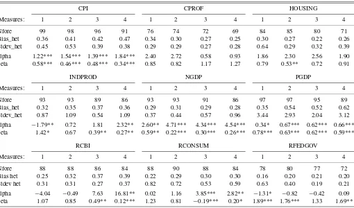
Our earlier analysis suggests that the performance of the equal-weighted mean deteriorates as a result of cross-sectional heterogeneity in forecast precision. To see if this helps ex-plain our empirical findings, Table4reports measures of cross-sectional heterogeneity in the biases along with standard devi-ations of the forecast errors. More specifically, as a measure of
heterogeneity in the biases we report the cross-sectional dard deviation of the forecast biases normalized by the stan-dard deviation of the outcome variable. To measure hetero-geneity in the variance of the forecast errors, we report the cross-sectional standard deviation of forecast error variances, normalized by the variance of the outcome variable. Interest-ingly, cross-sectional heterogeneity in the bias is quite strong for variables such as the CPI and GDP price index where we find that the bias-adjusted mean improves over the simple mean. Similarly, heterogeneity in the variances is strong for variables such as the T-bill rate and the GDP price index, where the bias-adjusted mean again performs well.
Table 4 also shows estimates of α and β from the bias-adjustment regression (7) applied to the full sample. For a ma-jority of the variables, there is strong evidence of biases as
α=0 orβ=1. This is clearly the case for variables such as the consumer and GDP price indexes, nominal GDP growth, res-idential fixed investment, and the T-bill rate where significant biases coincide with good performance of the bias-adjustment method.
4.3 Attrition of Forecasters
Understanding the process whereby forecasters exit from the sample is important. Suppose, for example, that there is a sys-tematic tendency for forecasters who previously produced rel-atively poor forecasts to leave the sample so that only the best forecasters remain. This would suggest focusing mainly on the forecasters with the longest track record. Conversely, if there is only scant evidence that past forecasting performance is related to attrition, then the number of forecasts reported by individual
Table 4. Measures of heterogeneity across forecasters
CPI CPROF HOUSING
Measures: 1 2 3 4 1 2 3 4 1 2 3 4
Nfore 99 98 96 91 76 74 72 69 84 85 80 71 Bias_het 0.36 0.41 0.42 0.47 0.34 0.30 0.27 0.25 0.30 0.27 0.22 0.26 Stdev_het 0.45 0.53 0.39 0.38 0.29 0.29 0.27 0.28 0.64 0.29 0.32 0.39 alpha 1.22*** 1.54*** 1.39*** 1.84*** 2.40 2.72 0.58 0.93 1.86 2.30 2.56 1.90 beta 0.58*** 0.46*** 0.48*** 0.34*** 0.85 0.82 1.17 1.27 0.79 0.53** 0.72 0.91
INDPROD NGDP PGDP
Measures: 1 2 3 4 1 2 3 4 1 2 3 4
Nfore 93 93 89 86 93 93 91 86 97 97 95 89 Bias_het 0.32 0.35 0.37 0.36 0.29 0.31 0.29 0.28 0.35 0.54 0.52 0.62 Stdev_het 0.87 1.09 0.54 1.09 0.37 0.44 0.57 0.96 3.44 2.93 2.04 3.12 alpha −1.79** 0.72 1.81 2.32** 2.60** 4.71*** 4.34*** 4.54*** 0.34* 0.67*** 0.62*** 0.66*** beta 1.42* 0.67 0.39** 0.27** 0.59** 0.22*** 0.30*** 0.26*** 0.78*** 0.63*** 0.62*** 0.59***
RCBI RCONSUM RFEDGOV
Measures: 1 2 3 4 1 2 3 4 1 2 3 4
Nfore 88 88 86 84 88 90 88 84 78 80 77 72 Bias het 0.25 0.32 0.37 0.39 0.22 0.29 0.30 0.30 0.16 0.20 0.21 0.20 Stdev het 0.31 0.31 0.27 0.37 0.82 0.72 0.53 0.59 0.63 0.40 0.19 0.21 alpha −4.04 −0.49 7.63 16.81** 0.02 1.16 3.85*** 2.82** −1.31* −0.82 −0.42 0.09 beta 1.07 0.85 0.49** 0.12*** 1.23 0.81 −0.19*** 0.20* 1.89*** 1.76*** 1.33 1.69**
Table 4. (Continued)
RGDP RRESINV RSLGOV
Measures: 1 2 3 4 1 2 3 4 1 2 3 4
Nfore 96 97 95 89 85 86 83 82 81 81 79 78 Bias_het 0.28 0.30 0.31 0.31 0.30 0.25 0.26 0.31 0.20 0.19 0.23 1.50 Stdev_het 0.33 0.67 0.49 0.68 0.60 0.65 0.53 0.54 0.54 0.99 0.58 180.15 alpha −0.76 1.16 2.89*** 2.21** 1.56* 2.99*** 3.33*** 2.98*** −0.11 0.64 1.18 2.42*** beta 1.34* 0.64 0.07*** 0.32** 1.36** 0.80 0.70* 0.82 1.34 0.87 0.67 0.04***
TBILL UNEMP
Measures: 1 2 3 4 1 2 3 4
Nfore 90 90 88 83 98 98 96 89 Bias_het 0.07 0.11 0.14 0.19 0.07 0.11 0.16 0.18 Stdev_het 0.39 1.35 2.01 1.42 0.11 0.16 0.23 0.29 alpha −0.02 0.28 0.38 0.41 −0.17** −0.20 −0.05 0.26 beta 1.00 0.91*** 0.87*** 0.84*** 1.02 1.02 1.00 0.94
NOTE: Nfore is the number of forecasters with more than 10 forecasts (per variable-horizon). Bias_het is variation in the bias of the Nfore forecasters, computed as the standard deviation in the bias across forecasters divided by the variance of the outcome variable (for the whole sample). Stdev_het is the heterogeneity in the variances, computed as the standard deviation across the Nfore forecasters of the variance (per forecaster) of the forecast error divided by the variance of the outcome variable (for the same periods of the forecasts). Alpha and beta are the parameter estimates of the bias-adjusted mean based on full-sample information. *p<0.10., **p<0.05, ***p<0.01 with alpha equal to zero and beta equal to one under the null hypothesis.
survey participants—or their past forecasting performance—is unlikely to be a good indicator of future performance.
To briefly address this issue we select survey participants with a minimum of 10 reported forecasts. For these we code continued participation as zero and exit as one. For each of the variables in the survey we pool the data across survey partici-pants and estimate probit models using the previous number of forecasts and relative RMSE as regressors. Table5shows when the regressors were significant along with the sign of the coef-ficients in these cases. In many cases the number of previous forecasts is significantly negatively related to the probability of an exit, suggesting that forecasters who have participated in the survey for a long time are less likely to exit. The relative RMSE is significant for only a few of the variables—in many cases with the wrong sign—so the evidence of a link between exits
from the survey and poor past forecasting performance is very weak.
5. CONCLUSION
Real-time combination of survey forecasts requires trading off biases induced by using restricted and suboptimal combi-nation weights against the effect of parameter estimation er-ror arising from the use of less restricted combination meth-ods. This tradeoff changes with the number of forecasts and so helps explain why the entry and exit of forecasters is important to the performance of different combination methods. Attrition in forecast surveys means that the performance of combination methods that require estimating the covariance between the in-dividual forecasts deteriorates relative to that of more robust
Table 5. Results from probit estimation
Variable No. of previous forecasts Relative RMSE CPI 1(−)** 2(−)** 3(−)** 4(−)*
CPROF
HOUSING 1(+)*
INDPROD 2(−)* NGDP
PGDP 3(−)* 1(+)*
RCBI 3(−)** 4(+)*
RCONSUM 2(−)* 4(−)*
RFEDGOV
RGDP 2(−)* 3(−)*
RRESINV 2(−)* 3(−)** 4(−)*
RSLGOV 4(−)*
TBILL 1(−)* 2(−)* 3(−)** 4(−) UNEMP 1(−)* 2(−)** 3(−)** 4(−)*
NOTE: This table indicates significance and signs of coefficients in a probit regression of forecasters’ exit from the survey using the survey participants’ previous number of reported forecasts and their RMSE computed relative to the average RMSE as regressors. * indicates significance at the 10% level; ** indicates significance at the 5% level. (−) represents a negative, while (+) is a positive coefficient estimate.
methods such as equal weighting. We find empirical evidence, however, that the equal-weighted forecast is strongly biased and that a simple bias-adjustment method seems to work well in practice.
ACKNOWLEDGMENTS
We thank Mark Watson (the discussant), two anonymous ref-erees, an associate editor, the editor, Serena Ng, Graham Elliott, and seminar participants at the Real-Time Data Analysis and Methods in Economics conference at the Federal Reserve Bank of Philadelphia. We also thank seminar participants at the 2nd Workshop on Macroeconomic Forecasting, Analysis and Pol-icy with Data Revision at CIRANO, and Banco de México for many helpful comments and suggestions. Andrea San Martín and Gabriel López-Moctezuma provided excellent research as-sistance. Allan Timmermann acknowledges support from CRE-ATES funded by the Danish National Research Foundation. The opinions in this paper are those of the authors and do not nec-essarily reflect the point of view of Banco de México.
[Received August 2007. Revised August 2008.]
REFERENCES
Amato, J. D., and Swanson, N. R. (2001), “The Real Time Predictive Content of Money for Output,”Journal of Monetary Economics, 48, 3–24. Clemen, R. T. (1989), “Combining Forecasts: A Review and Annotated
Bibli-ography,”International Journal of Forecasting, 5, 559–581.
Corradi, V., Fernandez, A., and Swanson, N. R. (2007), “Information in the Revision Process of Real-Time Data,” mimeo, Rutgers.
Croushore, D., and Stark, T. (2001), “A Real-Time Data Set for Macroecono-mists,”Journal of Econometrics, 105, 111–130.
Davies, A., and Lahiri, K. (1995), “A New Framework for Analyzing Three-Dimensional Panel Data,”Journal of Econometrics, 68, 205–227. Elliott, G., Komunjer, I., and Timmermann, A. (2008), “Biases in
Macroeco-nomic Forecasts: Irrationality or Asymmetric Loss?”Journal of European Economic Association, 6, 122–157.
Granger, C. W. J., and Ramanathan, R. (1984), “Improved Methods of Combin-ing Forecasts,”Journal of Forecasting, 3, 197–204.
Graybill, F. A. (1983),Matrices With Applications in Statistics, Belmont, CA: Wadsworth.
Gupta, S., and Wilton, P. C. (1988), “Combination of Economic Forecasts: An Odds-Matrix Approach,”Journal of Business & Economic Statistics, 6, 373–379.
Hong, H., and Kubik, J. D. (2003), “Analyzing the Analysts: Career Concerns and Biased Earnings Forecasts,”Journal of Finance, 58, 313–351. Koopman, S. J. (1993), “Disturbance Smother for State Space Models,”
Bio-metrika, 80, 117–126.
Pesaran, M. H., and Timmermann, A. (2005), “Real Time Econometrics,” Econometric Theory, 21, 212–231.
Schwarz, G. (1978), “Estimating the Dimension of a Model,”The Annals of Statistics, 6, 461–464.
Stock, J. H., and Watson, M. W. (2001), “A Comparison of Linear and Non-linear Univariate Models for Forecasting Macroeconomic Time Series,” in Cointegration, Causality, and Forecasting: A Festschrift in Honour of Clive Granger, eds. R. F. Engle and H. While, New York: Oxford University Press, pp. 1–44.
(2004), “Combination Forecasts of Output Growth in a Seven-Country Data Set,”Journal of Forecasting, 23, 405–430.
Swanson, N. R., and Zeng, T. (2001), “Choosing Among Competing Economet-ric Forecasts: Regression Based Forecast Combination Using Model Selec-tion,”Journal of Forecasting, 20, 425–440.
Timmermann, A. (2006), “Forecast Combinations,” inHandbook of Economic Forecasting, eds. G. Elliott, C. W. J. Granger, and A. Timmermann, Ams-terdam: Elsevier, pp. 135–196.
Watson, M. W., and Engle, R. F. (1983), “Alternative Algorithms for the Es-timation of Dynamic Factor, MIMIC, and Varying Coefficient Regression Models,”Journal of Econometrics, 23, 385–400.
Zarnowitz, V. (1985), “Rational Expectations and Macroeconomic Forecasts,” Journal of Business & Economic Statistics, 3, 293–311.