Full Terms & Conditions of access and use can be found at
http://www.tandfonline.com/action/journalInformation?journalCode=ubes20
Download by: [Universitas Maritim Raja Ali Haji], [UNIVERSITAS MARITIM RAJA ALI HAJI
TANJUNGPINANG, KEPULAUAN RIAU] Date: 11 January 2016, At: 20:48
Journal of Business & Economic Statistics
ISSN: 0735-0015 (Print) 1537-2707 (Online) Journal homepage: http://www.tandfonline.com/loi/ubes20
Tenure Profiles and Efficient Separation in a
Stochastic Productivity Model
I. Sebastian Buhai & Coen N. Teulings
To cite this article: I. Sebastian Buhai & Coen N. Teulings (2014) Tenure Profiles and Efficient Separation in a Stochastic Productivity Model, Journal of Business & Economic Statistics, 32:2, 245-258, DOI: 10.1080/07350015.2013.866568
To link to this article: http://dx.doi.org/10.1080/07350015.2013.866568
View supplementary material
Accepted author version posted online: 18 Dec 2013.
Submit your article to this journal
Article views: 759
View related articles
Tenure Profiles and Efficient Separation
in a Stochastic Productivity Model
I. Sebastian B
UHAIDepartment of Economics, Stockholm University, 106 91 Stockholm, Sweden ([email protected])
Coen N. T
EULINGSFaculty of Economics, University of Cambridge, Cambridge CB3 9DD, United Kingdom and Department of Economics, University of Amsterdam, 1018 Amsterdam, The Netherlands ([email protected])
We develop a theoretical model based on efficient bargaining, where both log outside productivity and log productivity in the current job follow a random walk. This setting allows the application of real option theory. We derive the efficient worker-firm separation rule. We show that wage data from completed job spells are uninformative about the true tenure profile. The model is estimated on the Panel Study of Income Dynamics. It fits the observed distribution of job tenures well. Selection of favorable random walks can account for the concavity in tenure profiles. About 80% of the estimated wage returns to tenure is due to selectivity in the realized outside productivities.
KEY WORDS: Efficient bargaining; Inverse Gaussian; Job tenure; Option theory; Random productivity growth; Wage-tenure profiles.
1. INTRODUCTION
A large empirical literature has looked at wage returns to
job tenure; see Farber (1999) for a survey. The conclusions
of this research still diverge, despite analyzing data from the same countries (mainly the USA) or even the same longitudinal datasets (mostly the Panel Study of Income Dynamics (PSID));
see, for example, Altonji and Shakotko (1987), Abraham and
Farber (1987), Altonji and Williams (1997,2005), Abowd, Kra-marz, and Margolis (1999), Topel (1991), Dustmann and Meghir
(2005), and Buchinsky et al. (2010). Here, we propose a new
direction for this line of research. From a theoretical point of view, large “true” returns to tenure are problematic. Why would a worker separate when she loses her tenure profile by doing so? Hence, separation is likely to be induced by the firm, what we call a layoff. But why would the worker and the firm prefer separation above renegotiation? Although some models offer explanations for this, the size of the reported wage returns to tenure remains puzzling.
This article addresses explicitly whether the data are consis-tent with efficient separations, by modeling simultaneously the evolution of wages and the distribution of job tenures. The model explains the correlation between wages and job tenure from the
random evolution of both the job’sinside productivityand the
outside productivity, that is, the productivity in the best alterna-tive job. Separation occurs when the value of the inside produc-tivity falls below the outside producproduc-tivity. By some form of bar-gaining, log wages are a linear combination of the in- and outside log productivity. Then, wages and tenure are correlated because only those jobs survive for which the inside productivity remains above the outside productivity. There is no such thing as “the re-turn to tenure” in this model. In some jobs, wages go up because the inside productivity evolves favorably. In other jobs wages go down for mutatis mutandis the same reason. However, these jobs are gradually eliminated from the stock of ongoing job spells be-cause there are no options left for mutually gainful renegotiation.
We assume both log inside and outside productivities to fol-low Brownian motions. Since log wage is a linear combination of them, it also follows a random walk. The evolution of an in-dividual’s log wage is indeed reasonably described by a random walk with transitory shocks, see, for example, Abowd and Card (1989) or Meghir and Pistaferri (2004). What we call the return to tenure is then the difference between the drifts of the log wage and of the log outside productivity. Starting a job requires an irreversible specific investment, which is lost upon separation. The combination of irreversibility and productivity following a random walk implies that we can apply the theory of real
options; see, for example, Dixit (1989) and Dixit and Pyndick
(1994), and compare Teulings and Van der Ende (2000). The
predicted hazard rates of this model are well in line with the empirical distribution of job exits. From the distribution of job tenures we are able to estimate the surplus of the inside over the outside productivity, and the drift of this surplus. We obtain a positive drift, indicating that some 10% of all jobs will end only by retirement. We use these results to compute the evolution of the expected surplus, conditioning on both the date of job start and of job termination, an empirical strategy explored earlier by Abraham and Farber (1987). Our model predicts this variable to be correlated with the evolution of wages.
We obtain the following results. First, a closed form expres-sion is computed for the expected surplus in completed job spells. We show this not to depend on the drift of the surplus. The evolution of wages in completed spells is thus uninforma-tive on the return to tenure in this model, since the effect of the drift is exactly offset by the selection due to the elimination of
© 2014American Statistical Association Journal of Business & Economic Statistics
April 2014, Vol. 32, No. 2 DOI:10.1080/07350015.2013.866568
Color versions of one or more of the figures in the article can be found online atwww.tandfonline.com/r/jbes.
245
bad matches. This is an unexpected conclusion, given that so many studies have tried to identify the return to tenure from this type of data. Second, we show that our model can easily explain the observed concavity in the tenure profile from the selection effect. Selection is much more important than the drift. Third, we show that the selection effect is driven by the selectivity in the outside, as opposed to the inside, productivity. Workers switch jobs mainly when the outside productivity is high, not so much when the inside productivity is low. Selectivity in the outside option accounts for 50%–80% of the tenure profile. This source of selectivity usually receives little attention in the literature on wage-tenure profiles, though it figures in models of equilibrium
on-the-job-search, for example, Burdett and Mortensen (1998).
In this search literature, closest to us are “persistent earnings
dynamics” studies by Postel-Vinay and Turon (2010) and Low,
Meghir, and Pistaferri (2010); unlike them, our wage process
does not require nesting within models of search, or classic au-toregressive moving average (ARMA) decomposition. Finally, our estimation results suggest downward rigidity in wages, as
discussed, for example, by Beaudry and DiNardo (1991). This
downward rigidity does not fit the efficient bargaining hypoth-esis. Our estimates also provide evidence of excess variance in wages for job movers, implying failure of our Walrasian market assumption for outside offers.
The article is structured as follows: the model is discussed in Section2, the identification and the estimation are set out in Section3, and the empirical analysis is presented in Section4.
2. THE RANDOM PRODUCTIVITY GROWTH MODEL
2.1 Model Assumption
Consider a labor market in continuous time, where both work-ers and firms are risk neutral. We focus on a single cohort of
homogenous workers. We normalize our measure of timetsuch
that it is also equal to the workers’ experience. There is no disutility of effort, so that the workers’ utility depends on their expected lifetime income only. Each firm offers a single job, of
which the job specific productivityPt evolves according to a
geometric Brownian motion with drift. At the moment a worker is hired for a vacant job, a specific investment has to be made, which is partly paid by the firm and partly by the worker, and which is irreversibly lost upon separation between the worker and the firm. However, the firm retains the option value on the vacancy: it can hire a new worker at any future time, provided that the cost of the specific investment is paid again. The in-vestment is verifiable. There is no search cost involved from either party in finding a new job: an unemployed worker can just pick the most attractive vacancy that is available at that time, at zero cost. LetRt be the return on this vacancy, net of
the cost of investment;Rtis exogenous in this model. LikePt,
it evolves according to a geometric Brownian motion with drift. Both workers and firms are perfectly informed about the current values ofPtandRt, but their future evolution is unknown. The
value of the specific investments for a job starting at timetis
RtI. One can think ofI as the cost of investment measured in
units of labor time and ofRt as the price of one unit at timet.
Using lower cases to denote the logs of the corresponding upper cases, the law of motion ofptandrt, fort > s, is characterized
Sinceμr is the drift in the log outside option of the worker, it
can be interpreted as the sum of the return to experience and the secular growth in real wages due to technological progress. The worker and the firm bargain over the surplus of the productivity
of the job above the shadow price of a worker,Pt−Rt. This
bargaining is efficient: as long as there is a surplus, the worker and the firm will agree on a sharing rule. In the empirical appli-cation in Sections3and4,Iandμp will be allowed to depend
on personal characteristics. For the derivation of the model this dependence on personal characteristics can be ignored.
2.2 Value of a Job and a Vacancy
Three assumptions made above greatly simplify the analysis. (i) The risk neutrality of both players implies that the alloca-tion of risk is irrelevant: only expected values matter. (ii) The verifiability of investment implies that there are no hold up problems: the distribution of future surplusesPt−Rt,t > s, is
irrelevant for the timing of the investment decision, since the
cost of the specific investmentRsI can always be shared
be-tween the worker and the firm according to their share in future surpluses. Hence, the investment decision will maximize the joint expected surplus of the worker and the firm. (iii) Efficient bargaining implies that separation decisions will also maximize the joint expected surplus. Hence, separation occurs at mutual consent when there are no gains from trade left. Quits and lay-offs are therefore observationally equivalent, as in McLaughlin (1991). For convenience, we shall refer to a separation as the firm firing the worker, though it can be both a quit and a layoff. Given these assumptions, wage setting and separation decisions can be analyzed separately: in the spirit of the Coase theorem, hiring and firing decisions maximize the joint expected surplus, regardless of its distribution.
First, we analyze hiring and firing. Since hiring requires an irreversible investment, while firing is an irreversible disinvest-ment, both can be analyzed using real option theory; see, for
example, Dixit and Pindyck (1994). The easiest way to analyze
this problem is to assume that workers always get paid their
shadow priceRt. Then, hiring and firing simply maximize the
expected value of the firm. LetV(pt, rt) andJ(pt, rt) be the
ex-pected present value of a vacancy and, respectively, of a job, as functions ofptandrt. Applying Ito’s lemma, the Bellman
equa-tions for both value funcequa-tions read, compare Dixit and Pindyck (1994, pp. 140–141):
where we leave out the arguments ofJ(·) andV(·) for
con-venience, and where ρ denotes the interest rate. The term
exp(pt)−exp(rt) in the first equation is the value of current
output minus the wage of the worker; the other terms capture the wealth effects due to changes in the state variablesptandrt:
the first-order derivatives capture the effect of the drift in both state variables, the second-order derivatives capture the effect of their variance. For optimal hiring and firing, value matching and smooth pasting conditions should be satisfied:
J(pS, rS)=V(pS, rS)+exp(rS)I, V (pT, rT)=J(pT, rT)
Jp(pS, rS)=Vp(pS, rS) , Vp(pT, rT)=Jp(pT, rT), (3)
whereSis the moment of hiring andTis the moment of firing.
The first two conditions are the value matching conditions for hiring and firing, respectively, the second pair of conditions is the smooth pasting conditions forpt; the smooth pasting conditions
forrt are redundant. Value matching conditions impose value
equality at the moment of hiring and firing; on top of that, smooth
pasting conditions impose that slight variations in pt should
not affect the value equality, since hiring and firing decisions are irreversible. Hence, a decision maker should not regret her decision after slight variations inpt. The above conditions and
the Bellman Equations (2) jointly determineJ(·) andV(·).
V(·). The proposition follows directly from substitution of
these expressions in Equations (2) and (3).
The factorρ−μr−12σr2is a modified discount rate, which
accounts for the fact that future revenues are discounted at rate
ρ, but increase in expectation at rateμr+12σr2due to the drift
and the variance ofRt. The hiring and separation rules depend
therefore purely on bt: a vacancy should be filled at the first
timet that bt =bS, a worker should be fired from the job at
the first timetthatbt=bT. This proposition characterizes the
decision problem of the firm by two second-order differential equations, four boundary conditions, and two decision param-eters,bS andbT, see Dixit and Pindyck (1994, chap. 5.1 and 5.2), to whom we refer for the subsequent arguments. The two differential equations have an analytical solution. These solu-tions yield four constants of integration. Two of these constants
have to be zero due to transversality conditions. The constants of integration reflect the option value for the firm of hiring and firing a worker. The option value of hiring converges to zero whenbt →0, while the option value of firing converges to zero
whenbt→ ∞. These constraints can only be satisfied by
set-ting two constants of integration equal to zero. Hence, the four
boundary conditions determine four unknown parameters:bS,
bT, and the two remaining constants of integration. One can
provebT <0< bS. Hence, at the moment of hiring,PS > RS
because the firm has to recoup the cost of investment and be-cause the investment is irreversible, so that the firm loses the
option value of delaying hires, while in the meantimebt might
fall belowbSat a later point in time. Similarly, at the moment
of firing,PT < RT because the firm accepts some losses before
firing the worker, since by doing so it loses the option value of firing the worker at a later point in time.
2.3 Job Tenure Distribution
The duration of a job spell is a stochastic variable, equal to the time it takes the random variablebtto travel down frombS
tobT. The standard deviation ofb
t is unidentified in this model
because, for any timet, we observe only whether the spell is still incomplete, implyingbt−bT >0 ever since the start of the job
spell. We can therefore normalize all parameters byσ. For each
job spell, we defineτ ≡t−S, withτ ≥0, and, respectively,
≡T −S, with >0;τ is the incomplete tenure, whileis
the completed tenure of that job spell. Define
τ ≡
Thus,τ is a Brownian motion with driftπ and unit variance
per unit time. By construction,0 =and=0.can be
shown to be an implicit function of the model’s structural pa-rameters,I ≡H(, μ, ), withH(·)>0. Hence, we treat the
parameteras the parameter of interest. If desired, the
under-lying structural parameterI can be recovered via the function
H(, μ, ).
The completed job spellis determined by the time it takes
τ to pass the barrierτ =0 for the first time. This process
satisfies the “First Passage Time” distribution, which has been applied previously by Lancaster (1972) for modeling strike dura-tions, and by Whitmore (1979) for job spells. The unconditional
density ofτ =ωreads
where φ(·) is the standard normal pdf. However, a job spell
is completed if and only if t has not been negative for any
t ∈[0, τ]. Hence, we are interested in the density ofτ
con-ditional ont >0,∀t ∈[0, τ]. For this conditioning, we can
apply the Reflection Principle, first discussed by Feller (1968):
there is a one-to-one correspondence between trajectories ofτ
from toω, which have crossed the barrierτ =0 at least
once, and trajectories ofτ from−toω. These trajectories
should therefore be subtracted to obtain the conditional density ofτ. Defineg(ω, τ)≡Pr(τ =ω∧ > τ). It satisfies, see,
0.5 1 1.5 2
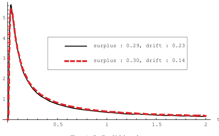
surplus : 0.30, drift : 0.14 surplus : 0.29, drift : 0.23
Figure 1. Predicted job hazards.
for example, Kijima (2003, pp. 185–187):
g(ω, τ)
where φ(.) is the standard normal density function. The first term in square brackets is the unconditional density; the second is the effect of the conditioning. By the Reflection Principle, the latter is the density of trajectories ofτfrom−toω. The
factore−2πcorrects for the differential effect of the drift on the density for upward and downward trajectories. By integrating outω, we get the cumulative distribution of jobs surviving atτ,
F(τ)=Pr( > τ):
where(.) is the standard normal cdf. This expression is iden-tical to Whitmore (1979, eq. (2)). The distribution ofis there-fore fully specified by two parameters, the initial distance from
the separation threshold , and the driftπ. Hence, andπ
can be identified from data on job tenures, while the
parame-terσ cannot. The corresponding density function is minus the
derivative ofF(τ) with respect toτ: declining monotonically to 0 for a positive driftπ >0, or to
1/
2π2forπ <0. Farber (1994) and Horowitz and Lee (2002)
had documented this hump-shaped pattern using National Lon-gitudinal Survey of Youth (NLSY) data. A positive driftπ >0 implies that some fraction of the started jobs will never end.
This fraction is equal to the survivor function (8) evaluated at
τ → ∞, hence to 1−e−2π.
values of the observed and unobserved worker characteristics,
see Section 3, Table 2. In both cases the peak is reached at
τ ≃0.04 years. Sinceπ >0, the hazard rate converges to zero and a positive fraction of the jobs, about 10%, will never end.
2.4 Tenure Profile in Wages
2.4.1 Sharing Rule of Surpluses and Wages. We extend this model with an explicit sharing rule of surpluses during the course of the job spell. Ideally, we would derive this sharing rule from an explicit bargaining game, such as Nash bargaining. For the sake of convenience, we use a simpler approach, imposing the log linearity of the sharing rule a priori, and deriving the intercept of that rule from the assumption of efficient bargaining. According to this rule, the worker’s log wagewtsatisfies
wt =rt+β(bt−bT)+ut =rt+σ τ+ut, (10)
where σ ≡βσ. We assume ut is an iid random variable
dis-tributedN(0, σ2
u): this specification of wages as following a
ran-dom walk,τ, with a transitory shock MA(1),ut, is broadly
con-sistent with a large number of studies on the dynamics of wages;
see, for example, MaCurdy (1982), Abowd and Card (1989),
Topel and Ward (1992), and Meghir and Pistaferri (2004). The parameterβcan be interpreted as the worker’s bargaining power. Ifβ =0, the wage is equal to the worker’s outside productivity
Rt, while ifβ=1, the wage is her inside productivityPt. The
transitory error can be interpreted as either measurement error in wages; see, for example, Meghir and Pistaferri (2004), or as short run fluctuations that do not affect the long run payoff of the specific investmentIin the current job. In either interpretation,
these shocks do not affect the optimizing behavior of agents regarding job change.
2.4.2 Selectivity in Tenure Profiles. Equation (10) implies that log wages within a job follow a Brownian motion with driftμr+σ π; μr is the sum of the return to experience and
the secular growth of real wages due to technological progress;
σ π is the deterministic part of the tenure profile. Were the
realizations of τ independent of the completed job tenure
,σ π could be estimated easily. However, in completed job
spells,τ is correlated withfor three reasons: (i)0=,
(ii) =0, and (iii) t >0,∀t,0≤t < . For the sake
of brevity, we refer to this information set asA(). Mutatis
mutandis, the same applies to incomplete spells. Let be the
incomplete tenure at the last date for which data are available.
Again, there are three pieces of information: (i) 0=,
(ii) > , and hence (iii)t >0,∀t,0≤t ≤. We refer to
this second information set asB().
Proposition 2. Letm(τ)≡ −τ. E[τ|A()] and its
deriva-on the tenure profile in wages, σ π; see also Van der Ende
(1997). Hence, conditional on the model that we specified, the evolution of wages in completed job spells does not provide any information whatsoever on the tenure profile in wages. Given the many articles that have tried to estimate tenure profiles from data on completed job spells, this is a very surprising conclusion. The intuition for this result is that an increase inσ π has two offsetting effects onE[τ|A()]. On the one hand, it raises
the deterministic part of the tenure profile, so that the change in
the unconditional expectationE[τ] goes up. On the other
hand, it makes separation a less likely event, so that the condition
A() becomes more informative: the higher isσ π, the more
unfavorable the evolution of the nondeterministic part ofτ
must have been to warrant a separation. Hence, the deterministic part of the tenure profile does affect the job separation rate, but it does not affect the evolution of wages, conditional on the
moment of separation.
The conclusion above depends crucially on the assumption of efficient bargaining. Ignoring the impact of temporary shocks
ut, this assumption dictates that the evolution of wages over a
job spell satisfies
(wS−rS)−(wT−rT)=σ ,
see Equation (10). The difference between the starting and the terminal value of this log relative wage is equal to the worker’s
share in the surplus due the specific investment in the job,σ . Hence, irrespective of the steepness of the tenure profile σ π,
or the job spell length , log relative wages decline by σ
over the duration of a completed job spell. However, π can
be estimated from the tenure distribution. Efficient bargaining implies that this distribution is informative on the tenure profile, since under efficient bargaining a higher tenure profile means that jobs will survive longer. From this perspective, data on the tenure distribution are more informative on the return to tenure than data on wages.
The second relationship of Proposition 2 says that the initial slope of E[τ|A()] is negative for short spells, < 2, even
when the drift is positive,π >0. For these spells, E[τ|A()]
must decline immediately for =0. The third expression
shows that the expected surplus declines infinitely fast just be-fore separation. This is consistent with empirical evidence by Jacobson, LaLonde, and Sullivan (1993) on the decline in rela-tive wages in the period just before firing. The final expression shows that the second derivative is always negative. Hence, E[τ|A()] is concave inτ; it is monotonically decreasing for
short spells < 2 and it is hump shaped for longer spells.
Contrary to the case of completed spells, there is no explicit ex-pression for E[τ|B()]. Hence, we use numerical integration
in this case, see the Appendix.
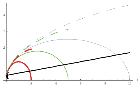
Figure 2 plots the evolution of E[τ|·] for =0.30 and π =0.14, for both completed spells (continuous lines) and
in-complete spells (dashed lines), with durations and,
respec-tively,in{0.1, 2,5,10}. Moreover, the straight line shows the drift:+π τ. With respect to completed spells, E[τ|A()]
is monotonically decreasing for≤0.1 year, and concave for
larger. The top of the profile is increasing in, showing the importance of conditioning on the eventual tenure. With respect to incomplete spells, E[τ|B()] is increasing in. The
rea-son is that higher values of imply greater selectivity, since
> . Trajectories are strongly concave, indicating that se-lection plays an important role. This can explain the observed concavity of tenure profiles in log wages: the underlying pro-file might be linear, with the observed concavity simply due to selection. The trajectories for both completed and incomplete spells are far above the deterministic part, except for the final year(s) before separation: selection dominates.
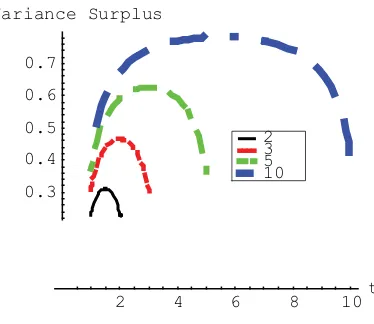
The same analysis can be done for the second moment of
τ. Expressions for var[τ|A()] and var[τ|B()] can
Figure 2. Expected surplus in completed and incomplete spells.
2 4 6 8 10t
Figure 3. Variance surplus in completed spells.
be found in the Appendix. In the absence of conditionA(),
var[τ] would be equal to unity, see definition (6). However,
conditionsA() andB() introduce selectivity in the trajec-tories of the random walk.
This selectivity reduces the variance, as shown inFigure 3.
The variance is low initially, because the positive constraintτ
over the course of a job spell is quite informative, and 0 is
small. The same argument applies toward the end of completed
spells, since =0 by construction. For longer spells, the
variance converges to unity in the middle part of the spell.
2.5 A Reinterpretation of the Wage Equation
The implications of our analysis on the selectivity in tenure
profiles surface most clearly when we rewrite Equation (10),
benefiting from a decomposition of the random variables [pt, rt] into two orthogonal components [bt, zt]. We
nor-malizeztsuch that its marginal effect onrtandptis equal
to unity:
This decomposition satisfies the constraint pt−rt =bt
imposed by Equation (4).
Since separation decisions are determined by the evolution
of bt, and since bt and zt are uncorrelated, selectivity
affects bt, but not zt. Combining these definitions with
Equation (10) yields
wt =zt+γ βbt+ut =zt+γ σ τ+ut. (12)
The parameterγ is a reflection of the correlation between the
match surplus and the reservation wage. In the one extreme case,
γ =0, we can writept =rt+bt, where the right-hand
side variables are uncorrelated. Thenrt reflects the evolution
of the general human capital of the worker, which evolves inde-pendently of the value of the specific capital in the present job,
bt. Hence, the duration of the actual job is fully determined
by its own (mis)fortune. Though the distinction between quits and layoffs makes little sense in this model, separations look like layoffs in this case: the firm fires the worker since she is
no longer productive. In the opposite extreme case,γ =1 , we
can writert =pt−bt, again with uncorrelated right-hand
side variables. Nowptreflects the evolution of the general
hu-man capital of the worker;btreflects the specific evolution of
outside opportunities, for example, new technologies emerging in other firms. Separations look like quits in this case: the worker quits because she can get a better job elsewhere. In this case, the selectivity of job relocation is not so much that of the type “only good jobs survive outside offers,” but more of the type “only good outside offers kill the job.”
3. ESTIMATION METHODOLOGY
3.1 Identification
The model has in total eight structural parameters: two drift parametersμ, three (co)variances, the initial surplus, the
worker’s bargaining power β, and the variance of the
transi-tory shock σu2. As shown in Section 2.3, the distribution of completed job tenures is fully determined by two parameters,
π and , while wages are characterized by five parameters,
σ , γ , μz, σz, and σu. Hence, one can never hope to identify
more than seven parameters, two from the tenure distribution, and five from wages. The model is therefore identified up to
one degree of freedom. Equation (12) reveals why this is the
case. Only the productσ ≡βσ shows up, not its componentsβ
andσ. Data on either the cost of necessary investmentIor the productivityptwould resolve this underidentification, offering
direct information onσ. Then,βcould be established asσ /σ. However, neither type of data is available here.
We assumeandμp to depend on personal characteristics.
We allow for both observed and unobserved characteristics. As
observable we enter experience at the moment of job startS,
measured in deviation from its sample mean. Since we have longitudinal data with multiple job spells per individual, we
can account for random worker effects;eandeπare normally
distributed, uncorrelated, random worker effects with zero mean
and standard deviationsσandσπ, respectively. We apply an
exponential specification forsince this parameter is positive
by definition:
=exp (ω0+ω1S+e) (13)
π =π0+π1S+eπ μz=μ0+γ σ(π1S+eπ).
Since experience at job startS enters the analysis in deviation from its mean across jobs, the interceptsω0, π0,andμ0can be
interpreted as the mean value for ln, π, andμz, respectively.
Our estimation strategy uses the recursive feature of our model. The parametersω0,1, π0,1, σ, andσπare estimable from
job spell data. Estimates of these parameters are then used to cal-culate conditional expectations and variances of the change in
surplusτ, in both completed and incomplete job spells. The
resulting expressions are subsequently employed in the analysis of wage dynamics. Below, we first show howω0,1, π0,1, σ, and
σπ can be estimated by maximum likelihood from the tenure
distribution; next, we derive a set of moment conditions for estimatingμ0, σz2, σ , γ, andσu2from the evolution of wages.
3.2 Maximum Likelihood Estimation ofω0,1andπ0,1
The contribution to the log-likelihood function for an indi-vidual reads
able, taking the valuedj =1 if the job spell is completed and
dj =0 otherwise. There are two reasons why we need to make
amendments to this likelihood function.
First, we could restrict the estimation to job spells starting within the observation range of our dataset. However, then we would not consider any of the jobs started before they were first reported in the data; by construction, this would limit the max-imum completed tenure to the maxmax-imum time span, 17 years,
covered by our PSID sample, see Section4. Since long tenures
contain relevant information, we want to include also the spells ongoing at the start of the sample. Since we observe these spells only conditional on the fact that they have lasted till the start of the sample period, we correct the initial likelihood function for this conditioning:
whereτ1is the tenure in the job at the start of its observation in
the PSID (for whichj =1).
Second, since the PSID stock samples data at yearly intervals, job spells completed in less than a year are underreported. We know the elapsed tenure in months at the first moment a job spell is observed, by a retrospective question, but do not know whether there has been another job spell between the job observed a year ago and the current job. Since the hazard rate implied by our model is hump shaped, with the hump likely to be within the first year, see Farber (1994), we are likely to overestimate
and π, as we miss part of the short tenures in our data.
One solution to this problem is to apply a similar conditioning as in Equation (15), whereτj is the initial tenure at the first
moment the job is observed. However, this approach does not use the distribution ofτj’s itself. We can use this distribution
if we are prepared to make the additional assumption that the starting date of job spells is distributed uniformly over the first year. Then, the densityq(·) of initial dates of spells that started throughout the year and are still incomplete at the end of the year satisfies:q(τ)=F(τ)/01F(x)dx. The total contribution to
the likelihood of a spell with initial tenureτ and completed
tenureis thus:
Hence, the final log-likelihood, accounting both for the jobs started before their first reporting in the PSID and for the under-reporting of spells shorter than a year due to the stock sampling scheme of the data, can be written as
logL=ln
whereI(y) is the indicator function, taking value 1 ifyis true and 0 otherwise. We estimate the log-likelihood function in (16) by simulated maximum likelihood (SML). We report estimates for two samples, a “small” one including only jobs starting within the observation range of our PSID extract, and a “large” one including also the jobs ongoing at the start of the dataset.
3.3 Moment Conditions for Wage Dynamics
Using the maximum likelihood estimates of the parameters
ω0,1, π0,1, σ, andσπ, we can calculate the conditional
expec-tations and variances ofτ. These expressions are then used
for the estimation of the parametersσ , γ , μ0, σz,andσuby a
method of moments, using data on wage changes. The condi-tions for the first two moments can be derived by substitution of Equation (13) in Equation (12), and taking the expectation and the variance. This yields the following system of equations:
wt =μ0+γ σ π1S+γ σEτ+εt (17)
script ∗ indicates the log wage or, respectively, change
in surplus just before separation from the previous job,
and where Eτ≡ E[τ|A(), B()], and varτ≡
var[τ|A(), B()]. We impose no constraints upon the
covariance matrix of these five error terms. In the third and fourth lines, we use var[wt]=E[wt2]−E[wt]2, where we
substitute E[wt] with the deterministic part of the right-hand
side in the first, and, respectively, the second equation. The first two equations are the conditions for the first moment, for within and between job spell wage changes, respectively. The second pair of equations are the conditions for the second moment, again for within and between job spell wage changes. The final moment condition is the covariance between subsequent wage changes due to the transitory shocksut.
The system of Equations (17) is characterized by additive
disturbances and nonlinear cross-equation restrictions in the parameters. It can be estimated by feasible generalized nonlinear least squares (FGNLS). Since we useω0,1, π0,1, σ, andσπ as
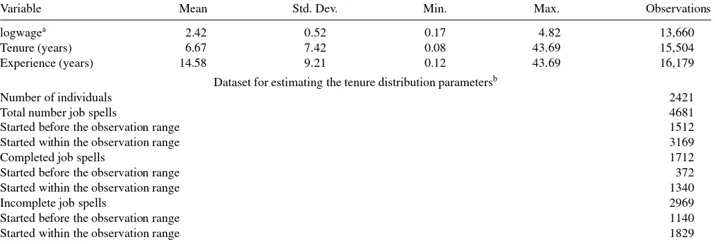
Table 1. Summary statistics
Variable Mean Std. Dev. Min. Max. Observations
logwagea 2.42 0.52 0.17 4.82 13,660
Tenure (years) 6.67 7.42 0.08 43.69 15,504
Experience (years) 14.58 9.21 0.12 43.69 16,179
Dataset for estimating the tenure distribution parametersb
Number of individuals 2421
Total number job spells 4681
Started before the observation range 1512
Started within the observation range 3169
Completed job spells 1712
Started before the observation range 372
Started within the observation range 1340
Incomplete job spells 2969
Started before the observation range 1140
Started within the observation range 1829
NOTES:aReported average hourly wage, deflated using the implicit price deflator with 1982 base year. bSubset of the data summarized in the top panel, keeping one observation for each job spell.
estimated by SML in the first step analysis, see Section 3.2,
in this second step we need to correct the standard errors of the FGNLS estimates for the estimation error introduced by the SML. We follow the methodology outlined by, for example,
Murphy and Topel (1985). Details on the FGNLS estimation
and on the adjustment of the standard errors of the FGNLS estimates are relegated to our web appendix.
4. EMPIRICAL ANALYSIS
4.1 Data
We use as data a PSID extract of 18 waves, covering the years 1975 through 1992. Our model does not work well when employed people consider other alternatives than switching to another job, such as retirement, leaving the labor force, or taking up full time education. The availability of these other alternatives yields two problems. First, we do not observe the reservation wage at the point of separation when people do not accept an-other job. Second, with only one alternative to the present job, the decision problem is simply whether a particular indicator switches signs. With more alternatives, that choice process be-comes far more complicated. Therefore, we restrict the sample to people who do not switch in and out the labor force regularly, and for whom retirement is not a relevant option: white male heads of household, with more than 12 years of education, and less than 60 years of age. Furthermore, we restrict the sample to those individuals that were employed, temporarily laid off, or unemployed at the time of the survey. We exclude people from Alaska or Hawaii. Finally, we discard all observations on unionized jobs. Through these initial data selection procedures we discard in total 10,351 observations from the original dataset used by Altonji and Williams (1999).
For the analysis of wage dynamics, observations for which wages are missing (2404 obs.) or topcoded (254 obs.) are
deleted, as well as observations for which |wt|>0.50
(276 obs.). This leaves a total of 8082 observations on within-job wage changes, and 462 observations on between-within-job wage
changes. Wages are deflated by the implicit price deflator, using 1982 as base year, as in Altonji and Williams (1999).
Table 1presents summary statistics of the data. Tenure and experience measures are constructed by Altonji and Williams
(1999). Observations with missing wage information are
in-cluded in the tenure distribution analysis. One can distinguish four types of job spells. Apart from the distinction between completed and incomplete spells (right censoring), one can also make a distinction between spells that start before the time span covered by our data and spells that start afterward. The lower half of the summary statistics table informs on the number of spells for each of these four types.
4.2 The Parameters of the Tenure Distribution
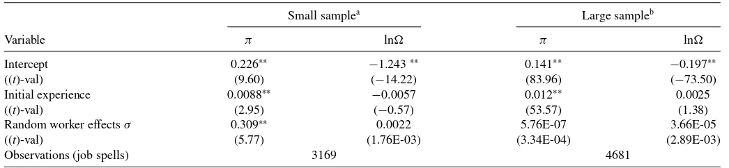
Estimation results for the tenure distribution analysis, see Equation (16) and parameter specification (13), are presented in Table 2. Theoretically, the results for the “large sample,” including the jobs ongoing at the start date of the PSID sample, and for the “small sample,” excluding those jobs, should be identical. Both job exit hazards look indeed almost identical for
the estimated mean values of lnandπ, see againFigure 1,
with the peak in the hazard somewhat lower for the large sample.
Inspecting the estimates inTable 2yields the same conclusion.
The intercepts and the coefficients for experience at job start are very similar for both samples. The positive effect of expe-rience on the drift is consistent with the idea that workers start their career with some initial job hopping, before settling down in a job that fits their comparative advantages best. The intercept forπis positive and large for both samples. In both cases, there
are hardly observations for whichπ is negative. This implies
that a fraction of the job spells will last until the retirement of the worker. The fraction of jobs that never end is about 10%,
computed for the mean values of lnandπ.
An interesting observation is that while we find unobserved random worker effects for the small sample, we do not find any for the large sample. The same result is found for a slightly different specification of the model, see Teulings and Van der
Table 2. SML estimates tenure distribution parameters Equation (16)
Small samplea Large sampleb
Variable π ln π ln
Intercept 0.226∗∗ −1.243∗∗ 0.141∗∗ −0.197∗∗
((t)-val) (9.60) (−14.22) (83.96) (−73.50)
Initial experience 0.0088∗∗ −0.0057 0.012∗∗ 0.0025
((t)-val) (2.95) (−0.57) (53.57) (1.38)
Random worker effectsσ 0.309∗∗ 0.0022 5.76E-07 3.66E-05
((t)-val) (5.77) (1.76E-03) (3.34E-04) (2.89E-03)
Observations (job spells) 3169 4681
NOTES: Significance levels:∗∗: 1%. Statisticalt-values in parentheses under estimated coefficients.
aSmall sample=sample of job spells starting within the observation range of the PSID sample. bLarge sample=sample of all job spells, including those ongoing at the PSID sample start.
All covariates are taken in deviations from their means over jobs.
Ende (2000), or for slightly different samples or specifications that we estimated, but do not report in the article (i.e., including unionized jobs, or including education as an explanatory vari-able). The main difference between the samples is that the large one contains more long job spells, since it includes ongoing spells at the start of the PSID extract. As pointed out earlier, estimates for the two samples should be identical; since this is not the case, we suspect some form of misspecification of the empirical model. Given that some prior studies have estimated considerable unobserved heterogeneity in the PSID, see Brown-ing, Ejrnaes, and Alvarez (2010), this misspecification must be related to the sample containing the long job spells. What form of misspecification of the hazard rate for long job durations might explain our result? Part of the jobs last until retirement. Since our model does not describe the outside option of leaving the market due to retirement, and we therefore exclude workers above 60, a share of the jobs will never end according to this model. This explains why we find the drift to be positive. As discussed in Section2.3, a positive drift implies the hazard rate to be steadily declining to 0. Heterogeneity in the drift would strengthen this decline. Due to selection, the sample of surviving job spells will be increasingly made up of workers with a high drift. Hence, the hazard rate will decline more rapidly when there is heterogeneity in the drift than when there is not. The data do not support this rapid decline in the hazard, hence the estimated zero variance of the random worker effect.
From this perspective, it is pertinent to compare our model
with Jovanovic’s (1979) Bayesian learning model, where the
firm learns about the productivity of a match by subsequent realizations of its output. That model has a stochastic struc-ture similar to the model considered here. New information about the quality of a match is orthogonal to the previously col-lected information. However, as times goes by, the quality of the firm’s information set improves and new information will have a smaller impact. Hence, the hazard rate in learning mod-els declines much faster than in our model. The data strongly reject this rapid decline. Our model comes a long way in ex-plaining the slow decline in the hazard rate for long job spells. However, the absence of unobserved heterogeneity in the drift suggests that the actual decline is even slower than our model predicts.
Since the long spells started before the first wave of our PSID sample contain crucial information, we focus on the results for
andπ obtained from the full sample of job spells for the
subsequent wage dynamics analysis.
4.3 Wage Dynamics
The FGNLS estimation results of system (17) are reported in
Table 3. The equations in (17) impose a linear experience profile. However, the model can be easily extended with a concave experience profile, since this affects rt andpt equally. We do
so throughout the subsequent analysis. As stated in Section3.3, since we make use of the earlier estimated tenure distribution parameters, we need to correct the variances of the FGNLS estimates for the error introduced by the SML estimation. This
Table 3. FGNLS estimates system (17)
μ0 γ σ¯2 σu2 σz2 t t2 Avg Nobs
1. All stayers + movers
Coef 0.069∗∗ 0.729∗∗ 0.0012† 0.0046∗∗ 0.011∗∗ −0.0056∗∗ 9.80E-05∗∗ 4575
((t)-val) (12.11) (4.25) (1.75) (14.90) (14.74) (−9.02) (6.53) 2. Incomplete and positive completed surplus change spells for stayers + movers
Coef 0.066∗∗ 0.512† 0.0014† 0.0046∗∗ 0.010∗∗ −0.0057∗∗ 9.90E-05∗∗ 3957
((t)-val) (9.19) (1.64) (1.79) (14.12) (12.65) (−8.83) (6.17) 3. As panel 2 above, but using−Max(τ∗) as regressor for job movers
Coef 0.067∗∗ 0.547∗ 0.0015† 0.0046∗∗ 0.010∗∗ −0.0057∗∗ 9.90E-05∗∗ 3957
((t)-val) (9.66) (2.03) (1.87) (14.12) (12.81) (−8.40) (6.20)
NOTES: Significance levels:†: 10%;∗: 5%;∗∗: 1%. Statisticalt-values in parentheses under estimated coefficients. We allow for a concave experience (t,t2) profile in all equations of system (17).
two-step correction in the spirit of, for example, Murphy and Topel (1985) has absolutely no effects on the standard errors for any of our reported estimations (adjusted variance-covariances are identical to the unadjusted ones up to 10 decimal digits).
Estimates for a number of subsamples are reported in dif-ferent horizontal panels. The first panel uses all available data. All coefficients are significant and have the expected sign. The coefficients on experience (tandt2) point to a standard concave experience profile. The coefficientγ is estimated to be 0.792, relatively close to unity, implying that the correlation between
pt andbt is low. Separations look more like quits: they are
driven more by random positive shocks to the outside productiv-ity than by negative shocks to the inside productivproductiv-ity. Hence, the
correlation oftwithwtis low, leading to a high estimated
value ofγ. Part of the reason for the low correlation might be downward rigidity in wages; if so, the declining part of the wage profile for a complete spell, seeFigure 2, will not be realized.
We investigate this issue by leaving out all observations for
whichτ is negative, that is, roughly the second half of all
completed spells. This second set of estimates is reported in panel 2 ofTable 3. They are virtually the same, except forγ, which is now estimated to be 0.512, though not statistically sig-nificant. The downward rigidity in wages implies a large fall in wages at the moment of separation. Hence, we further enter,
with a negative sign, the maximum ofτ in the previous job,
−Max(∗
τ), as regressor in the equation for job movers, instead
of the decline in the surplus in the last year before separation,
E∗
. We expect its coefficient to beγ σ. The estimation
re-sults for this model are reported in panel 3. Once again, the estimation results are virtually the same as in panel 2 of the table, except that the standard errors of all coefficients become somewhat smaller;γis also significant in this specification. The difference in the estimated value ofγin panels 1 and 3 suggests that downward rigidity plays indeed a role. Later on, we present a Wald test of this hypothesis.
The ranges of estimates obtained for the main parameters,
γ = {0.51,0.73}, andσ =0.04, enable us to compute the “true” return to tenure,σ π =0.04×0.14=0.56% (taking the
esti-mated mean value of π =0.14 from Table 2). However, the
high values ofγ imply that most of the return to tenure,
be-tween 50% and 75%, takes the form of the log reservation wage
rt having a negative drift, instead of the inside wage wt
hav-ing a positive drift, see Equation (12). The return to tenure
measured as the rise in log productivity in the current jobpt is
thus even smaller, betweenγ σ π=(1−0.73)×0.04×0.14= 0.15% and (1−0.51)×0.04×0.14=0.27%. Apart from this true return to tenure (linear by assumption), there is also a return to tenure due to the selectivity in the evolution ofbt in
surviv-ing jobs. Complete spells yield a hump-shaped pattern forτ,
while incomplete spells yield an increasing concave pattern for
τ, seeFigure 2. When there is downward rigidity, the hump
shape for complete spells is reduced to an increasing concave pattern, too. Hence, the concavity in the tenure profiles can be fully explained by selectivity.
In the course of the life cycle, workers with the same level
of experience t end up with different elapsed tenure lengths,
depending on their history of job mobility. The existence of a tenure profile in wages implies that these differences translate into wage inequality. Since the tenure profile can be decomposed
in a deterministic part,γ σ π , and a random part,γ σ τ, one
can ask what is the contribution of these two factors to expected wage growth and wage inequality. We address this issue using the estimated parameter valuesπ =0.14 and=0.30, respec-tively, γ =0.60 (about the middle of the interval 0.51–0.73)
and σ =0.04. We do this decomposition for t =10,20,30
years of experience, using a recursive computation for identical persons, starting with 0 years of experience, and characterized
by the tenure cdf given by (8). With respect to expected log
wage growth, the contribution of the deterministic component
γ σ πE[|t] is 1.68%, 3.31%, and 4.94% for t =10,20,30, respectively. The contribution of the expected value of the ran-dom componentγ σE[E [τ|B()]|t] is 3.55%, 5.39%, and
6.94%, respectively. Hence, the random component has a larger
effect on log wage growth, in particular for low levels of expe-rience. At higher levels of experience, job change becomes an unlikely event anyway and hence the contribution of selectivity converges to a fixed number. With respect to wage inequality, the contribution of the deterministic component is (γ σ π)2var[|t] and the stochastic component is (γ σ)2E[var [τ|B()]|t].
In this case, given the long experience lengths considered, both the deterministic and the random component have almost iden-tical overall contributions to wage variance for these experience levels; however, the random component has a much larger con-tribution to the wage inequality, about 20 times larger, compared to the deterministic one. The deterministic components for 10, 20, and 30 years are 5.08e-06, 5.35e-06, and 5.37e-06, with
the corresponding stochastic components at 1.11e-04, 1.
20e-04, and, respectively, 1.21e-04.
The estimation results inTable 3use all available information on first and second moments of wage changes, simultaneously. A specification test is to estimate the model separately for rel-evant subsets of the data, for example, job stayers versus job movers, complete versus incomplete spells, or first versus sec-ond moments, and verify whether the coefficient estimates are the same. Before reporting formal nested hypotheses tests, lin-ear regression estimates for such data subsets can already be
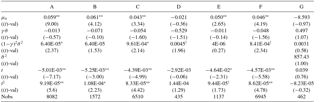
informative.Table 4displays ordinary least square (OLS)
esti-mates for the first moments, that is, the first two equations of
system (17). The regressions in columns D and G, complete
spells with an increasing surplus (τ ≥0) and, respectively,
job movers, are badly identified due to a low number of obser-vations. The other columns reveal some common patterns. First, the intercept and the experience profile are virtually the same in all regressions. Second, the coefficient ofγ σis negative, though never statistically significant, while it is expected to be positive. This term captures the earlier result from the tenure distribution
analysis that the drift in the surplust depends positively on
experience at job startS, equivalent to stating that jobs starting at later age last longer. Given thatγ >0, the model predicts that workers are able to capture part of the surplus increase, and hence, that the tenure profile in jobs starting at higher ages should be steeper. The data reject this implication.
Table 5presents linear regression results for the second mo-ments, that is, the last three equations of system (17). The es-timates invoke three observations. First, contrary to the pre-dictions of our model, the estimates for (γ σ)2 are negative.
The model predicts a hump shape in the variance ofwt over
the course of a job spell, with low variances in the beginning
Table 4. OLS estimates first moments (first two equations) of system (17)
A B C D E F G
μ0 0.059∗∗ 0.061∗∗ 0.043∗∗ −0.021 0.050∗∗ 0.046∗∗ −8.593
((t)-val) (9.00) (4.12) (3.34) (−0.36) (2.65) (4.19) (−0.97)
γσ¯ −0.013 −0.071 −0.054 −0.529 −0.011 −0.048 0.497
((t)-val) (−0.57) (−0.10) (−1.60) (−1.51) (−0.14) (−1.56) (1.07) (1−γ)2σ¯2 6.40E-05∗ 6.40E-05 9.61E-04∗ 0.0045† 4E-06 8.41E-04† 0.0031
((t)-val) (2.37) (1.53) (2.14) (1.96) (0.27) (2.34) (0.58)
¯
σ2 857.43
((t)-val) (1.00)
t −5.01E-03∗∗ −5.25E-03∗∗ −4.39E-03∗∗ −2.92E-03 −4.64E-02∗ −4.57E-03∗∗ 0.039
((t)-val) (−7.17) (−3.00) (−4.99) (−0.06) (−2.31) (−5.58) (0.76)
t2 9.19E-05∗∗ 1.08E-04∗ 8.33E-05∗∗ 1.44E-04 9.44E-05† 8.62E-05∗∗ −8.23E-05
((t)-val) (5.6) (2.23) (4.42) (1.29) (1.73) (4.78) (−0.32)
Nobs 8082 1572 6510 435 1137 6945 462
NOTES: Significance levels:†: 10%;∗: 5%;∗∗: 1%. Statisticalt-values in parentheses under estimated coefficients.
Columns A to F correspond to the first moment equations for job stayers (first equation of system (17)), where A: all stayers, B: completed spells, C: incomplete spells, D: completed positive surplus change spells, E: completed negative surplus change, F: incomplete plus completed positive surplus change; Column G corresponds to the first moment equation for job movers (second equation of system (17)).
We allow for a concave experience (t,t2) profile in each estimated equation.
and the end of a job. The data tell the opposite. Thus, while the model accurately captures the concavity in the tenure profile
in the first moment ofwt, in particular when accounting for
downward rigidity in wages, it does not capture the pattern in its
second moment. Second, the varianceσ2
z +σu2 is a factor four
times higher for job movers than for job stayers. This suggests that the labor market is not a Walrasian market with a continuum of outside offers available at any time, where workers who want to change jobs can just pick the best option out of this contin-uum. Outside offers come along randomly, so that there are large jumps in the wage profile at the moment of job change. Third, within the group of job stayers, the variance does not seem to be constant across subgroups either; it is the largest for the in-complete spells and the smallest for the in-complete spells with a declining surplus (τ <0), whereas the complete spells with
an increasing surplus fall somewhere in between. The low vari-ance for complete spells with a declining surplus fits the notion of downward wage rigidity. When wages are rigid, one would not expect a whole lot of variance.
Table 6presents formal Wald tests for the above hypothe-ses, reportingχ2 statistics and associatedp-values for tests of
equality of estimates across nested model specifications for the system (17). All tests start from the full model (using the whole
number of observations, on both stayers and movers), except for horizontal panel 6 that presents nested hypotheses tests for the subsample of job stayers. Panel 1 presents three Wald tests for the null hypotheses{γs=γm},{σ2s =σ
2
m}, and the joint null
{γs =γmandσ2s =σ
2
m}, wheresindexes stayers andmmovers.
The null{γs =γm}cannot be rejected, but the null{σ2s =σ
2
m}
can. Hence, the joint null {γs=γm andσ2s =σ
2
m}is also
re-jected. This suggests that there is excess wage variance for job movers. Hence, our assumption of a Walrasian market for out-side job offers is not respected in the data. Panel 2 presents a Wald test for{γneg=γrest}, whereγnegis estimated only for the
completed job spells with a negative surplus change,τ <0,
whileγrestis estimated on the rest of the sample. We fail to reject
the null ofγ being the same for the negative job spells and for the rest of the observations.
Panel 3 presents the Wald test of {γdrift=γnondrift}, where
γdriftis estimated from the drift term in the first-moment
equa-tions, whileγnondriftis estimated from all other instances where
it appears in the system (17). As expected from earlier remarks, we strongly reject this null. Panel 4 presents the Wald test of
{γfirst=γsecond}. This restriction cannot be rejected. Panel 5
displays the result of the Wald for{σ2
z,s =σz,m2 }, that is,
test-ing for equality of the variance of the permanent shocks,σ2
z,
Table 5. OLS estimates second moments (last three equations) of system (17)
A B C D E F G H I
(1−γ)2σ¯2
−0.0081∗∗ −0.010† −0.025∗∗ −0.016 −0.010∗ −0.019∗∗ −0.089
((t)-val) (−3.28) (−1.88) (−4.55) (−1.16) (−1.82) (−4.42) (−0.53)
σz2+2σu2 0.027∗∗ 0.025∗∗ 0.042∗∗ 0.032∗∗ 0.025∗∗ 0.036∗∗ 0.156∗∗
((t)-val) (12.28) (8.33) (8.49) (3.51) (7.73) (9.60) (2.98)
σu2 0.0042∗∗ 0.0043∗∗
((t)-val) (14.01) (13.28)
Nobs 8082 1572 6510 435 1137 6945 462 5789 4972
NOTES: Significance levels:†: 10%;∗: 5%;∗∗: 1%. Statisticalt-values in parentheses under estimated coefficients.
Columns A to F correspond to the second moment for job stayers (third equation of system (17)), where A: all stayers, B: completed spells, C: incomplete spells, D: completed positive surplus change spells, E: completed negative surplus change, F: incomplete plus completed positive surplus change; Column G corresponds to the second moment for job movers (fourth equation of system (17)); Columns H to I correspond to the covariance moment (last equation of system (17)), with H using all stayers and I using the incomplete plus positive completed surplus change spells.
We use the residuals computed from corresponding first moments of system (17), upgraded with concave experience profiles, as dependent variables in all second-moment equations.
Table 6. Nested hypotheses tests for subset estimates system (17)
1:γs =γm, ¯σs2=σ¯m2
Waldγs=γm χ2=0.37 (Prob> χ2=0.54)
Wald ¯σs2=σ¯m2 χ2=5.60∗(Prob> χ2=0.018)
Joint Waldγs=γmand ¯σs2=σ¯m2 χ2=5.80†(Prob> χ2=0.055)
2:γneg=γrest
Waldγneg=γrest χ2=1.64 (Prob> χ2=0.20)
3:γdrift=γnondrift
Waldγdrift=γnondrift χ2=31.43∗∗(Prob> χ2<0.0001)
4:γfirst=γsecond
Waldγfirst=γsecond χ2=0.45 (Prob> χ2=0.50)
5:σz,s2=σz,m2
Waldσz,s2=σz,m2 χ2=37.45∗∗(Prob> χ2<0.0001)
6:σz,s,inc2=σz,s,neg2,σz,s,inc2=σz,s,pos2,σz,s,neg2=σz,s,pos2
Waldσz,s,inc2=σz,s,neg2 χ2=2.08 (Prob> χ2=0.149)
Waldσz,s,inc2=σz,s,pos2 χ2=0.04 (Prob> χ2=0.833)
Waldσz,s,neg2=σz,s,pos2 χ2=1.82 (Prob> χ2=0.177)
Joint Waldσz,s,inc2=σz,s,neg2andσz,s,inc2=σz,s,pos2 χ2=2.17 (Prob> χ2=0.338)
NOTES: Significance levels:†: 10%;∗: 5%;∗∗: 1%. Statisticalp-values in parentheses.
Detailed description for each hypothesis test can be found in the text; “m” indexes movers, “s” stayers, “inc” incomplete job spells, “pos” (“neg”) completed positive (negative) surplus change job spells. The test in panel 4 is de facto implemented asH0:k21=k2, wherek1=1−γfirstandk2=(1−γsecond)2, since, ask2is estimated negative in the corresponding linear
regression,γsecondcannot take a real value in that particular specification.
All specifications allow for concave experience (t,t2) profiles.
across movers and stayers. This null is clearly rejected. Given our result from panel 5, we now start from a model where
we allow for different σ2
z,s and σz,m2 : in panel 6 we test in
subsamples of job stayers only the following null hypotheses: {σz,s,2 inc=σz,s,2 neg},{σz,s,2 pos=σz,s,2 neg},{σz,s,2 inc=σz,s,2 pos}, and, respectively, the joint {σ2
z,s,inc=σz,s,2 neg andσz,s,2 inc=σz,s,2 pos},
where inc indexes incomplete job spells, neg completed job
spells withτ<0, as above, and pos completed job spells
withτ ≥0. These tests show that once we account for the
differences inσz2between movers and stayers, there are no fur-ther statistical differences between the estimates for subsamples of stayers: indeed, we cannot reject any of the null hypotheses from panel 6 ofTable 6.
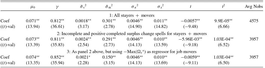
Once we allow movers and stayers to possibly have different
wage variances, the new FGNLS estimates reported inTable 7
show that movers have indeed a much higher wage variance at job separation; our favorite specification in panel 3 suggests
σm≃8.4σs. In this case, γ is estimated in a much narrower
range, between 0.81 and 0.85, with all the other parameter
esti-mates close to the values fromTable 3. We repeat the previous
calculation of the return to tenure, this time withσs =0.04, and γ =0.8. We obtain a return that is exactly the same as computed before,σsπ =0.04×0.14=0.56%, again mostly due to the
fall in the outside option. The drift inptaccounts now for only γ σsπ =(1−0.8)×0.56%=0.11%. Hence, once we adjust
our empirical model to allow for downward rigidity of wages and for the non-Walrasian market for job switches, about 80% of the wage returns to tenure is due to selectivity on the outside wages.
APPENDIX: CONDITIONAL EXPECTATION AND VARIANCE OFτ
A.1. Completed Spells
For the subsequent derivations, it is useful to add the
pa-rameter for initial surplus,, as an argument to the survival
function of job tenures in Equations (8) and (9), thusF(τ, )
andf(τ, ). Leth(ω, τ, , ) be the density ofτ=ωfor
0< τ < conditional on A(). Comparing this density to
Table 7. FGNLS estimates system (17), with different wage variances for stayers and movers
μ0 γ σ¯s2 σ¯m2 σu2 σz2 t t2 Avg Nobs
1: All stayers + movers
Coef 0.071∗∗ 0.812∗∗ 0.0018∗∗ 0.301∗∗ 0.0046∗∗ 0.011∗∗ −0.0057∗∗ 9.9E-05∗∗ 4575
((t)-val) (13.94) (36.61) (3.17) (2.78) (14.90) (14.82) (−9.48) (6.66) 2: Incomplete and positive completed surplus change spells for stayers + movers
Coef 0.073∗∗ 0.811∗∗ 0.0024∗∗ 0.291∗∗ 0.0046∗∗ 0.010∗∗ −5.96E-03∗∗ 1.03E-04∗∗ 3957
((t)-val) (13.39) (35.83) (2.54) (2.73) (14.13) (13.59) (−9.18) (6.52) 3: As panel 2 above, but using−Max(τ∗) as regressor for job movers
Coef 0.074∗∗ 0.852∗∗ 0.0021∗ 0.150∗∗ 0.0046∗∗ 0.010∗∗ −0.0059∗∗ 1.03E-04∗∗ 3957
((t)-val) (13.35) (35.94) (2.28) (3.15) (14.13) (13.69) (−9.11) (6.50)
NOTES: Significance levels:∗: 5%;∗∗: 1%. Statisticalt-values in parentheses under estimated coefficients. We allow for a concave experience (t,t2) profile in all equations of system (17).
g(ω, τ), there is one additional condition: =0. Hence,
Substitution of Equation (7) in the above yields
h(ω, τ, , )= ω
For the calculation of the second moment of a first differential ofτ, E[2τ|A()], we apply the joint density ofτ−1=ω
andτ=ω+χ, for 1≤τ ≤/, conditional onA():
h(ω+χ ,1, −τ +1, ω)·h(ω, τ −1, , ).
The second moment ofτis thus given by
E
We use numerical integration for the evaluation of the integral above. The variance is subsequently derived by the standard ex-pression var[τ|A()]=E[2τ|A()]−E[τ|A()]2.
A.2. Incomplete Spells
Leth∗(ω, τ, , ) be the density ofτ=ωconditional on
B(). Application of the Bayes’ rule yields
h∗(ω, τ, , )= ∞F(−τ, ω)g(ω, τ)
is evaluated numerically, since it does not have an analytical solution.
The variance ofτ =τ−τ−1, for 1≤τ ≤,
condi-tional onB() is then derived from the first and second
mo-ments ofτ, analogous to the completed spells case discussed
above.
ACKNOWLEDGMENTS
The authors thank the editors Keisuke Hirano and Shakeeb Khan, an anonymous associate editor, two anonymous refer-ees, Rob Alessie, Gadi Barlevi, Richard Blundell, Jeff Camp-bell, Bas van der Klaauw, Jim Heckman, Dale Mortensen, Derek Neal, Randall Olsen, Aureo de Paula, Miguel Portela, Jean Marc Robin, Rob Shimer, Chris Taber, Aico van Vu-uren, Robert Waldmann, and audiences in a large number of seminars and conferences. The authors also acknowledge Nick Williams and Lennart Janssens for assistance in handling the data. The usual disclaimers apply. An online folder contain-ing a web appendix with supplementary details on the esti-mations, the data, and our estimation programs is accessible atwww.sebastianbuhai.com/tenureprofiles. Buhai gratefully ac-knowledges partial funding for this project through Marie Curie IOF grant PIOF-GA-2009-255597, awarded by the European Commission.
[Received October 2011. Revised April 2013.]
REFERENCES
Abowd, J. M., and Card, D. (1989), “On the Covariance of Earnings and Hours Changes,”Econometrica, 57, 411–445. [245,248]
Abowd, J. M., Kramarz, F., and Margolis, D. (1999), “High Wage Workers and High Wage Firms,”Econometrica, 67, 251–333. [245]
Abraham, K. G., and Farber, H. S. (1987), “Job Duration, Seniority, and Earn-ings,”American Economic Review, 7, 278–297. [245]
Altonji, J. G., and Shakotko, R. A. (1987), “Do Wages Rise With Seniority?,” Review of Economic Studies, 54, 437–459. [245]
Altonji, J. G., and Williams, N. (1997), “Do Wages Rise With Job Seniority? A Reassessment,” NBER Working Paper No. 6010, National Bureau of Economic Research. [245]
——— (1999), “The Effects of Labor Market Experience, Job Seniority and Job Mobility on Wage Growth,” inResearch in Labor Economics, (Vol. 17), ed. S. Horwitz, Greenwich, CT: JAI Press. [252]
——— (2005), “Do Wages Rise With Job Seniority? A Reassessment,” Indus-trial and Labor Relations Review, 58, 370–397. [245]
Beaudry, P., and DiNardo, J. (1991), “The Effect of Implicit Contracts on the Movement of Wages Over the Business Cycle: Evidence From Micro Data,” Journal of Political Economy, 99, 665–688. [246]
Browning, M., Ejrnaes, M., and Alvarez, J. (2010), “Modeling Income Processes With Lots of Heterogeneity,”Review of Economic Studies, 77, 1353–1381. [253]
Buchinsky, M., Fougere, D., Kramarz, F., and Tchernis, R. (2010), “Interfirm Mobility, Wages, and the Returns to Seniority and Experience in the US,” Review of Economic Studies, 77, 972–1001. [245]
Burdett, K., and Mortensen, D. T. (1998), “Wage Differentials, Employer Size, and Unemployment,”International Economic Review, 39, 257–273. [246] Dixit, A. K. (1989), “Entry and Exit Decisions Under Uncertainty,”Journal of
Political Economy, 97, 620–638. [245]
Dixit, A. K., and Pindyck, R. S. (1994),Investment Under Uncertainty, Prince-ton, NJ: Princeton University Press. [245,246,247]
Dustmann, C., and Meghir, C. (2005), “Wages, Experience and Seniority,” Review of Economic Studies, 72, 77–108. [245]
Farber, H. S. (1994), “The Analysis of Interfirm Mobility,”Journal of Labor Economics, 12, 554–593. [248,251]
——— (1999), “Mobility and Strategy: The Dynamics of Job Change in Labor Markets,” inHandbook of Labour Economics(Vol. 3-B), eds. O. Ashenfelter and D. Card, Amsterdam: North-Holland. [245]
Feller, W. (1968),An Introduction to Probability Theory and its Applications (Wiley Series in Probability and Mathematical Statistics, Vol. 2), New York: Wiley. [247]
Horowitz, J. L., and Lee, S. (2002), “Semiparametric Estimation of a Panel Data Proportional Hazards Model With Fixed Effects,” Chapter 3, unpublished Ph.D. dissertation, University of Iowa. [248]
Jacobson, L. S., LaLonde, R. J., and Sullivan, D. G. (1993), “Earnings Losses of Displaced Workers,”American Economic Review, 84, 685–709. [249]