11 (2001) 1 – 15
The option on
n
assets with exchange rate and
exercise price risk
Spiros H. Martzoukos *
Department of Public and Business Administration,Uni6ersity of Cyprus,75Kallipoleos Str., P.O.Box20537,CY1678Nicosia,Cyprus
Received 19 February 1999; accepted 15 October 1999
Abstract
Solutions to the call option on the maximum or the minimum ofn assets are explicitly provided when the exercise price is stochastic, and all assets carry both asset price and exchange rate risk in an+1 country model with 2(n+1) state variables. The model can be seen as an extension of Johnson (Johnson, H., 1987. Options on the maximum or the minimum of several assets. Journal of Financial and Quantitative Analysis 22, 227 – 283), Margrabe (Margrabe, W., 1978. The value of an option to exchange one asset for another. Journal of Finance 33, 177 – 186), and Reiner (Reiner, E., 1992. Quanto mechanics, RISK, March, 59 – 63), and it is useful for valuation of both financial and real options. As an application, a contract is valued that allows a portfolio manager to participate in the out-performance of the returns of international assets, portfolios or stock indexes. © 2001 Elsevier Science B.V. All rights reserved.
JEL classification:G12; G13
Keywords:Derivatives models; Exchange rate risk; Measure transform; Real options
www.elsevier.com/locate/econbase
1. Introduction
Valuation models for options with one underlying risky asset and a stochastic exercise price have already appeared in the literature. They include the European option of Margrabe (1978) to exchange one asset for another, the European option
* Tel.: +357-2-892289; fax: +357-2-339063.
E-mail address:[email protected] (S.H. Martzoukos).
of Fischer (1978) when the exercise price is uncertain, the investment model of McDonald and Siegel (1985) with a shutdown option, the model of McDonald and Siegel (1986) of the value of waiting to invest, the option of Myers and Majd (1990) to abandon an existing investment for its salvage value, and the empirical testing of Quigg (1993) of the option to wait to develop vacant land.
Contingent-claim models on n underlying risky assets also exist in the financial economics literature. The valuation methodology usually requires a high degree of computational intensity, but the constant increase in computational power available to financial researchers has considerably enhanced the attractiveness of such models. Such work includes Broadie and Detemple (1997), Barraquand and Mar-tineau (1995), Boyle and Tse (1990), Boyle et al. (1989), Johnson (1987), and Kamrad and Ritchken (1991). These contributions provide a general valuation methodology, numerical or analytic, and their applicability is not limited to traded options alone, an area that during the last decade has shown a tremendous proliferation in both exchange-traded and over-the-counter instruments. Instead, they are directly extendible to decision making and valuation of real investments under uncertainty and irreversibility — see Pindyck (1991), Dixit and Pindyck (1994), or Trigeorgis (1996) — the area usually referred to as real options. These results allow the treatment of real options with multiple, mutually-exclusive invest-ment alternatives.
Contingent claim valuation with exchange rate risk is established in Garman and Kohlhagen (1983), and Grabbe (1983). They value options on foreign currency and demonstrate that the risk-neutral drift of the underlying asset equals the home riskless rate of interest minus the foreign riskless rate of interest. The foreign rate of interest can be interpreted as a dividend yield that the option holder would capture only if a call option is exercised. Real options applications with exchange rate risk appear in Mello et al. (1995). They consider a multinational firm that can shift production back and forth between the home and a foreign country. They use a partial irreversibility model as opposed to the complete irreversibility that is implied by the real options in the context of the applications. Applications in financial options have appeared in Reiner (1992), Jamshidian (1993), and Kat and Roozen (1994) where options on foreign stocks are valued when the exchange rate relevant to option exercise is predetermined (the ‘quanto’ models).
In the case of multivariate contingent-claim models on the best of n underlying assets, the usual assumption is that the exercise price is constant. Overall, this is a somewhat restrictive assumption. In this paper the valuation methodology of options onnunderlying assets is extended when the exercise price is stochastic, and there is exchange rate risk present for all assets in an+1 country model. In effect, the case of 2(n+1) state variables that follow correlated Brownian motion pro-cesses are treated. Some of the applications provided nest the models known as quantos as special cases. The results can be applied for valuation of both financial and real (investment) options. The implementation for the European option on n
For clarity of presentation, the extension to Johnson’s model for a stochastic exercise price in the absence of exchange rate risk is first provided. Then the model is extended when all assets (including the exercise price) are in foreign countries but the exchange rates relevant to option exercise are predetermined in the quanto context; and then when all assets are in foreign countries without any exchange rate protection. These results extend a previous work (Martzoukos, 1994, 1995). They are demonstrated (with both the analytic and a multivariate lattice technique) in the valuation of a contract that gives a portfolio manager the option to exchange the proceeds from a foreign (index) investment for the best of other foreign (index) investments.
2. Derivation of the n-dimensional model
There are n+1 risky asset prices. These are the prices of the option’s n
underlying assets, and the stochastic exercise price. Each follows geometric Brown-ian motion of the form
dS
S=(mS−dS)dt+sSdzS, (1a)
where the dz terms denote the increment of standard Wiener processes with instantaneous correlation coefficients r. Each asset pays a continuous payoff dS.
The drift mS−dS and volatility sS terms can be either constant or deterministic
functions of time, and standard regularity conditions are assumed to hold. The dividend yields may represent actual cash flow, as in the case of stock options, or may be equivalent to one, like in the case of foreign exchange. McDonald and Siegel (1985, 1986) provide real options applications where the dividend yields represent the difference between the equilibrium total expected rate of return and the actual expected growth rate on the underlying assets, as shown by McDonald and Siegel (1984) drawing on Constantinides (1978). Brennan (1991) provides a convenience yield interpretation for the dividend yield. In general, a continuous time capital asset pricing model like in Merton (1973a) or Breeden (1979) is assumed to hold. Under the risk-neutral measure total required returns equal the riskless rate of interest r, and the assets’ law of motion
dS
S=(r−dS)dt+sSdzS. (1b)
The price Pof a multivariate contingent claim on several assets is described (see for example, Cox et al., 1985) by a partial differential equation (PDE) of the form
(P/(t=rP−%
I%
[(r−dI%)I% (P/(I%]
−0.5
!
%I% [sI%
2I%2(2P/(I%2]+ %
I%,J%,I%"J%
[sI%,J%I%J% (
where I% and J% denote all pairs of the stochastic variables, with instantaneous
covariance sI%,J%. Summation is always over all stochastic assets. When the exercise
price X is similarly stochastic, the explicit dependence is shown by rewriting PDE (2) as
where asset X pays a constant dividend yielddX.
To remove the dependence on the stochastic variable X, one must reduce the dimensionality of the contingent claim with n+1 stochastic variables to one withn
stochastic variables. To achieve this a change of variables is employed from all pairs of I% and J% to I=I%/X and J=J%/X, where the exercise price X is used as a
numeraire. PDE (3) that follows gives the solution (see Appendix A for the proof) with the variable f defined as P/X
(f/(t=dXf−%
Note the similarity of the derived PDE in (3) with (2). Two features are notable. First, the variance of the underlying assets and the covariances are adjusted to account for the uncertain exercise price used as a numeraire. Second, the riskless rate of interest, r, does not appear in the model, and is replaced by the dividend yield on the exercise price,dX. These results are sufficient to allow contingent claims
models on the best of n assets to be extended to the case of a stochastic exercise price. Simply replace the riskless rate with dX, all variances sI2% with sI2, and all
covariances sI%,J% withsI,J.
2.1. The european call option with stochastic exercise price
The solution to the European call option on the maximum or minimum (max/
exp(−rT)
&&&
n+1
F[max/min(S1,S2, . . .,Sn)−X]
+d
S1dS2. . . dSndX
discounted at the riskless rate of interest, where T is the option’s maturity. The results are extended in Johnson (1987), finding that the price of a European call option on the maximum cmaxis a function of the asset prices S1, . . .,Sn,X, time to
maturity T, the dividend yields dI%, dX, and the instantaneous variances and
covariances of the transformed assets. Its price equals
cmax=S1exp(−dS1T)
where I% and J% represent all pairs of the n assets, and Iand J their transformed
counterparts.
2 , etc. are defined as in Eq. (6a), and the tripled indexed correlation
coefficients (like in Johnson) are
rIIJ=(sI−rI,JsJ)/sI,J, (6g)
rIJK=(sI
2
−rI,JsIsJ−rI,KsIsK+rJ,KsJsK)/(sI,JsI,K). (6h)
cmin=S1exp(−dS1T)
where again Eqs. (6a), (6b), (6c), (6d), (6e), (6f), (6g) and (6h) hold. For numerical solutions to the cumulative multivariate normal Nn(. . .) see the references in Johnson (1987) and in Boyle and Tse (1990).
The American option on the maximum or the minimum of n assets can be handled like in Boyle et al. (1989), and Kamrad and Ritchken (1991). One only needs to replace the riskless rate of interest, r, with the dividend yield on the exercise price, dX, and use equations (Eqs. (6a), (6b) and (6c)) to adjust the asset
variances and correlations. Barraquand and Martineau (1995) give simulation methods for both European and American-type multivariate claims that can be similarly extended for a stochastic exercise price.
3. The model with exchange rate risk
Reiner (1992), Jamshidian (1993) and Kat and Roozen (1994) value ‘quantos’, contracts that involve both foreign exchange and stock price risk. Note that quanto refers to the case where the option payoff is in home currency, so the option is effectively protected against foreign exchange risk. As also discussed in Hull (1997) (pp. 298 – 301), the risk-neutral drift of a foreign stock (quanto), if viewed from the perspective of the home country, equals the foreign risk-neutral drift minus the covariance between the underlying asset and the exchange rate, a result called ‘Siegel’s paradox’. In all the relations that follow, the home country’s exchange rate convention is considered, where home is the country of the option holder. The sign of the correlation between the exchange rate and the foreign asset would be reversed if the foreign convention was used to define exchange rates.
quanto’, that offers the right to exchange one foreign asset for the best of other foreign assets, and offers protection against exchange rate risk. Second the option to exchange a foreign asset for the best of other foreign assets was priced, but without the exchange rate protection. In the following relations, SI% denotes the n
foreign assets, with SI%,SJ% each pairwise combination, and SXdenotes a foreign
asset that serves as the exercise price. Similarly, EI%, EJ%, and EX denote the
exchange rates, and all state variables follow correlated geometric Brownian motion processes.
One first prices the exchange quanto. Again one needs to solve PDE (3). All
foreign assets SI% (and likewise the one used as an exercise price) follow from the
perspective the risk-neutral process
dSI%
SI% =(rI−dSI%−sSI%,sEI%rSI%,EI%) dt+sSI%dzSI%,
where the rate rI denotes the foreign riskless rate for country I, dSI% denotes the dividend yield on the foreign asset from the perspective of the foreign country, and
sSI% the instantaneous S.D. of the foreign asset in the respective foreign currency. One can now value the exchange quanto option given that the dividend yields of the underlying assets dI%, and of the exercise price dX are known from the author’s
perspective
dI%=r−rI+dSI%+sSI%sEI%rSI%,EI%, (8a)
dX=r−rX+dSX+sSXsEXrSX,EX (8b)
withsEI%, andrSI%,EI%the instantaneous S.D. of the exchange rate, and the instanta-neous correlation between the foreign asset and the exchange rate. This correlation is only needed to evaluate each dividend yield. The S.D.s of the underlying assets
sI%, and of the exercise price sX, and their correlationsrI%,J%, rI%,Xare still needed in
order to use the call option on the maximum or the minimum that were derived earlier. These are simply
sI%=sSI%, sX=sSX, (8c)
rI%,J%=rSI%,SJ%, rI%,X=rSI%,SX, (8d)
Eqs. (8a), (8b), (8c) and (8d) provide the dividend yields, standard deviations and correlations of the n normalized foreign (quanto) assets. They allow, together with Eqs. (5), (6a), (6b), (6c), (6d), (6e), (6f), (6g), (6h) and (7), pricing of the call option on the maximum or minimum of n foreign assets in exchange for another foreign asset. All foreign assets are protected against exchange rates’ movements (in the quanto context), since each is translated in home currency using a predetermined (fixed) exchange rate.
Second the exchange option will be demonstrated without such exchange rate
protection. Each underlying asset and the exercise price are the product of a foreign asset SI%with the relevant exchange rateEI%. Each foreign asset (before translation
perspec-tive of the home country (as discussed earlier in the quanto context). The foreign currency from the home country perspective has a risk-neutral drift ofr−rI. Using Ito’s lemma it was found that under risk-neutrality all underlying (foreign) assetsI%,
and similarly the exercise priceX, follow (from the author’s perspective) the law of motion
dI%
I% =(r−dSI%) dt+sI%dzI%.
Thus, the dividend yields dI%,dXneeded in the option model are simply
dI%=dSI%, and dX=dSX, (9)
The instantaneous S.D. of each underlying foreign asset, and of the exercise price
X equal
sI%=(sSI%
2
+sEI%
2
+2sSI%sEI%rSI%,EI%), (10a)
sX=(sSX
2
+sEX
2
+2sSXsEXrSX,EX). (10b)
Again and in order to solve the problem one starts from PDE (2) and work the way to PDE (3). To use Eq. (2) one needs to get the covariance among all foreign assets sI%J%, and between the foreign assets and the exercise price sI%X, as functions
of the S.D.s sSI%, sSJ%, sSX, sEI%, sEJ%, and sEX, and the correlations between the
foreign assets and the exchange rates rSI%,EI%, . . ., rSI%,SJ%, . . ., rEI%,EJ%, . . . With the
use of standard stochastic calculus one gets
sI%,J%=(sSI%sSJ%rSI%,SJ%+sSI%sEJ%rSI%,EJ%+sEI%sSJ%rEI%,SJ%+sEI%sEJ%rEI’,EJ%), (11a)
and
sI%,X=(sSI%sSXrSI%,SX+sSI’sEX%rSI%,EX+sEI%sSXrEI%,SX+sEI%sEXrEI%,EX). (11b)
PDE (3) with the usual boundary conditions again defines the solution for the price of American or European options on nassets with a stochastic exercise price
X (when all foreign assets are affected by exchange rate risk). The dividend yields, the S.D.s, and the covariances/correlations are given from Eqs. (9), (10a), (10b), (11a) and (11b). These equations, together with Eqs. (5), (6a), (6b), (6c), (6d), (6e), (6f), (6g), (6h) and (7) define the European call option on the maximum and the minimum in exchange for foreign asset X. Similarly, finite difference methods, multinomial lattice, or Monte Carlo simulations can also be used with the use of Eqs. (9), (10a), (10b), (11a) and (11b).
4. An application in international portfolio management
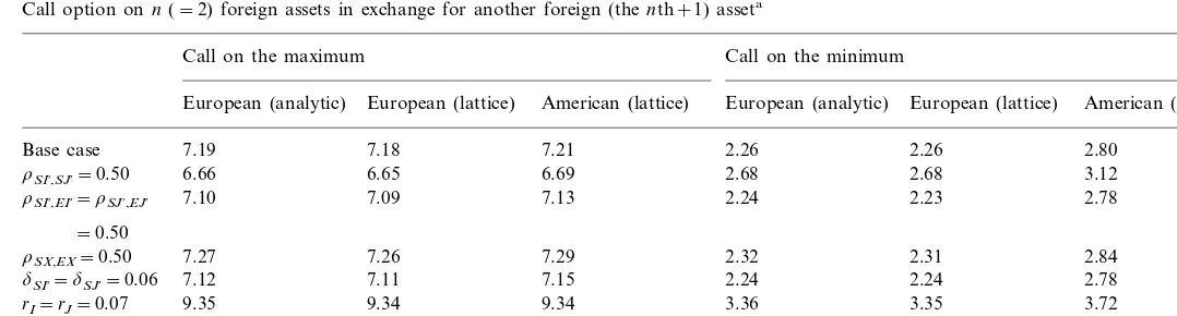
thereby wishing the option to give it up for assets in country I, or J; or simply wishing an option on the outperformance between the best of (assets) ofIorJ, and those of countryX. A call option on the maximum is obviously more valuable than a call option on the minimum. This option can either be of the quanto type for all three assets, or they are all unprotected against exchange rate risk (and of course it is straightforward to modify the results for the case where some assets are protected and some are not). The first contract type will offer participation in the outperfor-mance of the assets in the respective foreign countries regardless of the movements of the exchange rates; the second’s performance will in addition depend on exchange rate risk and is expected to be more valuable (and more costly). The numerical results for the call the option on the maximum and on the minimum appear in Table 1 for the quanto contract, and Table 2 for the unprotected contract. In both tables computations are presented using the analytic results (1st and 4th columns for a European option), and a 200-steps 2-dimensional lattice framework (for both the European and the American options). The comparison between the analytic and the (European) lattice confirms the accuracy of the lattice implementation. For the base case it was assumed that all foreign assets pay dividend yields of 3%, all riskless rates are 5%, all instantaneous standard devia-tions are 10%, and all correladevia-tions are 25%. All underlying assets (as well as the asset serving as the exercise price) are currently priced at 100 in the respective currencies, with the exchange rates for the quanto contract fixed to the ones prevailing at time zero (which for simplicity are assumed to equal unity). Thus, any differences between the two contract types depend on the option dynamics alone. From the earlier analysis in Stulz (1982) and Johnson (1987) the impact of an increase in the riskless rate (of the home country) or the dividend yields of the underlying assets is known. An increase in the riskless rate, would increase the option value for both the call on the minimum and the call on the maximum; and an increase in dividend yields of the underlying assets would effectively decrease their value and the value of call option prices. In this case the dynamics are more complex. When the contract is not of the quanto type, the riskless rates of all four countries (home and the three foreign) do not appear in the model and subse-quently do not affect valuation. The riskless rate has been replaced by the dividend yield of the asset serving as an exercise price, so an increase of that yield will also increase the value of the options on the maximum and the option on the minimum (see last line of Table 2). When the contract is of the quanto type, the riskless rate is replaced by the effecti6e dividend yield of the exercise price as in Eqs. (8a) and
S
Call option onn(=2) foreign assets in exchange for another foreign (thenth+1) asseta
Call on the minimum Call on the maximum
American (lattice) European (analytic) European (lattice) American (lattice) European (analytic) European (lattice)
2.26 2.26 2.80
aAll with exchange rate protection (Quanto type). For the base case, the underlying foreign assetsSI%,SJ%, and the exercise priceSX, all equal 100 (in the respective foreign currency units), the applicable exchange ratesEI%,EJ%, andEXarefixed(quanto contract) to unity (for simplicity of exposition), the local riskless interest raterand the foreign riskless ratesrI,rJ, andrXall equal 0.05, the time to maturity of the option is 1 year, the dividend yields of the
assets in the respective countriesdSI%,dSJ%, anddSXequal 0.03, all S.D.s of the foreign assets and the exchange ratessSI%,sEI%,sSJ%,sEJ%,sSX, andsEX, equal
0.10, and all correlationsrSI%,EI%,rSI%,EJ%,rSI%,EX,rSJ%,EI%,rSJ%,EJ%,rSJ%,EX,rSX,EI%,rSX,EJ%,rSX,EX,rSJ%,SX,rSI%,SJ%,rSI%,SX,rEJ%,EX,rEI%,EJ%,rEI%,EX, equal 0.25.
H
.
Martzoukos
/
J
.
of
Multi
.
Fin
.
Manag
.
11
(2001)
1
–
15
11
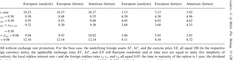
Call option onn(=2) foreign assets in exchange for another foreign (nth+1) asset
Call on the maximum Call on the minimum
European (lattice)
European (analytic) European (lattice) American (lattice) European (analytic) American (lattice)
3.92
3.15 3.15
10.27 Base case 10.25 10.23
8.50 8.48 8.55 4.50 4.96
rSI%,SJ%=0.50 4.50
4.05 4.05 4.62
8.95
rEI%,EJ%=0.50 8.93 9.00
3.68 4.33
3.68 9.38
9.30 rSI%,EJ%=rSJ%,EJ% 9.32
=0.50
9.94 9.93 10.02 3.05 3.85
dSI%=dSJ%=0.06 3.06
4.10
12.16 12.14 12.14 4.11 4.72
dSX=0.06
aAll without exchange rate protection. For the base case, the underlying foreign assetsSI%,SJ%, and the exercise priceSX, all equal 100 (in the respective foreign currency units), the applicable exchange rates EI%, EJ%, and EXwill fluctuate randomly and at time zero are equal to unity (for simplicity of exposition), the local riskless interest raterand the foreign riskless ratesrI,rJ, andrXall equal 0.05, the time to maturity of the option is 1 year, the dividend
yields of the assets in the respective countriesdSI%,dSJ%, anddSXequal 0.03, all S.D.s of the foreign assets and the exchange ratessSI%,sEI%,sSJ%,sEJ%,sSX,
andsEX, equal 0.10, and all correlationsrSI%,EI%,rSI%,EJ%,rSI%,EX,rSJ%,EI%,rSJ%,EJ%,rSJ%,EX,rSX,EI%,rSX,EJ%,rSX,EX,rSJ%,SX,rSI%,SJ%,rSI%,SX,rEJ%,EX,rEI%,EJ%,rEI%,EX,
effecti6edividend yields in those countries and would increase the quanto protected
option values (3rd line from the bottom, Table 1). An increase in the dividend yields of any of the assets in countries I or J would decrease all option values in both the quanto and the unprotected contracts (5th line, Table 1, and 2nd from the bottom, Table 2). Also, the quanto contracts are affected by the correlation between a foreign asset value and the exchange rate of that country (seen from the author’s perspective). An increase in that correlation increases theeffecti6edividend
yield of the assets in the respective country. In the case of the underlying assets such an increase results in a decrease in option values (3rd line, Table 1); and in the case of the asset in country Xresults in an increase in option values (4th line, Table 1). The correlations among several variables can affect option values significantly. In the absence of exercise price and exchange rate risk, a higher correlation between the two underlying assets will increase the value of the option on the minimum, and will decrease the value of the option on the maximum. In this case the dynamics are again more complex. For the case of the quanto option, the correlation among the underlying (foreign) assets will increase the effecti6e correlation in Eq. (4b), or
equivalently Eq. (6c). Subsequently, the option values on the minimum increase, and the option values on the maximum decrease (2nd line, Table 1). For the case of the unprotected exchange option, Eqs. (4b) and (6c) are affected through Eq. (11a). The effecti6ecorrelation between the asset in country I and that in country J increases with an increase in correlations between the two underlying foreign assets (2nd line, Table 2). Also between the two exchange rates (3th line, Table 2); and between asset in country Iand exchange rate in country J, and between asset in country J and exchange rate in country I (4th line, Table 2). The correlation between each underlying asset and the relevant exchange rate simply increases the volatility of that asset, as seen in Eq. (10a). Such a change though, as well as any change in the volatility of each asset has an ambiguous effect, since the effecti6e
volatility of each underlying asset as seen in Eq. (4a) is not a linear function of the individual volatilities. All other variables (instantaneous correlations and volatili-ties) also have ambiguous effects.
5. Summary and conclusions
This article shows how to extend multivariate contingent claim models on the best of n underlying assets to the case of a stochastic exercise price when alln+1 assets carry foreign exchange risk. In the most general case one works with an+1 country model each represented by assets like stocks, stock indexes, or real assets. The problem is reduced from 1 with 2(n+1) state variables to a problem with n
exchange rate risk, two interesting classes of models are solved for: first the exchange quantos (where the exchange rates are predetermined), andthenexchange options on foreign assets without exchange rate protection. An application in international portfolio management is given where the sensitivity of the models in some important parameters is demonstrated and discussed. Beyond the analytic solution, the results allow numerical and simulation techniques to be similarly extended with the use of the risk-neutral processes transformed for the exercise price as the numeraire. The above results apply also to the case of real (investment) options in the presence of multiple uncertainties with exercise price and exchange rate risks.
Acknowledgements
The author is thankful to S.A. Agoro-Menyang, R. Ambarish, K. Back, G. Constantinides, H.G. Fung, P. Peyser, L. Trigeorgis, several 1998 EFA conference participants, and especially an anonymous reviewer and the editor I. Mathur for helpful comments and suggestions. The usual disclaimer applies.
Appendix A. Proof of PDE (3)
The homogeneity property of the option value is used (see Merton, 1973b),
P(I%,X)=Xf(I%/X)=Xf(I). The notationP(I%,X) implies thatPis a function of n
risky assets and of the stochastic exercise price X; f(I) implies that f is only a function of then normalized asset prices (usingXas a numeraire). Parentheses are dropped for ease of notation. The following relations are useful
(P/(I%=(f/(I, (A1a)
(P/(X=f−%
I
(I(f/(I), (A1b)
(2P/(I%2=((2f/(I2)/X, (A1c)
(2P/((I%(X)= −((2f/(I2)I/X− %
J,J"I
[J(2f/((I(J)]/X, (A1d)
(2
P/(X2
=%
I
I{((2
f/(I2
)I/X+ %
J,J"I
[J(2
f/((I(J)]/X}, (A1e)
(2
P/(( I%(J%)=[(2
f/((I(J)]/X, (A1f )
(P/(t=rXf−%
removing X from both sides, and some algebra, one gets
(f/(t=d
Barraquand, J., Martineau, D., 1995. Numerical valuation of high dimensional multivariate American securities. Journal of Financial and Quantitative Analysis 30, 383 – 405.
Boyle, P.P., Evnine, J., Gibbs, S., 1989. Numerical evaluation of multivariate contingent claims. The Review of Financial Studies 2, 241 – 250.
Boyle, P.P., Tse, Y.K., 1990. An algorithm for computing options on the maximum or minimum of several assets. Journal of Financial and Quantitative Analysis 25, 215 – 227.
Breeden, D.T., 1979. An intertemporal asset pricing model with stochastic consumption and investment opportunities. Journal of Financial Economics 7, 265 – 296.
Brennan, M., 1991. The price of convenience and the valuation of commodity contingent claims. In: Diderik, L., Øksendal, B. (Eds.), Stochastic Models and Option Values. North-Holland, New York. Broadie, M., Detemple, J., 1997. The valuation of American options on multiple assets. Mathematical
Finance 7, 241 – 286.
Constantinides, G., 1978. Market risk adjustment in project valuation. Journal of Finance 33, 603 – 616. Cox, J., Ingersoll, J., Ross, S.A., 1985. An intertemporal general equilibrium model of asset prices.
Econometrica 53, 363 – 385.
Dixit, A., Pindyck, R., 1994. Investment under Uncertainty. Princeton University Press, Princeton. Fischer, S., 1978. Call option pricing when the exercise price is uncertain and the valuation of index
bonds. Journal of Finance 33, 169 – 176.
Grabbe, O.J., 1983. The pricing of call and put options on foreign exchange. Journal of International Money and Finance 2, 239 – 253.
Hull, J.C., 1997. Options, Futures, and other Derivatives. Prentice Hall, Upper Saddle River, NJ. Jamshidian, F., 1993. Option and futures evaluation with deterministic volatilities. Mathematical
Finance 3, 149 – 159.
Johnson, H., 1987. Options on the maximum or the minimum of several assets. Journal of Financial and Quantitative Analysis 22, 227 – 283.
Kamrad, B., Ritchken, P., 1991. Multinomial approximating models for options with k state variables. Management Science 37, 1640 – 1652.
Kat, H.M., Roozen, H.N.M., 1994. Pricing and hedging international equity derivatives. Journal of Derivatives 2, 7 – 19.
Margrabe, W., 1978. The value of an option to exchange one asset for another. Journal of Finance 33, 86 – 177.
Martzoukos, S.H., 1994. Real options, rational indecision, and a numerical investigation of the 2-D free boundary problem. Working Paper, Department of Finance, The George Washington University. Martzoukos, S.H., 1995. Issues on irreversibility and investment using the contingent claims (real
options) approach. Unpublished Doctoral Dissertation, The George Washington University. McDonald, R., Siegel, D., 1984. Option pricing when the underlying asset earns a below-equilibrium rate
of return: A note. Journal of Finance 39, 261 – 265.
McDonald, R., Siegel, D., 1985. Investment and the valuation of firms when there is an option to shut down. International Economic Review 26, 331 – 349.
McDonald, R., Siegel, D., 1986. The value of waiting to invest. Quarterly Journal of Economics 101, 707 – 727.
Mello, M., Antonio, S., Parsons, J.E., Triantis, A.J., 1995. An integrated model of multinational flexibility and financial hedging. Journal of International Economics 39, 27 – 51.
Merton, R.C., 1973a. An intertemporal capital asset pricing model. Econometrica 41, 867 – 887. Merton, R.C., 1973b. The theory of rational option pricing. Bell Journal of Economics and Management
Science 4, 141 – 183.
Myers, S.C., Majd, S.M., 1990. Abandonment value and project life. Advances in Futures and Options Research 4, 1 – 21.
Pindyck, R.S., 1991. Irreversibility, uncertainty, and investment. Journal of Economic Literature 29, 1110 – 1148.
Quigg, L., 1993. Empirical testing of real option-pricing models. Journal of Finance 48, 621 – 640. Reiner, E., 1992. Quanto mechanics, RISK March, 59 – 63.
Stulz, R.M., 1982. Options on the minimum or the maximum of two risky assets: Analysis and applications. Journal of Financial Economics 10, 161 – 185.
Trigeorgis, L., 1996. Real Options: Managerial Flexibility and Strategy in Resource Allocation. MIT Press, Cambridge.